Masses of the conjectured H-dibaryon at different temperatures
Abstract
We present a lattice QCD determination of masses of the conjectured H-dibaryon at nine different temperatures . In the meantime, the masses of baryon , , and at different temperatures are also computed. The simulation is performed on anisotropic lattice with flavours of clover fermion at quark mass which corresponds to . The thermal ensembles were provided by the FASTSUM collaboration and the zero temperature ensembles by the Hadspec collaboration. We also calculate the spectral density of the correlation function of those particles. The spectral density distributions show rich peak structure at the lowest temperature, while at intermediate temperatures, the mass values of those particles obtained by extrapolation method reflect a two-peak structure. While the spectral density for octet baryon becomes smooth at , the spectral density for H-dibaryon becoms smooth at . At , the mass difference of H-dibaryon and pair is estimated to be which suggests there exists a bound H-dibaryon state.
I INTRODUCTION
Quantum chromodynamics (QCD) describes the dynamics of quarks and gluons. It underlies all of nuclear physics from hadronic mass spectrum to the phase transition of hadronic matter to quark-gluon plasma (QGP). Because of the nature of the strong interaction of QCD at low energy scale, the perturbative method cannot be applied to explain those low energy phenomena of nuclear physics. Fortunately, lattice QCD which is based on first principles can be employed to make precise predictions for hadronic quantities, especially, for those phenomena which are difficult to explore in the laboratory, for example, mass spectrum of baryon at different high temperatures.
In 1976, by using the bag model, Jaffe predicted a flavour-singlet state () with quantum number which is called H-dibaryon Jaffe:1976yi . In contrast with the only known stable dibaryon (deuteron) whose binding energy is about , Jaffe predicted that the binding energy of H-dibaryon is about below the threshold which means that H-dibaryon is a deeply bound state.
Unlike mesons and baryons, this exotic hadron may be relevant to the hypernuclei, and to the strange matter that could exist in the core of neutron stars. Moreover, it is a potential candidate for dark matter Farrar:2017eqq . As a consequence, this prediction triggered a vigorous search for such a state, both experimentally Aoki:1991ip ; KEK-PSE224:1998trj ; Takahashi:2001nm ; Yoon:2007aq ; KEKE176:2009jzw ; Nakazawa:2010zza ; Belle:2013sba ; BaBar:2018hpv ; Ekawa:2018oqt and theoretically Iwasaki:1987db ; Luo:2011ar ; Luo:2007zzb ; Mackenzie:1985vv ; Pochinsky:1998zi ; Wetzorke:1999rt ; Wetzorke:2002mx ; Beane:2009py ; NPLQCD:2010ocs ; Beane:2011zpa ; NPLQCD:2011naw ; NPLQCD:2012mex ; Inoue:2010hs ; Inoue:2010es ; Inoue:2011ai ; HALQCD:2019wsz ; Sasaki:2016gpc ; HALQCD:2018lur ; Francis:2018qch ; Green:2021qol .
The observation of double hypernuclei, , is very important in connection with the existence of H-dibaryon Aoki:1991ip . If the mass of H-dibaryon is much smaller than the mass of double hyperon , a double hypernuclei may decay into H-dibaryon and a residual nucleus by strong interation. In such case, the branching ratio for the decay of double hypernuclei through weak interaction is very small, practically, cannot be observed Aoki:1991ip . So the observation of the weak decay of double hypernuclei will put limitation on the mass of H-dibaryon with being the binding energy of hyperons.
The experiments Aoki:1991ip ; KEK-PSE224:1998trj ; Takahashi:2001nm ; Yoon:2007aq ; KEKE176:2009jzw ; Nakazawa:2010zza ; Ekawa:2018oqt investigated the nuclear capture of at rest produced in reaction, and observed the sequential weak decay of double hypernuclei, then measured the binding energy and interaction energy of Aoki:1991ip ; Takahashi:2001nm ; Nakazawa:2010zza ; Ekawa:2018oqt , or the cross section of enhanced production of pair KEK-PSE224:1998trj ; Yoon:2007aq ; KEKE176:2009jzw . The results do not confirm the existence of H-dibaryon, and set the lower limit for the mass of H-dibaryon.
The experiments Belle:2013sba ; BaBar:2018hpv were carried out to search for H-dibaryon or deeply bound singlet sexaquark (for the explanation of , see Farrar:2017eqq ) in decay. Their results show no signal for the existence of H-dibaryon or particle.
As a theoretically tool, Lattice QCD is also used to investigate H-dibaryon. Some quenched studies show that , such results support that H-dibaryon is a bound state Iwasaki:1987db ; Luo:2011ar ; Luo:2007zzb , while other quenched studies show that H-dibaryon is not a bound state Mackenzie:1985vv ; Pochinsky:1998zi ; Wetzorke:1999rt ; Wetzorke:2002mx .
Aside from quenched studies, simulations with dynamical fermions have been carried out by NPLQCD, HALQCD and other groups. The NPLQCD collaboration investigated baryon-baryon scattering, and then, extracted the phase shift by employing Lüscher’s method Luscher:1986pf ; Luscher:1990ux to distinguish scattering states from binding states Beane:2003da ; Beane:2006mx ; Beane:2009py ; NPLQCD:2010ocs ; Beane:2011zpa ; NPLQCD:2011naw ; NPLQCD:2012mex . They used this scenario to determine if there exists H-dibaryon, by making simulation with dyamical fermions on anisotropic ensembles Beane:2011zpa ; NPLQCD:2010ocs ; NPLQCD:2011naw , and with dynamical fermions on isotropic ensembles NPLQCD:2012mex .
The HALQCD collaboration investigated the baryon-baryon interaction in terms of the baryon-baryon potential. They extracted the Nambu-Bethe-Salpeter wave-function by computing the four-point green function on lattice, and then determined the baryon-baryon potential from the Nambu-Bethe-Salpeter wave-function. They used this method to address the existence of H-dibaryon on ensembles Inoue:2010hs ; Inoue:2010es ; Inoue:2011ai , and on ensembles HALQCD:2019wsz ; Sasaki:2016gpc ; HALQCD:2018lur . Of the results obtained by the two groups, the simulations on ensembles HALQCD:2019wsz ; Sasaki:2016gpc ; HALQCD:2018lur by HALQCD claimed that H-dibaryon may be a resonance. Other results by the two groups agreed on the presence of the H-dibaryon, despite disagreement on the binding energy Francis:2018qch .
Ref. Francis:2018qch made simulations on ensembles of two dynamical quarks and one quenched strange quark. They applied Lüscher’s method to determine S-wave scattering phase shift with local and bilocal interpolators, and found that for pion mass of 960 MeV, there exists a bound H-dibaryon.
Ref. Green:2021qol carried out simulations by using O(a)-improved Wilson fermions at SU(3) symmetric point with , and their results show that there exists a weakly bound H-dibaryon.
Apart from the search for H-dibaryon, there are lattice QCD calculations for three-flavored heavy dibaryons Junnarkar:2022yak ; Mathur:2022ovu . Three-flavored heavy dibaryons are states with possible quark flavour combinations with at least one of them as charm () or bottom () quark.
Besides at zero temperature, the properties of hadrons at finite temperature are also one of the central goals of lattice QCD simulation (see, for example, Aarts:2010ek ; Aarts:2011sm ; Aarts:2013kaa ; Aarts:2014cda ; Kelly:2018hsi ; Aarts:2020vyb ). In the past decades, mesons at finite temperature have been studied extensively. This is not the case for baryons. Baryons at finite temperature are hardly investigated on the lattice. In fact, there are a few lattice studies of baryonic screening and temporal masses DeTar:1987ar ; Pushkina:2004wa ; Aarts:2018glk ; Datta:2012fz ; Aarts:2015mma . Nevertheless, the behaviour of baryons in a hadronic medium is relevant to heavy-ion collisions. Therefore, there is a need to unambiguously understand the property of baryons at finite temperature.
Current research work on H-dibaryon focuses on the problem of its existence at zero temperature from different aspects. In this paper, we make lattice QCD simulations to investigate the masses of the conjectured H-dibaryon and octet baryons at different temperatures. The change of mass of H-dibaryon with temperature is worth studying in its own right theoretically, moreover, the comparison of its mass with can provide some information on its existence.
The paper is organized as follows: In Sec. II, we present the technique details of the simulation which include the definition of correlation functions and the interpolating operators. Sec. III introduces the method of extracting spectral density from correlation function designed in Ref. Hansen:2019idp . Our simulation results are presented in Sec. IV, followed by discussion in Sec. V.
II LATTICE CALCULATION AND SETUP
In our simulation, we compute the correlation functions of H-dibaryon and , we also calculate the correlation function of , and . The generic form of correlation function is:
| (1) |
For the H-dibaryon interpolating operator, we choose the local operator. The starting point is the following operator notation for the different six quark combination Francis:2018qch :
| (2) |
where denote generic quark flavors, and projects the quark fields to positive parity. We choose the operator as the H-dibaryon interpolating operator which transforms under the singlet irreducible representation of flavor SU(3) Donoghue:1986zd ; Golowich:1992zw ; Wetzorke:1999rt ; Wetzorke:2001tgi :
| (3) |
The H-dibaryon correlation function can be obtained based on the formulae in Ref. Wetzorke:2001tgi .
For the baryon interpolating operator, we choose the standard definition which is given by (see, for example, Refs. Leinweber:2004it ; Montvay:1994cy ; Gattringer:2010zz ):
| (4) |
For the baryon correlation function, we choose the standard definition (see, for example, Refs. Leinweber:2004it ; Montvay:1994cy ; Gattringer:2010zz ).
For the baryon , and , we take the standard definition of interpolating operator, and the corresponding definition of correlator (also, see, Refs. Leinweber:2004it ; Montvay:1994cy ; Gattringer:2010zz ).
After we get the correlation function, the mass can be obtained by fitting the exponential ansatz:
| (5) |
with being the mass of the particle of interest, and in the interval on a lattice at finite temperature .
| gauge coupling (fixed-scale approach) | |
|---|---|
| tree-level coefficients | |
| bare gauge, fermion anisotropy | , |
| ratio of bare anisotropies | |
| spatial tadpole (without, with smeared links) | , |
| temporal tadpole (without, with smeared links) | , |
| spatial, temporal clover coefficient | , |
| stout smearing for spatial links | , isotropic, 2 steps |
| bare light quark mass for Gen2 | |
| bare strange quark mass | |
| light quark hopping parameter for Gen2 | |
| strange quark hopping parameter |
In order to get the ground state energy of the particle concerned, it is best to choose large time extent lattice. However, at finite temperature, if we make simulation on large time extent lattice, the lattice spacing must be chosen to be small. Therefore, it is a dilemma for us to make lattice simulation at finite temperature presently. In order to get the ground state energy as possible as we can on a relatively small time extent lattice, it is expedient for us to take an extrapolation method in our procedure to get the ground state mass. We fit equation (5) to correlators in a series of time range where is fixed to the whole time extent, and runs over several values from , then we can get a series of mass values which correspond to different early Euclidean time slices suppression. After that, we plot the mass values obtained in different time interval against , and fit a linear expression to those mass values, then, extrapolate the linear expression to .

III SPECTRAL FUNCTION
Hadron properties are encoded in spectral functions which can provide us important information on hadrons. Two approaches and their variants are adopted to reconstruct spectral function. The first is the maximum entropy method and their variants Asakawa:2000tr ; Burnier:2013nla ; Aarts:2007wj . The second is the Backus-Gilbert method and their variants Brandt:2015sxa ; Brandt:2015aqk ; Lupo:2023qna ; Barone:2023iat ( reviews on the spectral function in lattice QCD can be found in Ref. Rothkopf:2022fyo ; Meyer:2017ydp and references therein ). Recently, based on the Backus-Gilbert method, a new method was presented in Ref. Hansen:2019idp . This method allows for choosing a smearing function at the beginning of the reconstruction procedure. To render this paper self-contained, we briefly present the method which was designed in Ref. Hansen:2019idp in this section. In the following, the notations and symbols are almost the same as those used in Ref. Hansen:2019idp .
The correlation function can be written as:
| (6) |
with being the spectral function. We choose the basis function as:
| (7) |
We can approximate by , where can be evaluated by
| (8) |
after those coefficients are determined.
The coefficients are determined by minimizing the linear combination of the deterministic functional and error functional
| (9) |
under the unit area constraint
| (10) |
where is defined as:
| (11) |
with and being the smearing function and target smearing function, respectively. These two functions are given by
| (12) |
and
| (13) |
respectively. is written as:
| (14) |
with is the covariance matrix of the correlation function . More details are given in Ref. Hansen:2019idp .
IV MC SIMULATION RESULTS
Before presenting the simulation results, we describe the computation details. The simulations are carried out on Generation2 (Gen2) FASTSUM ensembles Aarts:2020vyb of which the ensembles at the lowest temperature are provided by the HadSpec collaboration Edwards:2008ja ; HadronSpectrum:2008xlg , so the computation details are the same as those used in Ref. Aarts:2020vyb . We recompile the simulation details in the following three tables 1, 2, and 3 from Ref. Aarts:2020vyb .
The ensembles are generated with a Symanzik-improved gauge action and a tadpole-improved clover fermion action, with stout-smeared links. The details of the action are given in Ref. Aarts:2020vyb . The parameters in the lattice action are recompiled in Table 1. The Gen2 ensembles correspond to a physical strange quark mass and a bare light quark mass of , yielding a pion mass of MeV (see Table 2).


| [fm] | 0.0350(2) |
|---|---|
| [GeV] | 5.63(4) |
| 3.444(6) | |
| [fm] | 0.1205(8) |
| 24 | |
| [MeV] | 384(4) |
| 5.63 |
The ensemble detail is listed in Table 3 which is recompiled from Ref. Aarts:2020vyb with a slight difference on ensemble . The corresponding physical parameters such as the lattice spacing, and the pion mass etc are collected in Table 2.
| 24 | 128 | 44 | 0.24 | 304 | 0.2133(24)(6) | 0.2349(21)(5) | 0.2459(18)(5) | 0.2299(23)(6) | 0.457(27)(5) |
| 32 | 48 | 117 | 0.63 | 601 | 0.208(2)(3) | 0.231(1)(2) | 0.243(1)(2) | 0.226(2)(3) | 0.448(17)(4) |
| 24 | 40 | 141 | 0.76 | 502 | 0.203(2)(5) | 0.228(2)(4) | 0.239(2)(4) | 0.221(2)(4) | 0.437(14)(9) |
| 24 | 36 | 156 | 0.84 | 501 | 0.196(2)(6) | 0.221(2)(5) | 0.231(2)(5) | 0.214(2)(5) | 0.42(1)(2) |
| 24 | 32 | 176 | 0.95 | 1000 | 0.181(2)(9) | 0.204(2)(8) | 0.215(2)(7) | 0.199(2)(8) | 0.393(7)(21) |
| 24 | 28 | 201 | 1.09 | 1001 | 0.179(2)(12) | 0.191(2)(12) | 0.201(2)(11) | 0.190(2)(11) | 0.38(1)(2) |
| 24 | 24 | 235 | 1.27 | 1001 | 0.172(3)(15) | 0.179(3)(15) | 0.191(3)(14) | 0.182(3)(14) | 0.36(1)(3) |
| 24 | 20 | 281 | 1.52 | 1000 | 0.159(4)(18) | 0.164(4)(18) | 0.176(4)(17) | 0.169(4)(17) | 0.33(1)(4) |
| 24 | 16 | 352 | 1.90 | 1000 | 0.154(6)(24) | 0.158(6)(24) | 0.171(6)(23) | 0.164(6)(23) | 0.31(2)(4) |
| 128 | 0.05 | 0.17 | 0.38 | |
|---|---|---|---|---|
| 48 | 0.06 | 0.35 | - | |
| 40 | 0.09 | 0.42 | - | |
| 36 | 0.10 | 0.52 | - | |
| 32 | 0.11 | 0.56 | - | |
| 28 | 0.18 | 0.57 | - | |
| 24 | 0.26 | - | - | |
| 20 | 0.24 | - | - | |
| 16 | 0.43 | - | - |
| 128 | 0.05 | 0.17 | 0.37 | |
|---|---|---|---|---|
| 48 | 0.06 | 0.35 | - | |
| 40 | 0.08 | 0.41 | - | |
| 36 | 0.09 | 0.49 | - | |
| 32 | 0.11 | 0.56 | - | |
| 28 | 0.17 | 0.57 | - | |
| 24 | 0.20 | - | - | |
| 20 | 0.22 | - | - | |
| 16 | 0.39 | - | - |
| 128 | 0.05 | 0.33 | |
|---|---|---|---|
| 48 | 0.06 | 0.34 | |
| 40 | 0.08 | 0.41 | |
| 36 | 0.09 | 0.48 | |
| 32 | 0.10 | 0.55 | |
| 28 | 0.13 | 0.63 | |
| 24 | 0.17 | 0.71 | |
| 20 | 0.20 | - | |
| 16 | 0.32 | - |
| 128 | 0.05 | 0.18 | 0.38 | |
|---|---|---|---|---|
| 48 | 0.06 | 0.35 | - | |
| 40 | 0.08 | 0.42 | - | |
| 36 | 0.09 | 0.49 | - | |
| 32 | 0.11 | 0.56 | - | |
| 28 | 0.14 | 0.61 | - | |
| 24 | 0.18 | 0.64 | - | |
| 20 | 0.22 | - | - | |
| 16 | 0.35 | - | - |
| H-dibaryon | 128 | 0.10 | 0.19 | 0.35 | 0.69 |
|---|---|---|---|---|---|
| 48 | 0.05 | 0.24 | 0.64 | - | |
| 40 | 0.06 | 0.32 | 0.78 | - | |
| 36 | 0.07 | 0.35 | - | - | |
| 32 | 0.08 | 0.45 | - | - | |
| 28 | 0.10 | 0.52 | - | - | |
| 24 | 0.11 | - | - | - | |
| 20 | 0.14 | - | - | - | |
| 16 | 0.17 | - | - | - |
The quark propagators are computed by using the deflation-accelerated algorithm Luscher:2007es ; Luscher:2007se . When computing the propagator, The spatial links are stout smeared Morningstar:2003gk with two steps of smearing, using the weight . For the sources and sinks, we use the Gaussian smearing Gusken:1989ad
| (15) |
where is the spatial hopping part of the Dirac operator and an appropriate normalisation Aarts:2015mma .
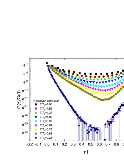
The correlators of and H-dibaryon are presented in Fig. 1 and Fig. 2, respectively. For the correlators of and H-dibaryon, we find similar behavior which was displayed in Fig. 1 in Ref. Aarts:2015mma for . For the correlator of on large and relatively small lattice, especially lattice, some correlator data points are negative, and these points are not displayed on the plot, because the vertical axis is rescaled logarithmically. At some points, the error bar looks strange, it is because at these points, the errors are the magnitude of the correlator value, and the vertical axis is rescaled. For the plot of H-dibaryon correlator, the same observation can be observed.
We use the extrapolation method to extract the ground state masses for , , , , and H-dibaryon. We first fit equation (5) to correlator by suppressing different early time slices to get a series of mass values. We present the results of nucleon and H-dibaryon on lattice in Fig. 3. After we get a series of mass values with different early time slices suppressed, we extrapolate the mass values linearly with the scenario described in the last paragraph in Sec. II. We present the results of linear extrapolation for nucleon and H-dibaryon on lattice in Fig. 4. In the extrapolation procedure, we use one portion of the data presented in Fig. 3.
The results are listed in table 3. We can find that the masses decrease when temperature increases. We compare our results of and below with those in Refs. Aarts:2015mma ; Aarts:2018glk . The results are consistent within errors.
We also calculate the spectral density of the correlation function of , , , and H-dibaryon by using the public computer program Hansen:code .
We present the spectral density with different for , and H-dibaryon at three temperatures in Fig. 5. The upper panel in Fig. 5 for at indicates that too large value may skip peak structure of spectral density. From the upper panel in Fig. 5, we can find that the spectral density distribution obtained by using has just one position where takes locally maximum value. The position is about at . At , the time extent is large enough to extract the ground state energy.
However, even if we do not suppress any early Euclidean time slices in the fitting procedure with equation (5), we cannot get a mass value which is larger than . The largest value of we get by suppressing different number of early time slices is about which is smaller than 0.30. It can be seen clearly from Fig. 3. The mass value of 0.30 is somewhat an arbitrary value between the two peak positions of 0.17 and 0.38 for the spectral density from table 4. So we think taking large may lead to missing some peak structure. On the other hand, spectral density obtained by using in the upper panel of Fig. 5 has a peak position at with small peak value. This peak structure may be due to the lattice artefact.
The middle panel in Fig. 5 for at shows that smaller value can make peak structure of spectral density in small region more pronounced. The lower panel for H-dibaryon at suggests that different value has little effect on the computation of spectral density at high temperature. So, we just present the spectral density results computed with in the following.
The spectral density of , and H-dibaryon are given in Fig. 6, 7 and 8, respectively. The spectral density of and has similar behaviour to that of . From Fig. 6 , 7 and 8, we can find that the spectral density of and has similar behaviour, while of H-dibaryon is slightly different. All the peak positions of are collected in Table 4,5,6,8 and 7.
From Fig. 6, 7 and 8, we can find that at the lowest temperature , the spectral density for , and H-dibaryon has rich peak structure. Despite there are two peaks approximately between and , the spectral density of and in the range of from to are almost the same. The mass values , obtained by extrapolation method are in that range of .
However, at for H-dibaryon is in the neighbour of peak position where the value is not very large. Obtaining at is just by suppressing more early Euclidean time slices. From the upper panel of Fig. 8, more high frequency components of the spectral density should be suppressed in the extrapolation procedure.
When temperature increases, the multi-peak structure of spectral density distribution turns into two-peak structure for and until at high temperature , the spectral density distribution has one peak.
At the intermediate temperatures, the spectral density has a two-peak structure. If we take the smaller values of at peak positions as the ground state energies of corresponding particle, then these mass values obtained by the peak position of are smaller than those mass values obtained in Ref. Aarts:2015mma and Ref. Aarts:2018glk . Mass values of , and presented in Table. 3 are not consistent with the peak positions of corresponding spectral density. This observation shows that the mass values obtained by extrapolation method are affected by the two-peak structure of spectral density.
At high temperature , for the spectral density distribution for , the spectral density exhibits one peak structure, and the peak position shifts towards large value with increasing temperature. In the meantime, we can find the peak broadens and becomes smooth. It means that in the mass spectrum structure of nucleon, there is no function structure contributing to the correlation function. We can find this observation from Fig. 9 for . Similar behaviour can be found for , and . We think the smooth distribution of spectral density implies that there does not exist one-particle state at high temperature.
This is not the case for H-dibaryon. The spectral density distribution for H-dibaryon at is presented in Fig. 10 from which we can find that at , the spectral density distribution still exhibits one peak structure until at , the spectral density distribution broadens and becomes smooth. This observation may imply that at temperature , H-dibaryon still remains as a one-particle state.
V DISCUSSIONS
We have made a simulation in an attempt to determine the masses of the conjectured H-dibaryon with flavor QCD with clover fermion at nine different temperatures. In the meantime, we also calculate the masses of , , and . The results are collected in table 3. The spectral density distribution of those particle’s correlation function are computed to understand the mass spectrum obtained by extrapolation method.
In our simulation, the change of temperature is represented by the change of . is pseudocritical temperature determined via renormalized Polyakov loop and estimated to be Aarts:2014nba ; Aarts:2020vyb .
We have compared two scenarios to obtain the ground state mass as possible as we can. One is to suppress more early Euclidean time slices in the fitting procedure with equation (5). The second method is the extrapolation method. We extrapolate some fitting results which are obtained with different Euclidean time slices suppression to time approaching infinity. The results by the two methods are consistent with each other within errors. We just present the results by the extrapolation method in table 3. In fact, among the series of mass values obtained by different early time suppression, it is difficult to choose which mass value is the proper one. However, the extrapolation method can alleviate this difficulty to some extent.
The analysis of spectral density can provide insights on mass spectrum. However, in our simulation, we can find that the mass values obtained by extrapolation method are not consistent with the peak position of spectral density in some situations, especially at high temperature. Under such situations, we think the results of extrapolation method are more reliable. We can take the peak positions for nucleon in Table 4 as an example to give an explanation. The smaller values of peak position are increasing with temperature. However, with increasing temperature, the mass values of particle concerned are supposed to decrease.
At the lowest temperature , the spectral density distribution has rich peak structure. The mass spectrum of particles approximately reflects the peak position of spectral density distribution.
At the intermediate temperatures, the spectral density distribution exhibits a two-peak structure. The peak structure at the smaller becomes smooth gradually when increases. Considering the quark mass which corresponds to , if we take the smaller at the peak position as the ground state energy, the mass value is too small. So we think the mass values obtained by using extrapolation method are affected by the two states.
At high temperature, despite we get the mass values for , , and which are presented in table 3 by extrapolation method, the spectral density distribution appears to become smooth which implies there does not exist one state.
H-dibaryon is a multi-baryon state. From the spectral density distribution, it is found that at the lowest temperature , the multi-state structure manifests. When temperature increases, the number of peaks decreases until at , the spectral density distribution becomes almost smooth. It means it is likely that H-dibaryon survives beyond until it melts down at . Considering that H-dibaryon is a multi-baryon state, this conclusion awaits further investigation.
It is appropriate to consider the lowest temperature ensembles to be the zero temperature ones since Aarts:2020vyb . Using the mass values of H-dibaryon and in Table 3 at , an estimation of can be made. which is converted into physical unit to be . Ref. Beane:2006mx ; NPLQCD:2012mex ; Inoue:2010es ; Inoue:2011ai ; Francis:2018qch ; Green:2021qol showed the presence of a binding state of H-dibaryon, despite the disagreement on the binding energy values. Ref. Beane:2006mx ; NPLQCD:2012mex reported a binding energy of at , and at . Ref. Inoue:2010es obtained a binding energy of H-dibaryon for pion mass . Ref. Inoue:2011ai had the similar results. Ref. Francis:2018qch published the binding energy of H-dibaryon for . Ref. Green:2021qol presented an estimation of the binding energy in the continuum limit at the SU(3)-symmetric point with ( for the binding energy versus pion mass, see also, Fig. 5 in Ref. Green:2021qol ).
In our simulation, the correlators of proton, and H-dibaryon at have negative values, and in the fitting process for H-dibaryon, we drop the negative values. We guess the emergence of negative values of the correlators is due to deterioration of the signal-to-noise ratio.
Our simualtions are at which is far from physical pion mass, so simulations with lower pion mass are expected to give us more information about the properties of H-dibaryon.
Acknowledgements.
We thank Gert Aarts, Simon Hands, Chris Allton, and Jonas Glesaaen for valuable helps, and thank Chris Allton for the discussion about the extrapolation method. We modify the adapted version of OpenQCD code openqcd to carry out this simulation and we use the computer program Hansen:code to calculate the spectral density of correlation function. The adaptation of OpenQCD code is publicly available fastsum1 . The simulations are carried out on Generation2 (Gen2) FASTSUM ensembles Aarts:2020vyb of which the ensembles at the lowest temperature are provided by the HadSpec collaboration Edwards:2008ja ; HadronSpectrum:2008xlg . This work is supported by the National Natural Science Foundation of China (NSFC) under Grant No. 11347029. This work is done at the high performance computing platform of Jiangsu University.References
- (1) R. L. Jaffe, Phys. Rev. Lett. 38, 195-198 (1977) [erratum: Phys. Rev. Lett. 38, 617(E) (1977)]
- (2) G. R. Farrar, arXiv:1708.08951 [hep-ph].
- (3) S. Aoki, S. Y. Bahk, K. S. Chung, S. H. Chung, H. Funahashi, C. H. Hahn, T. Hara, S. Hirata, K. Hoshino and M. Ieiri, et al. Prog. Theor. Phys. 85, 1287-1298 (1991).
- (4) J. K. Ahn et al. [KEK-PS E224], Phys. Lett. B 444, 267-272 (1998).
- (5) H. Takahashi, J. K. Ahn, H. Akikawa, S. Aoki, K. Arai, S. Y. Bahk, K. M. Baik, B. Bassalleck, J. H. Chung and M. S. Chung, et al. Phys. Rev. Lett. 87, 212502 (2001).
- (6) C. J. Yoon, H. Akikawa, K. Aoki, Y. Fukao, H. Funahashi, M. Hayata, K. Imai, K. Miwa, H. Okada and N. Saito, et al. Phys. Rev. C 75, 022201(R) (2007).
- (7) S. Aoki et al. [KEK E176], Nucl. Phys. A 828, 191-232 (2009).
- (8) K. Nakazawa [KEK-E176 and J-PARC-E07], Nucl. Phys. A 835, 207-214 (2010).
- (9) B. H. Kim et al. [Belle], Phys. Rev. Lett. 110, no.22, 222002 (2013).
- (10) J. P. Lees et al. [BaBar], Phys. Rev. Lett. 122, no.7, 072002 (2019).
- (11) H. Ekawa, K. Agari, J. K. Ahn, T. Akaishi, Y. Akazawa, S. Ashikaga, B. Bassalleck, S. Bleser, Y. Endo and Y. Fujikawa, et al. PTEP 2019, no.2, 021D02 (2019).
- (12) Y. Iwasaki, T. Yoshie and Y. Tsuboi, Phys. Rev. Lett. 60, 1371-1374 (1988).
- (13) Z. H. Luo, M. Loan and Y. Liu, Phys. Rev. D 84, 034502 (2011).
- (14) Z. H. Luo, M. Loan and X. Q. Luo, Mod. Phys. Lett. A 22, 591-597 (2007).
- (15) P. B. Mackenzie and H. B. Thacker, Phys. Rev. Lett. 55, 2539 (1985).
- (16) A. Pochinsky, J. W. Negele and B. Scarlet, Nucl. Phys. B Proc. Suppl. 73, 255-257 (1999).
- (17) I. Wetzorke, F. Karsch and E. Laermann, Nucl. Phys. B Proc. Suppl. 83, 218-220 (2000).
- (18) I. Wetzorke and F. Karsch, Nucl. Phys. B Proc. Suppl. 119, 278-280 (2003).
- (19) S. R. Beane, W. Detmold, H.-W. Lin, T. C. Luu, K. Orginos, M. J. Savage, A. Torok and A. Walker-Loud [NPLQCD], Phys. Rev. D 81, 054505 (2010).
- (20) S. R. Beane et al. [NPLQCD], Phys. Rev. Lett. 106, 162001 (2011).
- (21) S. R. Beane, E. Chang, W. Detmold, B. Joo, H. W. Lin, T. C. Luu, K. Orginos, A. Parreno, M. J. Savage and A. Torok, et al. Mod. Phys. Lett. A 26, 2587-2595 (2011).
- (22) S. R. Beane et al. [NPLQCD], Phys. Rev. D 85, 054511 (2012).
- (23) S. R. Beane et al. [NPLQCD], Phys. Rev. D 87, no.3, 034506 (2013).
- (24) T. Inoue et al. [HAL QCD], Prog. Theor. Phys. 124, 591-603 (2010).
- (25) T. Inoue, N. Ishii, S. Aoki, T. Doi, T. Hatsuda, Y. Ikeda, K. Murano, H. Nemura, and K. Sasaki [HAL QCD], Phys. Rev. Lett. 106, 162002 (2011).
- (26) T. Inoue et al. [HAL QCD], Nucl. Phys. A 881, 28-43 (2012).
- (27) K. Sasaki et al. [HAL QCD], Nucl. Phys. A 998, 121737 (2020).
- (28) K. Sasaki, S. Aoki, T. Doi, S. Gongyo, T. Hatsuda, Y. Ikeda, T. Inoue, T. Iritani, N. Ishii and T. Miyamoto, et al. PoS LATTICE2015, 088 (2016).
- (29) K. Sasaki et al. [HAL QCD], EPJ Web Conf. 175, 05010 (2018).
- (30) A. Francis, J. R. Green, P. M. Junnarkar, C. Miao, T. D. Rae and H. Wittig, Phys. Rev. D 99, no.7, 074505 (2019).
- (31) J. R. Green, A. D. Hanlon, P. M. Junnarkar and H. Wittig, Phys. Rev. Lett. 127, no.24, 242003 (2021).
- (32) S. R. Beane, P. F. Bedaque, A. Parreno and M. J. Savage, Phys. Lett. B 585, 106-114 (2004).
- (33) S. R. Beane, P. F. Bedaque, K. Orginos and M. J. Savage, Phys. Rev. Lett. 97, 012001 (2006).
- (34) M. Luscher, Commun. Math. Phys. 105, 153-188 (1986).
- (35) M. Luscher, Nucl. Phys. B 354, 531-578 (1991).
- (36) P. M. Junnarkar and N. Mathur, Phys. Rev. D 106, no.5, 054511 (2022).
- (37) N. Mathur, M. Padmanath and D. Chakraborty, Phys. Rev. Lett. 130, no.11, 111901 (2023).
- (38) G. Aarts, S. Kim, M. P. Lombardo, M. B. Oktay, S. M. Ryan, D. K. Sinclair and J. I. Skullerud, Phys. Rev. Lett. 106, 061602 (2011).
- (39) G. Aarts, C. Allton, S. Kim, M. P. Lombardo, M. B. Oktay, S. M. Ryan, D. K. Sinclair and J. I. Skullerud, JHEP 11, 103 (2011).
- (40) G. Aarts, C. Allton, S. Kim, M. P. Lombardo, S. M. Ryan and J. I. Skullerud, JHEP 12, 064 (2013).
- (41) G. Aarts, C. Allton, T. Harris, S. Kim, M. P. Lombardo, S. M. Ryan and J. I. Skullerud, JHEP 07, 097 (2014).
- (42) A. Kelly, A. Rothkopf and J. I. Skullerud, Phys. Rev. D 97, no.11, 114509 (2018).
- (43) G. Aarts, C. Allton, J. Glesaaen, S. Hands, B. Jäger, S. Kim, M. P. Lombardo, A. A. Nikolaev, S. M. Ryan and J. I. Skullerud, et al. Phys. Rev. D 105, no.3, 034504 (2022).
- (44) F. Karsch and E. Laermann, Thermodynamics and in medium hadron properties from lattice QCD, Edited by Hwa, R.C. (ed.) et al.: Quark gluon plasma (World Scientific, Singapore, 2004) p. 1-59.
- (45) G. Aarts, C. Allton, D. De Boni and B. Jäger, Phys. Rev. D 99, no.7, 074503 (2019).
- (46) C. E. Detar and J. B. Kogut, Phys. Rev. Lett. 59 (1987) 399; Phys. Rev. D 36 (1987) 2828.
- (47) I. Pushkina et al. [QCD-TARO Collaboration], Phys. Lett. B 609 (2005) 265.
- (48) S. Datta, S. Gupta, M. Padmanath, J. Maiti and N. Mathur, JHEP 1302 (2013) 145.
- (49) G. Aarts, C. Allton, S. Hands, B. Jäger, C. Praki and J. I. Skullerud, Phys. Rev. D 92 (2015) no.1, 014503.
- (50) M. Hansen, A. Lupo and N. Tantalo, Phys. Rev. D 99, no.9, 094508 (2019).
- (51) J. Donoghue, E. Golowich, and B. R. Holstein, Phys. Rev. D 34,3434, (1986).
- (52) E. Golowich and T. Sotirelis, Phys. Rev. D 46,354, (1992).
- (53) I. Wetzorke, https://pub.uni-bielefeld.de/record/2394939.
- (54) D. B. Leinweber, W. Melnitchouk, D. G. Richards, A. G. Williams and J. M. Zanotti, Lect. Notes Phys. 663, 71-112 (2005).
- (55) I. Montvay and G. Münster, “Quantum fields on a lattice,” Cambridge, UK: Univ. Pr. (1994) 491 p. (Cambridge monographs on mathematical physics).
- (56) C. Gattringer and C. B. Lang, “Quantum chromodynamics on the lattice,” Lect. Notes Phys. 788 (2010) 1.
- (57) M. Asakawa, T. Hatsuda and Y. Nakahara, Prog. Part. Nucl. Phys. 46, 459-508 (2001).
- (58) Y. Burnier and A. Rothkopf, Phys. Rev. Lett. 111, 182003 (2013).
- (59) G. Aarts, C. Allton, J. Foley, S. Hands and S. Kim, Phys. Rev. Lett. 99, 022002 (2007).
- (60) B. B. Brandt, A. Francis, H. B. Meyer and D. Robaina, Phys. Rev. D 92, no.9, 094510 (2015).
- (61) B. B. Brandt, A. Francis, B. Jäger and H. B. Meyer, Phys. Rev. D 93, no.5, 054510 (2016).
- (62) A. Lupo, L. Del Debbio, M. Panero and N. Tantalo, PoS LATTICE2023 (2024), 004.
- (63) A. Barone, S. Hashimoto, A. Jüttner, T. Kaneko and R. Kellermann, [arXiv:2312.17401 [hep-lat]].
- (64) A. Rothkopf, EPJ Web Conf. 274, 01004 (2022).
- (65) H. Meyer, PoS INPC2016, 364 (2017).
- (66) R. G. Edwards, B. Joo and H. W. Lin, Phys. Rev. D 78, 054501 (2008).
- (67) H. W. Lin et al. [Hadron Spectrum], Phys. Rev. D 79, 034502 (2009).
- (68) M. Luscher, JHEP 12, 011 (2007).
- (69) M. Luscher, JHEP 07, 081 (2007).
- (70) S. Gusken, U. Low, K. H. Mutter, R. Sommer, A. Patel and K. Schilling, Phys. Lett. B 227, 266-269 (1989).
- (71) C. Morningstar and M. J. Peardon, Phys. Rev. D 69, 054501 (2004).
- (72) https://github.com/mrlhansen/rmsd.
- (73) G. Aarts, C. Allton, A. Amato, P. Giudice, S. Hands and J. I. Skullerud, JHEP 02, 186 (2015).
- (74) OpenQCD, luscher.web.cern.ch/luscher/openQCD/.
- (75) FASTSUM Collaboration, http://fastsum.gitlab.io/.