Mass-shifting phenomenon of truncated multivariate normal priors
Abstract
We show that lower-dimensional marginal densities of dependent zero-mean normal distributions truncated to the positive orthant exhibit a mass-shifting phenomenon. Despite the truncated multivariate normal density having a mode at the origin, the marginal density assigns increasingly small mass near the origin as the dimension increases. The phenomenon accentuates with stronger correlation between the random variables. A precise quantification characterizing the role of the dimension as well as the dependence is provided. This surprising behavior has serious implications towards Bayesian constrained estimation and inference, where the prior, in addition to having a full support, is required to assign a substantial probability near the origin to capture flat parts of the true function of interest. Without further modification, we show that truncated normal priors are not suitable for modeling flat regions and propose a novel alternative strategy based on shrinking the coordinates using a multiplicative scale parameter. The proposed shrinkage prior is empirically shown to guard against the mass shifting phenomenon while retaining computational efficiency.
1 Introduction
Let denote the density of a distribution truncated to the non-negative orthant in ,
| (1.1) |
The density is clearly unimodal with its mode at the origin. However, for certain classes of non-diagonal , we surprisingly observe that the lower-dimensional marginal distributions increasingly shift mass away from the origin as increases. This observation is quantified in Theorem 2, where we provide non-asymptotic estimates for marginal probabilities of events of the form , for . En-route to the proof, we derive a novel Gaussian comparison inequality in Lemma 1. An immediate implication of this mass-shifting phenomenon is that corner regions of the support , where a subset of the coordinates take values close to zero, increasingly become low-probability regions under as dimension increases. From a statistical perspective, this helps explain a paradoxical behavior in Bayesian constrained regression empirically observed in Neelon and Dunson, (2004) and Curtis and Ghosh, (2011), where truncated normal priors led to biased posterior inference when the underlying function had flat regions.
A common approach towards Bayesian constrained regression expands the function in a flexible basis which facilitates representation of the functional constraints in terms of simple constraints on the coefficient space, and then specifies a prior distribution on the coefficients obeying the said constraints. In this context, the multivariate normal distribution subject to linear constraints arises as a natural conjugate prior in Gaussian models and beyond. Various basis, such as Bernstein polynomials (Curtis and Ghosh,, 2011), regression splines (Cai and Dunson,, 2007; Meyer et al.,, 2011), penalized spines (Brezger and Steiner,, 2008), cumulative distribution functions (Bornkamp and Ickstadt,, 2009), restricted splines (Shively et al.,, 2011), and compactly supported basis (Maatouk and Bay,, 2017) have been employed in the literature. For numerical illustrations in this article, we shall use the formulation of Maatouk and Bay, (2017) where various restrictions such as boundedness, monotonicity, convexity, etc were equivalently translated into non-negativity constraints on the coefficients under an appropriate basis expansion. They used a truncated normal prior as in (1.1) on the coefficients, with induced from a parent Gaussian process on the regression function; see Appendix A for more details.
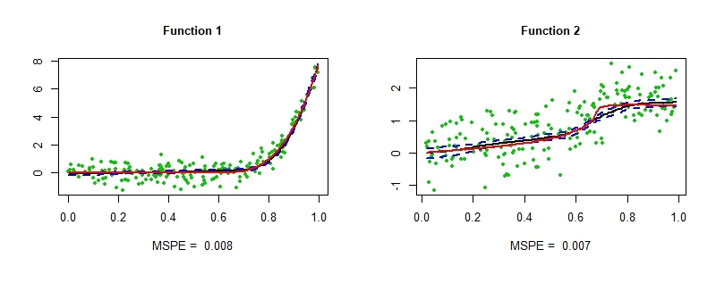
To motivate our theoretical investigations, the two panels in Figure 1 depict the estimation of two different monotone smooth functions on based on 100 samples using the basis of Maatouk and Bay, (2017) and a joint prior as in (1.1) on the dimensional basis coefficients. The same prior scale matrix was employed across the two settings; the specifics are deferred to Section 3 and Appendix A. Observe that the function in the left panel is strictly monotone, while the one on the right panel is relatively flat over a region. While the point estimate (posterior mean) as well as the credible intervals look reasonable for the function in the left panel, the situation is significantly worse for the function in the right panel. The posterior mean incurs a large bias, and the pointwise 95 credible intervals fail to capture the true function for a substantial part of the input domain, suggesting that the entire posterior distribution is biased away from the truth. This behavior is perplexing; we are fitting a well-specified model with a prior that has full support111the prior probability assigned to arbitrarily small Kullback–Leibler neighborhoods of any point is positive. on the parameter space, which under mild conditions implies good first-order asymptotic properties (Ghosal et al.,, 2000) such as posterior consistency. However, the finite sample behavior of the posterior under the second scenario clearly suggests otherwise.
Functions with flat regions as in the right panel of Figure 1 routinely appear in many applications; for example, dose-response curves are assumed to be non-decreasing with the possibility that the dose-response relationship is flat over certain regions (Neelon and Dunson,, 2004). A similar biased behavior of the posterior for such functions under truncated normal priors was observed by Neelon and Dunson, (2004) while using a piecewise linear model, and also by Curtis and Ghosh, (2011) under a Bernstein polynomial basis. However, a clear explanation behind such behavior as well as the extent to which it is prevalent has been missing in the literature, and the mass-shifting phenomenon alluded before offers a clarification. Under the basis of Maatouk and Bay, (2017), a subset of the basis coefficients are required to shrink close to zero to accurately approximate functions with such flat regions. However, the truncated normal posterior pushes mass away from such corner regions, leading to the bias. Importantly, our theory also suggests that the problem would not disappear and would rather get accentuated in the large sample scenario if one follows standard practice of scaling up the number of basis functions with increasing sample size, since the mass-shifting gets more pronounced with increasing dimension. To illustrate this point, Figure 2 shows the estimation of the same function in the right panel of Figure 1, now based on 500 samples and and basis functions in the left and right panel respectively. Increasing the number of basis functions indeed results in a noticeable increase in the bias as clearly seen from the insets which zoom into two disjoint regions of the covariate domain. A similar story holds for the basis of Neelon and Dunson, (2004) and Curtis and Ghosh, (2011).


Neelon and Dunson, (2004) and Curtis and Ghosh, (2011) both used point-mass mixture priors as remedy, which is a natural choice under a non-decreasing constraint. However, their introduction becomes somewhat cumbersome under the non-negativity constraint in (1.1). As a simple remedy, we suggest introducing a multiplicative scale parameter for each coordinate a priori and further equipping it with a prior mixing distribution which has positive density at the origin and heavy tails; a default candidate is the half-Cauchy density (Carvalho et al.,, 2010). The resulting prior shrinks much more aggressively towards the origin, and we empirically illustrate its superior performance over the truncated normal prior. This empirical exercise provides further support to our argument.
2 Mass-shifting phenomenon of truncated normal distributions
2.1 Marginal densities of truncated normal distributions
Our main focus is on studying the properties of marginal densities of truncated normal distributions described in equation (1.1) and quantifying how they behave with increasing dimensions. We begin by introducing some notation. We use to denote the -dimensional normal distribution with mean and positive definite covariance matrix ; also let denote its density evaluated at . We reserve the notation to denote the compound-symmetry correlation matrix with diagonal elements equal to and off-diagonal elements equal to ,
| (2.1) |
with the vector of ones in and the identity matrix.
For a subset with positive Lebesgue measure, let denote a distribution truncated onto , with density
| (2.2) |
where for is the constant of integration and the indicator function of the set . We throughout assume to be the positive orthant of as in equation (1.1), namely, ; a general defined by linear inequality constraints can be reduced to rectangular constraints using a linear transformation - see, for example, § 2 of Botev, (2017). The dimension will be typically evident from the context.
Our investigations were originally motivated by the following observation. Consider for . Then, the marginal distribution of has density proportional to on , where denotes the cumulative distribution function. This distribution is readily recognized as a skew normal density (Azzalini and Valle,, 1996) truncated to . Interestingly, the marginal of has a strictly positive mode, while the joint distribution of had its mode at . Cartinhour, (1990) noted that the truncated normal family is not closed under marginalization for non-diagonal , and derived a general formula for the univariate marginal as the product of a univariate normal density with a skewing factor. In Proposition 1 below, we generalize Cartinhour’s result for any lower-dimensional marginal density. We write the scale matrix in block form as .
Proposition 1.
Suppose . The marginal density of is
where with , and the symbol is to be interpreted elementwise. Here, the constant for .
When , Proposition 1 implies
| (2.3) |
Let denote the set of covariance matrices whose correlation coefficients are all non-negative. The map is decreasing and when , is increasing, on . Thus, if , is unimodal with a strictly positive mode.
As another special case, suppose for some and let . We then have,
with , where is a positive constant. This density can be recognized as a multivariate skew-normal distribution (Azzalini and Valle,, 1996) truncated to the non-negative orthant.
2.2 Mass-shifting phenomenon of marginal densities
While the results in the previous section imply that the marginal distributions shift mass away from the origin, they do not precisely characterize the severity of its prevalence. In this section, we show that under appropriate conditions, the univariate marginals assign increasingly smaller mass to a fixed neighborhood of the origin with increasing dimension. In other words, the skewing factor noted by Cartinhour begins to dominate when the ambient dimension is large. In addition to the dimension, we also quantify the amount of dependence in contributing to this mass-shifting. To the best of our knowledge, this has not been observed or quantified in the literature.
We state our results for , where for , denotes the space of -banded nonnegative correlation matrices,
| (2.4) |
While our main theorem below can be proved for other dependence structures, the banded structure naturally arises in statistical applications as discussed in the next section.
Given , define and to be the maximum and minimum correlation values within the band. For with , let . With these definitions, we are ready to state our main theorem.
Theorem 2.
Let be such that , where
Then, there exists a constant such that whenever , we have for any ,
where is a positive rational function of , and is a constant free of .
In particular, if we consider a sequence of -banded correlation matrices with as , then under the conditions of Theorem 2, for any fixed . Theorem 2, being non-asymptotic in nature, additionally characterizes the rate of decay of . To contrast the conclusion of Theorem 2 with two closely related cases, consider first the case when . For any , the marginal distribution of is always , and hence does not depend on . Similarly, if with a diagonal correlation matrix, then for any , the marginal distribution of is truncated to and again does not depend on . In particular, in both these cases, for small. However, when a combination of dependence and truncation is present, an additional penalty is incurred.

For the conclusion of Theorem 2 to hold, our current proof technique requires to lie in the region , which is pictorially represented by the black shaded region in Figure 3. As a special case, if all the non-zero correlations are the same, i.e., , then the condition simplifies to . More generally, if we write for some , then the condition reduces to .
Remark 1.
For any fixed , the marginal density of evaluated at the origin, . Theorem 2 thus implies in particular that . Also, for any fixed , if we denote , it is immediate that , and hence , meaning the probability of a corner region is vanishingly small for large .
We now empirically illustrate the conclusion of the theorem by presenting the univariate marginal density for different values of the dimension and the bandwidth . The density calculations were performed using the R package tmvtnorm, which is based on the numerical approximation algorithm proposed in Cartinhour, (1990) and subsequent refinements in Genz, (1992, 1993); Genz and Bretz, (2009).


The left panel of Figure 4 shows that for fixed at a moderately large value, the probability assigned to a small neighborhood of the origin decreases with increasing . Also, the mode of the marginal density increasingly shifts away from zero. A similar effect is seen for a fixed and increasing in the middle panel and also for an increasing pair in the right panel, although the mass-shifting effect is somewhat weakened compared to the left panel. This behavior perfectly aligns with the main message of the theorem that the interplay between the truncation and the dependence brings forth the mass-shifting phenomenon.
The proof of Theorem 2 is non-trivial; we provide the overall chain of arguments in the next subsection, deferring the proof of several auxiliary results to the supplemental document. The marginal probability of is a ratio of the probabilities of two rectangular regions under a distribution, with the denominator appearing due to the truncation. While there is a rich literature on estimating tail probabilities under correlated multivariate normals using multivariate extensions of the Mill’s ratio (Savage,, 1962; Ruben,, 1964; Sidák,, 1968; Steck,, 1979; Hashorva and Hüsler,, 2003; Lu,, 2016), the existing bounds are more suited for numerical evaluation (Cartinhour,, 1990; Genz,, 1992; Genz and Bretz,, 2009) and pose analytic difficulties due to their complicated forms. Moreover, the current bounds lose their accuracy when the region boundary is close to the origin (Gasull and Utzet,, 2014), which is precisely our object of interest. Our argument instead relies on novel usage of Gaussian comparison inequalities such as the Slepian’s inequality; see Li and Shao, (2001); Vershynin, 2018a for book-level treatments. We additionally derive a generalization of Slepian’s inequality in Lemma 1, which might be of independent interest. As an important reduction step, we introduce a blocking idea to carefully approximate the banded scale matrix by a block tridiagonal matrix to simplify the analysis.
2.3 Proof of Theorem 2
By definition,
| (2.5) |
where . We now proceed to separately bound the numerator and denominator in the above display.
We first consider the denominator in equation (2.5), and use Slepian’s lemma to bound it from below. It follows from Slepian’s inequality, see comment after Lemma 3 in the supplemental document, that if are centered -dimensional Gaussian random variables with for all , and for all , then
| (2.6) |

The Slepian’s inequality is a prominent example of a Gaussian comparison inequality originally developed to bound the supremum of Gaussian processes. To apply Slepian’s inequality to the present context, we construct another -dimensional centered Gaussian random vector such that (i) , and , and (ii) the sub-vectors , and are mutually independent. The correlation matrix of clearly satisfies for all by construction. Figure 5 pictorially depicts this block approximation in an example with and . Applying Slepian’s inequality, we then have,
| (2.7) |
Next, we consider the numerator in equation (2.5). We have,
| (2.8) |
The last equality crucially uses and are independent, which is a consequence of being -banded. Taking the ratio of equations (2.3) and (2.3), the term cancels so that
| (2.9) |
To bound the terms and in the denominator of , we resort to another round of Slepian’s inequality. Let , where recall that is the minimum non-zero correlation in . Also, recall from equation (2.1) that denotes the compound-symmetry correlation matrix with all correlations equal to . By construction, for any , . Thus, applying Slepian’s inequality as in equation (2.6), {equs}P(Z_[1 : K]≥0) P(Z_[K+1 : 2K]≥0) ≥{P(Z” ≥0)}^2.
The numerator of equation (2.9) cannot be directly tackled by Slepian’s inequality, and we prove the following comparison inequality in the supplemental document.
Lemma 1.
(Generalized Slepian’s inequality) Let be centered -dimensional Gaussian vectors with for all and for all . Then for any and , we have {equs}P(ℓ_1 ≤X_1≤u_1 , X_2 ≥u_2, …, X_d ≥u_d) ≤P(ℓ_1 ≤Y_1 ≤u_1, Y_2 ≥u_2, …, Y_d ≥u_d).
Define a random variable and use Lemma 1 to conclude that .
Substituting these bounds in equation (2.9), we obtain
| (2.10) |
The primary reduction achieved by bounding by is that we only need to estimate Gaussian probabilities under a compound-symmetry covariance structure. We prove the following inequalities in the supplemental document that provide these estimates.
Lemma 2.
Let with . Fix . Define . Then,
for any . Also,
A key aspect of the compound-symmetry structure that we exploit is for with , we can represent , where ’s are independent variables.
Using Lemma 2, we can bound, for any ,
| (2.11) |
with . Since , we have , or equivalently, . Thus, we can always find such that . Fix such an , and substitute in equation (2.3). The proof is now completed by choosing large enough so that for any , the second term in the last line of (2.3) is smaller than the first; this is possible since the second term decreases exponentially while the first does so polynomially in .
3 Connections with Bayesian constrained inference
In this section, we connect the theoretical findings in the previous section to posterior inference in Bayesian constrained regression models. We work under the setup of a usual Gaussian regression model,
| (3.1) |
where we assume for simplicity. We are interested in the situation when the regression function is constrained to lie in some space which is a subset of the space of all continuous functions on , determined by linear restrictions on and possibly its higher-order derivatives. Common examples include bounded, monotone, convex, and concave functions.
As discussed in the introduction, a general approach is to expand in some basis as so that the restrictions on can be posed as linear restrictions on the vector of basis coefficients , with the parameter space for of the form . For example, when corresponds to monotone increasing functions, the set is of the form under the Bernstein polynomial basis (Curtis and Ghosh,, 2011) and under the integrated triangular basis of Maatouk and Bay, (2017). For sake of concreteness, we shall henceforth work with . Under such a basis representation, the model (3.1) can be expressed as
| (3.2) |
where and is an basis matrix.
The truncated normal prior is conjugate, with the posterior , with
To motivate their prior choice, Maatouk and Bay, (2017) begin with an unconstrained mean-zero Gaussian process prior on , , with covariance kernel . Since their basis coefficients correspond to evaluation of the function and its derivatives at the grid points; see Appendix A for details; this induces a multivariate zero-mean Gaussian prior on provided the covariance kernel of the parent Gaussian process is sufficiently smooth. Having obtained this unconstrained Gaussian prior on , Maatouk and Bay, (2017) multiply it with the indicator function of the truncation region to obtain the truncated normal prior.
We are now in a position to connect the posterior bias in Figures 1 and 2 to the mass-shifting phenomenon characterized in the previous section. Since the posterior , a draw from the posterior can be represented as
Consider an extreme scenario when the true function is entirely flat. In this case, the optimal parameter value and under mild assumptions, is concentrated near the origin with high probability under the true data distribution; see §E of the supplementary material. The mass shifting phenomenon pushes away from the origin, resulting in the bias. On the other hand, when the true function is strictly monotone as in the left panel of Figure 1, all the entries of are bounded away from zero, which masks the effect of the shift in .
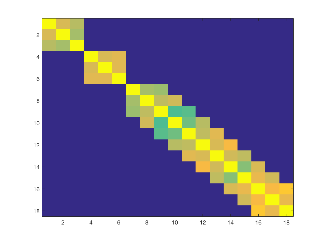
In strict technical terms, our theory is not directly applicable to since the scale matrix is a dense matrix in general. However, we show below that is approximately banded under mild conditions. Figure 6 shows image plots of for three choices of using the basis of Maatouk and Bay, (2017) and sample size . In all cases, is seen to have a near-banded structure.


We make this empirical observation concrete below. We first state the assumptions on the basis matrix and prior covariance matrix that allows the construction of a strictly banded matrix approximation.
Assumption 1.
We assume the basis matrix is such that the matrix is -banded for some ; also there exists constants such that
One example of a basis satisfying Assumption 1 is a B-Spline of fixed order denoted as with over quasi-uniform knot points of number ; see, for example, Yoo et al., (2016).
Regarding the prior covariance matrix, we first define a uniform class of symmetric positive definite well-conditioned matrices (Bickel et al., 2008b, ) as
| (3.3) | ||||
Assumption 2.
We assume the prior covariance matrix defined in (3.3).
Assumption 2 ensures the covariance matrix is “approximately bandable”, which is common in covariance matrix estimation with thresholding techniques (Bickel et al., 2008a, ; Bickel et al., 2008b, ).
Given above Assumptions, we are now ready to give the approximation result of posterior scale matrix to a banded symmetric positive definite matrix.
Proposition 3.
Proposition 3 states under mild conditions we can always construct a banded positive definite matrix that approximates in operator norm. Applying the result in Theorem 2 to a truncated normal distribution with the banded approximation of the posterior scale matrix, the marginal density would present a mass-shifting behavior. If we control the band width such that the approximation is close enough to the posterior scale matrix, the marginal posterior distribution would be expected to behave similarly and shift its probability mass away from the origin and the probability mass over the “corner region” will decrease to zero as the dimension goes to infinity. This helps explain the bias occurred in the posterior mean over the flat area shown in the Figure 1.
4 A de-biasing remedy based on a shrinkage prior
As concluded in previous sections, we view the mass-shifting behavior of the posterior marginals causing the bias in posterior estimation for flat functions. In this section, we will provide empirical evidences that a simple modification to the truncated normal prior can alleviate the issues related to such mass-shifting phenomenon. Among remedies proposed in the literature, Curtis and Ghosh, (2011) proposed independent shrinkage priors on the parameter vector given by a mixture of a point-mass at zero and a univariate normal distribution truncated to the positive real line as an alternative to the truncated normal prior,
Similar mixture priors were also previously used by Neelon and Dunson, (2004) and Dunson, (2005). The mass at zero allows positive prior probability to functions having exactly flat regions. Although possible in principle, introduction of such point-masses while retaining the dependence structure between the coefficients becomes somewhat cumbersome in addition to being computationally burdensome. With such motivation and the additional consideration that in most real scenarios a function is approximately flat in certain regions, we propose a shrinkage procedure as a remedy to replace the coefficients by , where
| (4.1) |
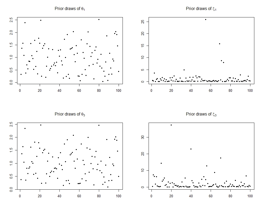
The parameter provides global shrinkage towards the origin while the s provide coefficient-specific deviation. We consider default (Carvalho et al.,, 2010) half-Cauchy priors on and the s independently. The distribution has a density proportional to . We continue to use a dependent truncated normal prior which in turn induces dependence among the s. Our prior on can thus be considered as a dependent extension of the global-local shrinkage priors (Carvalho et al.,, 2010) widely used in the high-dimensional regression context. Figure 9 in §D.1 of the supplementary material shows prior draws for the first and third components of both and , based on which the marginal distribution of the s is clearly seen to place more mass near the origin while retaining heavy tails.
We provide an illustration of the proposed shrinkage procedure in the context of estimating monotone functions as described in (A.1). The procedure can be readily adapted to include various other constraints. Replacing by in (M) in (A.1), we can write (3.1) in vector notation as
| (4.2) |
Here, is an basis matrix with row where for and the basis functions are as in (A.1). Also, , and .
The model is parametrized by , , , and . We place a flat prior on . We place a truncated normal prior on independently of , and with
and is the stationary Matérn kernel with smoothness parameter and length-scale parameter . To complete the prior specification, we place improper prior on and compactly supported priors and on and . We develop a data-augmentation Gibbs sampler which combined with the embedding technique of Ray et al., (2019) results in an efficient MCMC algorithm to sample from the joint posterior of ; the details are deferred to §D.2 of the supplementary material.
We conduct a small-scale simulation study to illustrate the efficacy of the proposed shrinkage procedure. We consider model (3.1) with true and two different choices of the true , namely,
for . The function , which is non-decreasing and flat between and , was used as the motivating example in the introduction. The function is also approximately flat between and , although it is not strictly non-decreasing in this region, which allows us to evaluate the performance under slight model misspecification.
To showcase the improvement due to the shrinkage, we consider a cascading sequence of priors beginning with only a truncated normal prior and gradually adding more structure to eventually arrive at the proposed shrinkage prior. Specifically, the variants considered are
No shrinkage and fixed hyperparameters: Here, we set and in (4.2), and also fix and , so that we have a truncated normal prior on the coefficients. This was implemented as part of the motivating examples in the introduction. We fix and so that the correlation between the maximum separated points in the covariate domain equals .
No shrinkage with hyperparameter updates: The only difference from the previous case is that and are both assigned priors described previously and updated within the MCMC algorithm.
Global shrinkage: We continue with and place a half-Cauchy prior on the global shrinkage parameter . The hyperparameters and are updated.
Global-local shrinkage: This is the proposed procedure where the s are also assigned half-Cauchy priors and the hyperparameters are updated.
We generate pairs of response and covariates and randomly divide the data into training samples and test samples. For all of the variants above, we set the number of knots . We provide plots of the function fit along with pointwise credible intervals in Figures 7 and 8 respectively, and also report the mean squared prediction error (mspe) at the bottom of the sub-plots. As expected, only using the truncated normal prior leads to a large bias in the flat region. Adding some global structure to the truncated normal prior, for instance, updating the gp hyperparamaters and adding a global shrinkage term improves estimation around the flat region, which however still lacks the flexibility to transition from the flat region to the strictly increasing region. The global-local shrinkage performs the best, both visually and also in terms of mspe.
Additionally, the shrinkage procedure performed at least as good as bsar, a very recent state-of-the-art method, developed by Lenk and Choi, (2017), and implemented in the R package bsamGP. For the out-of-sample prediction performance of bsar, refer to Figure 10 in §D.3 of the supplementary material, based on which it is clear that the performance of global-local shrinkage procedure is comparable with that of bsar. It is important to point out that bsar is also a shrinkage based method that allows for exact zeros in the coefficients in a transformed Gaussian process prior through a spike and slab specification.


5 Discussion
A seemingly natural way to define a prior distribution on a constrained parameter space is to consider the restriction of a standard unrestricted prior to the constrained space. The conjugacy properties of the unrestricted prior typically carry over to the restricted case, facilitating computation. Moreover, reference priors on constrained parameters are typically the unconstrained reference prior multiplied by the indicator of the constrained parameter space (Sun and Berger,, 1998). Despite these various attractive properties, the findings of this article pose a caveat towards routine truncation of priors in moderate to high-dimensional parameter spaces, which might lead to biased inference. This issue gets increasingly severe with increasing dimension due to the concentration of measure phenomenon (Talagrand,, 1995; Boucheron et al.,, 2013), which forces the prior to increasingly concentrate away from statistically relevant portions of the parameter space. A somewhat related issue with certain high-dimensional shrinkage priors has been noted in Bhattacharya et al., (2016). Overall, our results suggest a careful study of the geometry of truncated priors as a useful practice. Understanding the cause of the biased behavior also suggests natural shrinkage procedures that can guard against such unintended consequences. We note that post-processing approaches based on projection (Lin and Dunson,, 2014) and constraint relaxation (Duan et al.,, 2020) do not suffer from this unintended bias. The same is also true for the recently proposed monotone bart (Bayesian Additive Regression Trees) (Chipman et al.,, 2010) method.
It would be interesting to explore the presence of similar issues arising from truncations beyond the constrained regression setting. Possible examples include correlation matrix estimation and simultaneous quantile regression. Priors on correlation matrices are often prescribed in terms of constrained priors on covariance matrices, and truncated normal priors are used to maintain ordering between quantile functions corresponding to different quantiles, and this might leave the door open for unintended bias to creep in.
Appendix
Appendix A Basis representation of Maatouk and Bay, (2017)
As our example which motivates the main results of this paper, we consider the more recent basis sequence of Maatouk and Bay, (2017). Let be equally spaced points on , with spacing . Let,
for , where is the “hat function” on . For any continuous function , the function approximates by linearly interpolating between the function values at the knots , with the quality of the approximation improving with increasing . With no additional smoothness assumption, this suggests a model for as .
The basis and take advantage of higher-order smoothness. If is once or twice continuously differentiable respectively, then by the fundamental theorem of calculus,
Expanding and in the interpolation basis as in the previous paragraph respectively imply the models
| (A.1) |
Under the above, the coefficients have a natural interpretation as evaluations of the function or its derivatives at the grid points. For example, under (M), for , while under (C), for .
Maatouk and Bay, (2017) showed that under the representation (M) in (A.1), is monotone non-decreasing if and only if for all . Similarly, under (C), is convex non-decreasing if and only if for all . The ability to equivalently express various constraints in terms of linear restrictions on the vector is an attractive feature of this basis not necessarily shared by other basis.
In either case, the parameter space for is the non-negative orthant . If were unrestricted, a gp prior on would induce a dependent Gaussian prior on . The approach of Maatouk and Bay, (2017) is to restrict this dependent prior subject to the linear restrictions, resulting in a truncated normal prior.
Supplementary Material
In this supplementary document, we first collect all remaining technical proofs in the first two sections. §D provides additional details on prior illustration, posterior computation, and posterior performance. In §E we formulate the concentration property of the posterior center . Several auxiliary results used in the proofs are listed in §F.
Appendix B Proofs of auxiliary results in the proof of Theorem 2
In this section, we provide proofs of Lemma 1 and Lemma 2 that were used to prove Theorem 2 in the main manuscript. For any -dimensional vector we denote its sub-vector for any . For two vectors and of the same length, let () denote the event () for all . For two random variables and , We write if and are identical in distribution.
B.1 Proof of Lemma 1
For random vectors and , to show , it suffices to show
| (B.1) | |||
We define -dimensional indicator functions and , then it is equivalent to show
| (B.2) |
We now construct non-decreasing approximating functions of with continuous second order derivatives respectively. Let be a non-decreasing twice differentiable function with for , for , and for . Also, choose so that for some universal constant . For , we define . It is clear that approximates for large . In fact, for any , .
Given the above, let for , and , for . Define
It then follows that and provide increasingly better approximations of and as . It thus suffices to show
| (B.3) |
for sufficiently large to be chosen later. We henceforth drop the superscript from and for notation brevity.
We proceed to utilize an interpolation technique commonly used to prove comparison inequalities (see Chapter 7 of Vershynin, 2018b ). We construct a sequence of interpolating random variables based on the independent random variables :
Specifically, we have , , and for any , where . For any twice differentiable function , we have the following identity
| (B.4) |
Applying a multivariate version of Stein’s lemma (Lemma 7.2.7 in Vershynin, 2018b ) to the integrand in (B.4), one obtains
| (B.5) |
To show (B.3), we define the difference . We further decompose as
The second equation follows from (B.4) and the third equation follows from . First we show . Since for all , it suffices to show that for any fixed and for any ,
We consider a generic interpolating random variable by dropping the -subscript; let denote its probability density function. Then we have
To guarantee is non-negative we need the integral over to be non-negative. Based on the definition of and , the integral over can be simplified to
| (B.6) |
Let us denote the inverse of the covariance matrix as
where is a scalar. To check the non-negativity of the last line in (B.1), we now estimate the term
where . Since , we have . We denote as the largest element of . Then, one can choose large enough such that
to guarantee . For example satisfies the above inequality.
Now we show . We have for all . For any , for any fixed , we define {equs}D_2 = E( ∂2f∂xi∂xj(S_t) - ∂2g∂xi∂xj(S_t) ) = E{ (f_1 - g_1)f’_i g’_j Π_k≠1,i,jf_k }. Since , and for all , it follows that and thus . Combining with the non-negativity of completes the proof of Lemma B.1.
B.2 Proof of Lemma 2
For with , we will repeatedly use its equivalent expression
| (B.7) |
where ’s are independent standard normal variables.
Proof of the upper bound. We recall . For any fixed and , we have
| (B.8) | ||||
First, we estimate in (B.8). By applying the equivalent expression of in (B.7), we have
Combining bounds for and , we obtain
for any . We then complete the proof of the upper bound.
Proof of the lower bound. We provide a more general result for the lower bound. We show that for any scalar , we have
| (B.9) |
where recall that denotes a -dimensional vector of ones. By taking leads to the desired lower bound in Lemma 2.
Now we prove the lower bound in (B.9). First,
| (B.10) | ||||
where . Here, holds since for and .
We now proceed to lower bound the right hand side of the last equation in (B.10). To that end, we define , where . Importantly, is non-increasing function of for , and is a convex function of for . For any fixed , since is non-increasing in , we have . We then apply Jensen’s inequality,
The last inequality holds by applying Lemma 4 in Appendix F. To lower bound we apply Lemma 5 in Appendix F. Eventually, we obtain
This completes the proof for the lower bound.
Appendix C Remaining proofs from the main document
C.1 Proof of the Proposition 1
Now we derive the -dimensional marginal density function. We denote and . We partition into appropriate blocks as
We also partition its inverse matrix ,
Then the -dimensional marginal
where
and .
C.2 Proof of Proposition 3
We first introduce some notations that are used in the proof. For a matrix , we denote as its th eigenvalue, and denote and as the minimum and maximum of eigenvalues, respectively. For a matrix , we define its operator norm as . For two quantities , we write when can be bounded from below and above by two finite constants.
We repeatedly apply Newmann series and Lemma 6 in Appendix F to construct the approximation matrix to the posterior scale matrix . Under Assumption 2, we have the prior covariance matrix for some universal constants . Then for any , by choosing , one can find a -banded symmetric and positive definite matrix such that
| (C.1) |
Now we let and . Given (C.1), we have
| (C.2) |
By choosing , simple calculation gives . We now apply Newmann series to construct a polynomial of of degree , defined as , for some integer to be chosen later. Applying Lemma 6 in Appendix F, we have
| (C.3) |
where . Applying Lemma 6 we guarantee is -banded and positive definite. Combining results in (C.2) and (C.3), we have
| (C.4) |
Now we let . Under Assumption 1 we have is -banded with We then define and . Thus, given (C.4), we have
for constants in Assumption 2.
We first consider the case where for some constant , as . For sufficiently large , we obtain
| (C.5) |
for constants satisfying and .
Secondly, we consider the case where as . In this case, dominates in the eigenvalues of . Thus, for sufficiently large , we have
| (C.6) |
Now we apply Lemma 6 one more time to construct the approximation matrix to the inverse of . Again, by taking , we have . Now we define for some positive integer . Also, it follows
| (C.7) |
where . By construction is -banded.
Now we estimate . For large enough in the first case, we can upper bound
The inequality holds since the map is non-increasing in . Combing this with the result in (C.5) and taking leads to the expression of . Based on (C.7), we have . For in the second case, following a similar line of argument, we have with .
We recall the posterior scale matrix . Then we have
where and . The first inequality follows from the triangular inequality and the second inequality follows from the identity for invertible matrices . The last inequality follows from results in (C.1) and (C.3).
For in the first case, and are upper bounded by some constants that are free of given (C.5). Then we obtain
where .
Appendix D Additional details on the numerical studies
D.1 Prior draws
We consider equation (4.1) and the prior specified in section 4. Prior samples on both and of dimension were drawn. Figure 9 shows prior draws for the first and third components of both and .
D.2 Posterior Computations
We now consider model (4.2) and the prior specified in section 4. Then the full conditional distribution of
can be approximated by
where is a large valued constant, and . The above is same as equation (5) of Ray et al., (2019) and thus falls under the framework of their sampling scheme. For more details on the sampling scheme and the approximation, one can refer to Ray et al., (2019).
Note that , can be equivalently given by . Thus the full conditional distribution of can be approximated by:
where plays the same role as , , , and . Thus, can be sampled efficiently using algorithm proposed in Ray et al., (2019).
D.3 Performance of bsar
Consider the simulation set-up specified in section 4. Figure 10 shows the out-of-sample prediction performance of bsar, developed by Lenk and Choi, (2017), and implemented by the R package bsamGP.
Appendix E Concentration result of the posterior mean
We start by introducing some new notations and assumptions. For two variables , we denote the conditional probability measure, conditional expectation and conditional variance of given as , and , respectively. For two quantities , we write when is bounded below by a multiple of . For matrices of the same size, we say if is positive semi-definite. In the following, we state the assumptions on the basis choice and prior preferences.
Assumption 3.
We assume the number of basis and sample size satisfy as . Also, we assume the basis matrix satisfies
for some constants .
For an example of basis that satisfies Assumption 3, we take a th () order B-Spline basis function associated with knots. Moreover, under mild conditions, it can be shown that the optimal order of the number of basis for some in the regression setting (Yoo et al.,, 2016).
Assumption 4.
For the prior distribution with satisfying Assumption 3, we assume the covariance matrix satisfies .
Now we are ready to state the concentration result of the posterior center .
Proposition 4.
Proof.
Under model (3.2) with true coefficient vector we have . We henceforth write the posterior center , also we have and . Further, we denote for . For basis matrix and satisfying Assumption 3 and Assumption 4 separately, we have
Since under Assumption 4, the prior covariance matrix satisfies for some constant and . Further, we have
| (E.1) |
We define , then (E.1) implies . It is well known that is a Lipschitz function of ’s with the Lipschitz constant . We can also upper bound the expectation as
where .
Thus we take , we have
Then we have established the result. ∎
Appendix F Auxiliary results
Lemma 3.
(Slepian’s lemma) Let be centered Gaussian vectors on . Suppose for all , and for all . Then, for any ,
We use the Slepian’s lemma in the following way in the main document. We have,
where the second equality uses . We use Slepian’s inequality to arrive at equation (2.6) in the main document.
Lemma 4.
Let be iid random variables. Then we have
| (F.1) |
for some constant .
Lemma 5.
(Mill’s ratio bound) Let . We have, for , that
where is cumulative distribution function of .
Lemma 6.
(Lemma 2.1 in Bickel and Lindner, (2012)) Let matrix be -banded, symmetric, and positive definite. We denote and , and for , we define
| (F.2) |
where . Then is a symmetric positive definite -banded matrix, also, , .
References
- Azzalini and Valle, [1996] Azzalini, A. and Valle, A. D. (1996). The multivariate skew-normal distribution. Biometrika, 83(4):715–726.
- Bhattacharya et al., [2016] Bhattacharya, A., Dunson, D. B., Pati, D., and Pillai, N. S. (2016). Sub-optimality of some continuous shrinkage priors. Stochastic Processes and their Applications, 126(12):3828 – 3842. In Memoriam: Evarist Giné.
- Bickel and Lindner, [2012] Bickel, P. and Lindner, M. (2012). Approximating the inverse of banded matrices by banded matrices with applications to probability and statistics. Theory of Probability & Its Applications, 56(1):1–20.
- [4] Bickel, P. J., Levina, E., et al. (2008a). Covariance regularization by thresholding. The Annals of Statistics, 36(6):2577–2604.
- [5] Bickel, P. J., Levina, E., et al. (2008b). Regularized estimation of large covariance matrices. The Annals of Statistics, 36(1):199–227.
- Bornkamp and Ickstadt, [2009] Bornkamp, B. and Ickstadt, K. (2009). Bayesian nonparametric estimation of continuous monotone functions with applications to dose–response analysis. Biometrics, 65(1):198–205.
- Botev, [2017] Botev, Z. I. (2017). The normal law under linear restrictions: simulation and estimation via minimax tilting. Journal of the Royal Statistical Society: Series B (Statistical Methodology), 79(1):125–148.
- Boucheron et al., [2013] Boucheron, S., Lugosi, G., and Massart, P. (2013). Concentration inequalities: A nonasymptotic theory of independence. Oxford university press.
- Brezger and Steiner, [2008] Brezger, A. and Steiner, W. J. (2008). Monotonic Regression Based on Bayesian P–splines: An Application to Estimating Price Response Functions from Store-Level Scanner Data. Journal of Business & Economic Statistics, 26(1):90–104.
- Cai and Dunson, [2007] Cai, B. and Dunson, D. B. (2007). Bayesian multivariate isotonic regression splines: Applications to carcinogenicity studies. Journal of the American Statistical Association, 102(480):1158–1171.
- Cartinhour, [1990] Cartinhour, J. (1990). One-dimensional marginal density functions of a truncated multivariate normal density function. Communications in Statistics-Theory and Methods, 19(1):197–203.
- Carvalho et al., [2010] Carvalho, C., Polson, N., and Scott, J. (2010). The horseshoe estimator for sparse signals. Biometrika, 97(2):465–480.
- Chipman et al., [2010] Chipman, H. A., George, E. I., McCulloch, R. E., et al. (2010). Bart: Bayesian additive regression trees. The Annals of Applied Statistics, 4(1):266–298.
- Curtis and Ghosh, [2011] Curtis, S. M. and Ghosh, S. K. (2011). A variable selection approach to monotonic regression with Bernstein polynomials. Journal of Applied Statistics, 38(5):961–976.
- Duan et al., [2020] Duan, L. L., Young, A. L., Nishimura, A., and Dunson, D. B. (2020). Bayesian constraint relaxation. Biometrika, 107(1):191–204.
- Dunson, [2005] Dunson, D. B. (2005). Bayesian semiparametric isotonic regression for count data. Journal of the American Statistical Association, 100(470):618–627.
- Gasull and Utzet, [2014] Gasull, A. and Utzet, F. (2014). Approximating Mill’s ratio. Journal of Mathematical Analysis and Applications, 420(2):1832–1853.
- Genz, [1992] Genz, A. (1992). Numerical computation of multivariate normal probabilities. Journal of computational and graphical statistics, 1(2):141–149.
- Genz, [1993] Genz, A. (1993). Comparison of methods for the computation of multivariate normal probabilities. Computing Science and Statistics, pages 400–400.
- Genz and Bretz, [2009] Genz, A. and Bretz, F. (2009). Computation of multivariate normal and t probabilities, volume 195. Springer Science & Business Media.
- Ghosal et al., [2000] Ghosal, S., Ghosh, J. K., and van der Vaart, A. W. (2000). Convergence rates of posterior distributions. The Annals of Statistics, 28(2):500–531.
- Hashorva and Hüsler, [2003] Hashorva, E. and Hüsler, J. (2003). On multivariate Gaussian tails. Annals of the Institute of Statistical Mathematics, 55(3):507–522.
- Lenk and Choi, [2017] Lenk, P. J. and Choi, T. (2017). Bayesian analysis of shape-restricted functions using Gaussian process priors. Statistica Sinica, 27:43–69.
- Li and Shao, [2001] Li, W. V. and Shao, Q.-M. (2001). Gaussian processes: inequalities, small ball probabilities and applications. Handbook of Statistics, 19:533–597.
- Lin and Dunson, [2014] Lin, L. and Dunson, D. B. (2014). Bayesian monotone regression using gaussian process projection. Biometrika, 101(2):303–317.
- Lu, [2016] Lu, D. (2016). A note on the estimates of multivariate Gaussian probability. Communications in Statistics-Theory and Methods, 45(5):1459–1465.
- Maatouk and Bay, [2017] Maatouk, H. and Bay, X. (2017). Gaussian process emulators for computer experiments with inequality constraints. Mathematical Geosciences, 49(5):557–582.
- Meyer et al., [2011] Meyer, M. C., Hackstadt, A. J., and Hoeting, J. A. (2011). Bayesian estimation and inference for generalised partial linear models using shape-restricted splines. Journal of Nonparametric Statistics, 23(4):867–884.
- Neelon and Dunson, [2004] Neelon, B. and Dunson, D. B. (2004). Bayesian isotonic regression and trend analysis. Biometrics, 60(2):398–406.
- Ray et al., [2019] Ray, P., Pati, D., and Bhattacharya, A. (2019). Efficient Bayesian shape-restricted function estimation with constrained Gaussian process priors. arXiv preprint arXiv:1902.04701.
- Ruben, [1964] Ruben, H. (1964). An asymptotic expansion for the multivariate normal distribution and Mill’s ratio. Journal of Research of the National Bureau of Standards, Mathematics and Mathematical Physics B, 68:1.
- Savage, [1962] Savage, I. R. (1962). Mill’s ratio for multivariate normal distributions. J. Res. Nat. Bur. Standards Sect. B, 66:93–96.
- Shively et al., [2011] Shively, T. S., Walker, S. G., and Damien, P. (2011). Nonparametric function estimation subject to monotonicity, convexity and other shape constraints. Journal of Econometrics, 161(2):166–181.
- Sidák, [1968] Sidák, Z. (1968). On multivariate normal probabilities of rectangles: their dependence on correlations. The Annals of Mathematical Statistics, 39(5):1425–1434.
- Steck, [1979] Steck, G. P. (1979). Lower bounds for the multivariate normal Mill’s ratio. The Annals of Probability, 7(3):547–551.
- Sun and Berger, [1998] Sun, D. and Berger, J. O. (1998). Reference priors with partial information. Biometrika, 85(1):55–71.
- Talagrand, [1995] Talagrand, M. (1995). Concentration of measure and isoperimetric inequalities in product spaces. Publications Mathématiques de l’Institut des Hautes Etudes Scientifiques, 81(1):73–205.
- [38] Vershynin, R. (2018a). High–Dimensional Probability : An Introduction with Applications in Data Science. Cambridge University Press, Cambridge, United Kingdom New York, NY.
- [39] Vershynin, R. (2018b). High-dimensional probability: An introduction with applications in data science, volume 47. Cambridge university press.
- Yoo et al., [2016] Yoo, W. W., Ghosal, S., et al. (2016). Supremum norm posterior contraction and credible sets for nonparametric multivariate regression. The Annals of Statistics, 44(3):1069–1102.