Markov switching zero-inflated space-time multinomial models for comparing multiple infectious diseases
Abstract
Despite multivariate spatio-temporal counts often containing many zeroes, zero-inflated multinomial models for space-time data have not been considered. We are interested in comparing the transmission dynamics of several co-circulating infectious diseases across space and time where some can be absent for long periods. We first assume there is a baseline disease that is well-established and always present in the region. The other diseases switch between periods of presence and absence in each area through a series of coupled Markov chains, which account for long periods of disease absence, disease interactions and disease spread from neighboring areas. Since we are mainly interested in comparing the diseases, we assume the cases of the present diseases in an area jointly follow an autoregressive multinomial model. We use the multinomial model to investigate whether there are associations between certain factors, such as temperature, and differences in the transmission intensity of the diseases. Inference is performed using efficient Bayesian Markov chain Monte Carlo methods based on jointly sampling all presence indicators. We apply the model to spatio-temporal counts of dengue, Zika and chikungunya cases in Rio de Janeiro, during the first triple epidemic.
Keywords: Bayesian inference; dengue; Zika; chikungunya; Coupled hidden Markov model
1 Introduction
Comparing the transmission dynamics of several co-circulating infectious diseases is an important problem in epidemiology. In this paper, we are specifically concerned with comparing the transmission dynamics of the vector-borne diseases Zika, chikungunya and dengue. Since 2015 several countries in Latin America have experienced triple epidemics of these diseases, placing an immense burden on the local populations (Rodriguez-Morales et al., 2016; Bisanzio et al., 2018). Despite being transmitted by the same vector, the Aedes aegypti, several studies have found spatio-temporal differences in clusters of the three diseases (Freitas et al., 2019; Kazazian et al., 2020). Investigating how these differences may be related to covariates could help more efficiently distribute medical resources, as health interventions can vary between the diseases (Freitas et al., 2019). Schmidt et al. (2022) attempted this using a multinomial model, but they only investigated how the relative distribution of the diseases varied spatially. There is also an interest in seeing how the transmission of the three diseases may differ by spatio-temporal factors. For instance, laboratory studies have shown that the transmission of Zika may be more sensitive to temperature compared to dengue, which is important as it implies Zika will not be able to spread as effectively into North America and the highlands (Tesla et al., 2018).
As a motivating example, we analyze bi-weekly reported case counts of Zika, chikungunya, and dengue in the 160 neighborhoods of Rio de Janeiro, Brazil, between 2015-2016, during the first triple epidemic there. Since we are mainly interested in comparing the diseases, we condition on the total number of cases in each area and bi-week and use a multinomial distribution to model their relative allocations (Dabney and Wakefield, 2005; Dreassi, 2007; Schmidt et al., 2022). Several authors have proposed modeling multinomial data across time, space, or both by adding correlated random effects to multinomial link functions, such as the log relative odds (Pereira et al., 2018; Sosa et al., 2023). Proposed distributions for the random effects include conditional autoregressive distributions (Schmidt et al., 2022), multivariate logit-beta distributions (Bradley et al., 2019) and multivariate normal random walks (Cargnoni et al., 1997). Autoregressive approaches (Loredo-Osti and Sutradhar, 2012) have also been popular, where the current multinomial probabilities in an area are assumed to depend on past observations in the area (Fokianos and Kedem, 2003) and neighboring areas (Tepe and Guldmann, 2020). Since new infectious disease cases are transmitted from previous cases, conditioning on past observations is often a natural way to model infectious disease counts across time and space (Bauer and Wakefield, 2018). Therefore, we primarily take an autoregressive-driven approach in this paper. We assume that if conditions are more favorable for one disease over the others, then the share of that disease will grow over time. We represent the relative favorability of the diseases through a series of autoregressive parameters that are linked to covariates. This allows us to investigate whether a covariate is associated with conditions that are more favorable toward the transmission of one of the diseases. As we will show, our approach is epidemiologically motivated and can be derived from a series of Reed-Frost chain binomial susceptible-infectious-recovered (SIR) models (Abbey, 1952; Vynnycky, 2010; Bauer and Wakefield, 2018).
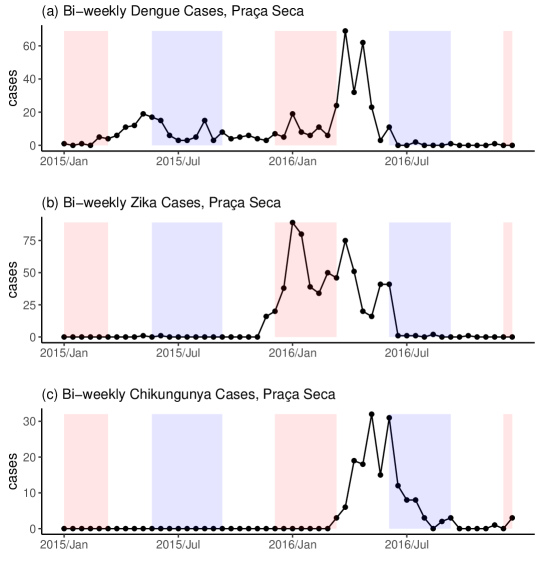
A potential issue with applying a multinomial model to multivariate spatio-temporal infectious disease counts is that many infectious diseases, especially vector-borne diseases, can be absent for long periods of time in an area (Bartlett, 1957; Coutinho et al., 2006; Adams and Boots, 2010). This behavior is illustrated in Figure 1 which shows bi-weekly reported case counts of dengue, Zika and chikungunya in the western Rio neighborhood of Praça Seca, between 2015-2016. While dengue cases are reported consistently throughout the two years, very few Zika cases and no chikungunya cases are reported in the first year. These patterns are typical of most neighborhoods. If a disease is absent in an area, then there should be no chance of cases being reported. However, a multinomial model will always assign a positive probability to cases being reported, which may lead to many more zeroes in the counts than can be realistically produced by the fitted model (Koslovsky, 2023). Also, we do not want to compare the transmission dynamics of a present disease and an absent one as it would likely overestimate the favorability of the present disease.
To account for long periods of disease absence, we will place our proposed autoregressive multinomial model within a zero-inflated multinomial modeling framework (Zeng et al., 2022; Koslovsky, 2023). Zero-inflated multinomial models allow categories, in our case diseases, to be absent from observations. If a category is absent, its multinomial probability is fixed at 0. The presence of a category is usually treated as random and generated through an independent Bernoulli process (Koslovsky, 2023). While a zero-inflated multinomial model would allow diseases to be absent in areas, existing approaches have made two independence assumptions that are inappropriate for spatio-temporal infectious disease counts. Firstly, they have assumed that the multivariate counts are independent conditional on the present categories of each observation. Infectious disease counts usually exhibit a high amount of correlation across space and time due to disease transmission (Bauer and Wakefield, 2018). Secondly, past approaches assumed that if a category is present in one observation it does not affect whether that category or other categories are present in other observations (independence of categorical presence). If an infectious disease is present in an area, then it is more likely to be present in the next time period, as disease presence and absence are usually persistent (Coutinho et al., 2006). Also, the presence of one disease may affect whether other diseases are present due to potential disease interactions (Paul et al., 2008). Finally, due to between-area disease spread (Grenfell et al., 2001), the status of the disease in an area will affect its presence in neighboring areas.
To address the above issues, we first choose a baseline disease that is well-established in the region and assume it is always present. This avoids all diseases being absent in an area at once which would be impossible if the total number of cases were not 0. We assume all other diseases switch back and forth between periods of presence and absence in each area through a series of Markov chains. The Markov chains account for long periods of disease absence, disease interactions and covariates, including the prevalence of the diseases in neighboring areas. For the diseases present in an area together, we assume that the relative distribution of their cases follows our proposed space-time autoregressive multinomial model. The absent diseases always report 0 cases. The rest of this paper is organized as follows. Section 2 introduces our proposed autoregressive multinomial model for comparing the transmission dynamics of multiple infectious diseases in a space-time setting. Section 2.1 extends the model to incorporate zero inflation and deal with long periods of disease absence. Section 3 details our Bayesian inferential procedure which utilizes the forward filtering backward sampling (FFBS) algorithm of Chib (1996) for efficient inference. In Section 4, we apply our model to cases of dengue, Zika and chikungunya in Rio de Janeiro during the first triple epidemic there. We close with a general discussion in Section 5.
2 An Autoregressive Multinomial Model for Comparing Transmission Dynamics
Assume we have reported case counts for different infectious diseases across areas and time periods. Let represent the vector of case counts for all diseases in area during the time interval , where represents the reported case counts for disease . We will first present our model without zero inflation and then extend to the zero-inflated case in Section 2.1. Since we are mainly interested in comparing the diseases, we condition on the total number of cases and model using a multinomial distribution,
| (1) |
where and is the vector of all case counts reported in the previous time, giving the model an autoregressive structure. In (1), represents the expected relative distribution of the disease counts at time in area given the previous observed counts . If conditions in favor some diseases over others then the share of the favored diseases should grow relative to those less favored. Therefore, we model the relative odds as,
| (2) |
for , where we assume disease 1 is the baseline disease and we add 1 to the top and bottom to avoid dividing by zero, adding such constants is common in autoregressive count models (Liboschik et al., 2017; Fritz and Kauermann, 2022). The parameters and , assumed to be between 0 and 1, are meant to account for nonhomogeneous mixing (Wakefield et al., 2019). That is, as cases increase there tends to be a dampening effect on transmission as individuals avoid infection and governments implement interventions. In (2), , which we link to covariates below, is a parameter that represents the favorability of conditions for the transmission of disease relative to the baseline disease during . For instance, if () then we would expect the share of disease to grow (shrink) relative to the baseline disease in , after adjusting for nonhomogeneous mixing with and . If , like for our motivating example in Section 4, then this means that if the share of disease will grow initially from an equal share. However, as disease becomes more dominant the share will be pulled back towards equality as individuals avoid infection from the dominant disease.
We link to covariates and random effects using a log-linear model,
| (3) |
where is a normal random intercept meant to account for between area differences and is a vector of covariates that might affect the favorability of disease relative to the baseline disease. We model the random effects using a multivariate normal distribution (Xia et al., 2013; Zeng et al., 2022),
| (4) |
where is a by variance-covariance matrix. These random effects are mainly meant to account for overdispersion, which is a very common issue when modeling multinomial counts (Xia et al., 2013). They also allow for a more flexible correlation structure between the individual disease counts, see the supplementary materials (SM) Section 2.
There is an epidemiological interpretation of the parameters in Equations (1)-(4). As we show in SM Section 1, if all diseases follow a Reed-Frost chain binomial SIR model (Abbey, 1952; Vynnycky, 2010; Bauer and Wakefield, 2018) with roughly the same serial interval, the time between successive generations of cases, then we can derive Equations (1)-(4). Under this derivation, in (2) represents the ratio of the effective reproduction number of disease and the baseline disease. The effective reproduction number is an important measure of transmission in epidemiology that gives the average number of new infections produced by a single infectious individual in the current population before they recover (Vynnycky, 2010). The covariate effect then represents the difference between the effect of covariate on the effective reproduction number of disease k and the baseline disease, see SM Section 1 for more details.
While the Reed-Frost model is commonly used (Wakefield et al., 2019), it makes assumptions that are not appropriate for many diseases (Abbey, 1952), and the model can be sensitive to underreporting and reporting delay when it comes to estimating the effective reproduction number (Bracher and Held, 2021; Quick et al., 2021). Regardless, the Reed-Frost derivation does reveal an important source of potential confounding due to differences in the susceptible populations, i.e., the population of individuals who are not immune to the disease. From the Reed-Frost derivation, see SM Equation (8), ideally, we would add to in Equation (3), where is the size of the susceptible population for disease in area at time . This makes sense intuitively, if a disease has a larger susceptible population compared to another then transmission for that disease will naturally be favored. The effect of any covariates correlated with the ratio of the susceptible populations could then be confounded. We conduct a sensitivity analysis to attempt to control for this for our motivating example in SM Section 8.
Finally, we note that the number of cases in neighboring areas may affect the favorability of the diseases as individuals will mix with those in neighboring areas (Grenfell et al., 2001). Therefore, we allow functions of disease cases in neighboring areas, such as the prevalence across neighboring areas, to be added to the covariate vector . Also, we allow previous counts of other diseases, e.g., for , to be added to to account for potential disease interactions (Freitas et al., 2019), see Section 4 for an example. We will call the model defined by (1)-(4) the autoregressive multinomial (ARMN) model.
2.1 Incorporating zero-inflation
As detailed in the introduction, if some of the diseases are absent in an area then the ARMN model is not appropriate as it will always assign a positive probability to cases being reported. In this subsection, we will keep the definitions from above and extend the ARMN model to deal with long periods of disease absence by adapting the proposal of Zeng et al. (2022) to our space-time setting. Let , for , be an indicator for the presence of disease , so that if disease was present in area during time and if disease was absent. Under the zero-inflated multinomial framework of Zeng et al. (2022), the multinomial probabilities are given by,
| (5) | ||||
for . An immediate issue with (5) is that we cannot have as we would divide by 0. Even if we were to define if , we would have the issue that this implies . A multinomial model conditions on the total count and does not generate it. There is nothing in the model of Zeng et al. (2022) to prevent . They may have overlooked this as they dealt with the case of and, therefore, it is very unlikely . However, in our motivating example, we have .
To prevent , as it makes sense in many epidemiological applications, we will assume that the baseline disease is well-established in the region and is always present. That is, we assume for all and . For instance, in our motivating example, dengue has been circulating in Rio since 1986 and is well-established there (Teixeira et al., 2009). We replace Equation (5) then by,
| (6) | ||||
for .
The presence of a disease in an area should depend on whether it was present previously, as disease presence and absence are often highly persistent (Coutinho et al., 2006; Douwes-Schultz and Schmidt, 2022), and may also depend on whether other diseases were present previously, as the diseases can interact with one another (Paul et al., 2008; Sherlock et al., 2013). Also, the presence of a disease might depend on environmental or socioeconomic factors, like temperature and water supply in the case of vector-borne diseases (Schmidt et al., 2011; Xu et al., 2017). Therefore, we model as,
| (7) | ||||
where is a vector of space-time covariates that might affect the presence of disease . As the disease may spread from neighboring areas (Grenfell et al., 2001), we allow functions of disease cases in neighboring areas to be added to , hence the dependence on in (7). For instance, the prevalence of the disease in neighboring areas could be added, see Section 4. Note, as in Equation (7) increases and decreases, the probability of getting a consecutive period of disease presence or absence approaches 1. Therefore, (7) can account for long consecutive periods of disease presence and absence which are often observed for infectious diseases, see Figure 1 and Coutinho et al. (2006).
We will call the ARMN model modified by Equations (6)-(7) the Markov switching zero-inflated autoregressive multinomial (MS-ZIARMN) model. Note, from Equation (6), for any possible values of the parameters and presence indicators. Also note that if diseases and are present in area during time we have , which is the same as in the ARMN model described in Equations (2)-(4). That is, the MS-ZIARMN model preserves the relative distribution of the present diseases from the ARMN model. Finally, if and we assume Equation (6), where and , we get the well known and popular zero-inflated binomial (ZIB) model of Hall (2000). Therefore, our model without space-time effects could be seen as a multinomial extension of Hall (2000).
3 Inferential Procedure
Here we assume the number of diseases is small enough for matrix multiplication with a by matrix to be computationally feasible. This should be the case in most epidemiological applications, for instance, in our motivating example we compare diseases. Our inferential strategy revolves around reparametrizing the MS-ZIARMN model as a Markov switching model (Frühwirth-Schnatter, 2006), which allows for very efficient Bayesian inference using the forward filtering backward sampling (FFBS) algorithm (Chib, 1996). To simplify the explanations we will assume, without loss of generality, that .
In the case of , we have as is always equal to 1. Let be an indicator for the possible values of , so that if , if , if and if . Then, from Equation (6),
| (8) |
meaning, for , the MS-ZIARMN model is a mixture of 4 different multinomial distributions where the multinomial probabilities are fixed at 0 for the diseases absent.
Note that, from Equation (7), as only depends on , and covariates, follows a first order nonhomogeneous Markov chain. Let be the transition matrix of , where for , and . As is an indicator for , the transition matrix can be derived through
for , using Equation (7). Finally, as depends on we require an initial distribution for the Markov chain, that is, for and . The modeler can set the initial distribution based on how likely they believe the diseases to be present at the beginning of the study period.
Given and for and , and for , we completely define a Markov switching model (Frühwirth-Schnatter, 2006). A Markov switching model assumes a time series can be described by several submodels, often called states or regimes, where switching between submodels is governed by a first-order Markov chain (Hamilton, 1989). In our case, the submodels are given by the 4 multinomial distributions in (8) and we switch between these submodels through the transition matrix . Typically, is called the state indicator.
Let be the vector of all state indicators, where , be the vector of all observations, and the vector of all parameters in the multinomial part of the model (see (2) and (4)); further, let be the vector of all parameters in the Markov chain part of the model (see (7)), and, finally, let be the vector of all model parameters. The likelihood of given and is given by,
| (9) |
Note, from Equation (8), is only fully known when , in which case we must have . It is possible, assuming is not too large, to use the forward filter (Hamilton, 1989) to completely marginalize from (9) and calculate , see SM Section 3. However, we want to make inferences about to investigate when the model believes the diseases were present or absent for model checking, see SM Section 5. Therefore, is estimated along with by sampling both from their joint posterior distribution , where is the prior distribution of . We specified wide independent priors for most lower-level elements of . We specified a conjugate inverse-Wishart prior for with degrees of freedom and identity matrix, as it implies the correlations in have marginal uniform prior distributions (Gelman et al., 2013).
As the joint posterior is not available in closed form, we resorted to Markov chain Monte Carlo (MCMC) methods, in particular, we used a hybrid Gibbs sampling algorithm with some steps of the Metropolis-Hastings algorithm to sample from it. The full details of the Gibbs sampler are given in SM Section 3. We sampled all of jointly from using the FFBS algorithm for Markov switching models (Chib, 1996). We found our MCMC algorithm mixed much faster when jointly sampling compared to sampling each presence indicator individually. This is typically the case for Markov switching models (Frühwirth-Schnatter, 2006) and was one of our main motivations for reparametrizing the MS-ZIARMN model as a Markov switching model.
Our MCMC algorithm was implemented using the R package Nimble (de Valpine et al., 2017). We implemented the FFBS algorithm using Nimble’s custom sampler feature. All other MCMC samplers mentioned in SM Section 3 are built into Nimble. All code and data are available on GitHub https://github.com/Dirk-Douwes-Schultz/MS_ZIARMN_code.
4 Application to Counts of Dengue, Zika and Chik.
Between 2015 and 2016 Rio de Janeiro experienced its first triple epidemic of dengue, Zika and chikungunya. Using space-time cluster analysis, Freitas et al. (2019) found that Zika and dengue clusters were much more likely in the western region of Rio (there were no chikungunya clusters found in the west), while other regions contained many clusters of each disease though they often differed in time. However, they did not investigate how these differences in clustering might depend on covariates or other factors. Schmidt et al. (2022), using a spatial multinomial regression model, found that cases of chikungunya were more likely in urban areas and Zika cases were less likely in population-dense areas, compared to dengue cases. A spatial analysis cannot investigate how space-time factors might have affected differences in the transmission intensity of the diseases, which may be important in this example, see below. Therefore, we apply our MS-ZIARMN model to cases of the three diseases, , across the 160 neighborhoods of Rio de Janeiro, , for each bi-week between 2015-2016, . Our model seems appropriate for this example as there appear to be long periods of disease absence in both the time series of chikungunya and Zika cases, see Figure 1 for example (overall 65% of Zika cases are equal to 0 and 75% of chikungunya cases are equal to 0).
4.1 Model specification and fitting
We modeled the Rio data with a bi-weekly time step as this roughly corresponds to the serial interval of the three diseases (Majumder et al., 2016; Riou et al., 2017). As mentioned in Section 2.1, we took dengue as the baseline disease (k=1) since it is well-established in the city and cases are reported consistently throughout the study period. We then considered to represent Zika and to represent chikungunya.
For in (3), covariates that may affect the favorability of Zika or chikungunya transmission relative to dengue transmission, we first took all spatial covariates considered in Schmidt et al. (2022): the percentage of neighborhood covered in green area, ; the social development index of neighborhood , ; and the population density of neighborhood , . We additionally considered the percentage of neighborhood that was occupied by favelas (slums), . These spatial covariates were chosen as the transmission of arboviral diseases can be significantly influenced by socioeconomic factors such as water supply and urbanicity (Schmidt et al., 2011), see Schmidt et al. (2022) for more details. As for space-time covariates, we first took the average weekly maximum temperature in neighborhood during bi-week , . Temperature is an important factor to consider since if the transmission of Zika or chikungunya is more sensitive (less sensitive) to temperature compared to dengue then their range of spread will be smaller (bigger) (Tesla et al., 2018; Mercier et al., 2022). Note, if there are many more cases of Zika or chikungunya in neighboring areas, compared to dengue, then we would expect the share of those diseases to grow all else equal, due to between-area mixing (Stoddard et al., 2013). Therefore, we considered the previous prevalence of disease and disease (dengue) across neighboring areas, and , in , where is the set of neighboring areas of neighborhood and is the population of neighborhood . We considered two areas neighbors if they shared a border. To simplify the model, we assumed the effect of neighboring dengue prevalence was the same on both and , like with the within-area autoregression. Finally, it was speculated in Freitas et al. (2019) that Zika circulation could have been inhibiting chikungunya transmission. To account for these kinds of disease interactions, we considered in and in . That is, chikungunya cases were allowed to affect the favorability of Zika transmission relative to dengue transmission and Zika cases were allowed to affect the favorability of chikungunya transmission relative to dengue transmission.
As for covariates potentially associated with the presence of Zika or chikungunya, in (7), we considered mostly the same factors included in . An exception is that we did not include the cases of the other disease as the Markov chain defined in (7) already accounts for disease interactions through . Also, since the presence is not defined relatively, we did not include neighboring dengue prevalence.
We also need to specify the initial state distributions, see Section 3. As there were no chikungunya cases reported at all in the first year, we assumed chikungunya had only a 5 percent chance of being present at the start of 2015. For Zika, there are a few, but not many, cases reported through most of 2015 and, therefore, we assumed a 10 percent chance of initial presence. We fitted the MS-ZIARMN model specified above to the Rio data using our proposed Gibbs sampler from Section 3. We ran the Gibbs sampler for 250,000 iterations on three chains with an initial burn-in of 50,0000 iterations. All sampling was started from random values in the parameter space to avoid convergence to local modes. Convergence was checked using the Gelman-Rubin statistic (1.05), the minimum effective sample size (1000) and by visually examining the traceplots (Plummer et al., 2006).
For comparison purposes, we also considered a model without zero inflation to ensure there is justification for treating the many zeroes in the data, as hypothesized. That is, the ARMN model described in Equations (1)-(4) with the same covariates and as the MS-ZIARMN model. We also considered a zero-inflated model without the coupled Markov chains, that is, with and for all and in Equation (7), which we will call the ZIARMN model. Without the coupled Markov chains, our model is a finite mixture and not a Markov mixture model, and the inference is greatly simplified, e.g., there is no need to use the FFBS algorithm. Finally, we compared with the zero-inflated multinomial model of Zeng et al. (2022) as our approach is built on their framework. Zeng et al. (2022) assumed that the probability a category was absent from an observation only depended on the category, so we let for in Equation (7). We kept the rest of the model the same as the MS-ZIARMN model. Note, Zeng et al. (2022) did not consider any covariates or space-time structure in the multinomial probabilities. However, this is inappropriate for our example and did not fit the data well (results not shown). Also, Zeng et al. (2022) did not assume the baseline category was always present, however, this appears to be necessary when modeling a small number of categories, see Section 2.1.
Table 1 shows the widely applicable information criterion (WAIC) (Gelman et al., 2014) of the 4 considered models. We calculated the WAIC by marginalizing out the state indicators as recommended by Auger-Méthé et al. (2021), see SM Section 4 for more details. Note, the model with the smallest WAIC is considered to have the best fit and as a rule of thumb a difference of 5 or more in the WAIC is considered significant. Table 1 shows it is not only important to account for zero inflation, but also covariates and correlations across space, time and disease in the zero-inflated process (i.e., the process of disease presence). Indeed, the model of Zeng et al. (2022) had a worse fit compared to the ARMN model (without zero inflation), despite the other zero-inflated models having a much better fit.
| Model | Zeng (2022) | ARMN | ZIARMN | MS-ZIARMN |
| WAIC | 23,986 | 23,974 | 22,756 | 22,091 |
4.2 Results
Table 2 shows the estimated coefficients from the multinomial part of the fitted MS-ZIARMN model, that is the intercepts and covariate effects from Equation (3). From the intercept row, at average values of the covariates, Zika transmission was favored over dengue and chikungunya transmission. That is, under average conditions the share of Zika cases tended to grow over time in an area (at least from an equal share, see the nuances in Section 2). It is interesting to compare these estimated intercepts with those from the ARMN and Zeng (2022) models in SM Table 1. Unlike the MS-ZIARMN model, the Zeng (2022) and ARMN models both estimated that on average Zika and chikungunya transmission was much less intense in Rio compared to dengue transmission. This does not correspond to our knowledge of the epidemiology of these diseases and is likely due to a failure to properly account for the many zeroes. Zika is generally considered more transmisable due to Ae. aegypti transmitting Zika at a higher rate (Freitas et al., 2019). This further illustrates it is important to account for zero inflation and to model the zero inflation properly (e.g., account for correlations).
| Relative Odds Ratio or Rate Ratio | ||
| Covariates | Zika-dengue | chik.-dengue |
| Intercept | 1.14 (1.03, 1.26) | 1.02 (.91, 1.13) |
| 1.02 (.95, 1.09) | .92 (.85, 1) | |
| 1.07 (.99, 1.15) | 1.01 (.92, 1.11) | |
| 1.02 (.94, 1.11) | 1.06 (.96, 1.16) | |
| .98 (.91, 1.05) | .94 (.87, 1.03) | |
| 1.14 (1.09, 1.20) | .85 (.80, .90) | |
| Neighborhood dengue prevalence | .70 (.67, .74) | .70 (.67, .74) |
| Neighborhood Zika prevalence | 1.59 (1.48, 1.70) | – |
| Neighborhood chik. prevalence | – | 1.43 (1.36, 1.50) |
| Previous Zika cases | – | .90 (.85, .96) |
| Previous chik. cases | .98 (.95, 1.02) | – |
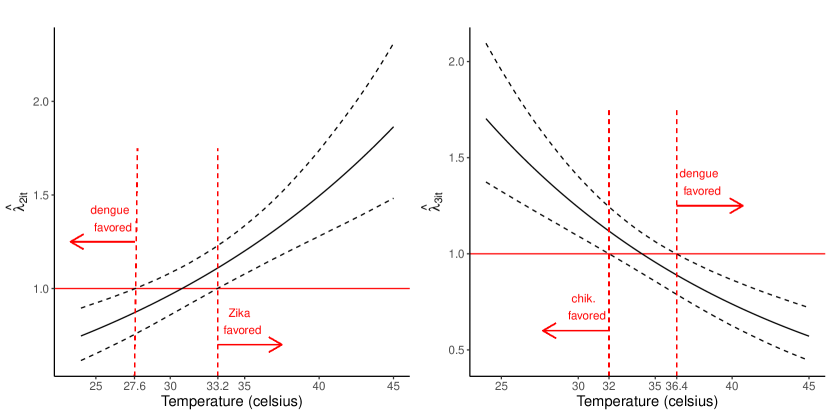
Interestingly, unlike in Schmidt et al. (2022), we did not find strong evidence that any of the spatial covariates were important for explaining differences in the transmission of the diseases. We found that Zika transmission was favored at warmer temperatures and chikungunya transmission was favored at colder temperatures, compared to dengue transmission. Both of these findings have been observed in laboratory studies (Tesla et al., 2018; Mercier et al., 2022). Indeed, a concern of chikungunya is that it could spread into colder areas of Europe unreachable by dengue (Mercier et al., 2022). To better quantify the temperature effects, we plot , from Equation (2), versus temperature for (Zika) and (chikungunya) in Figure 2. From the figure, we have strong evidence, under otherwise average conditions, that Zika transmission was favored above 33.2 degrees and chikungunya transmission was favored below 32 degrees, compared to dengue transmission.
The neighborhood prevalence effects are by far the strongest in Table 2 for explaining differences in the relative distribution of the diseases. For instance, we estimated that a standard deviation increase in the log of the prevalence of Zika across neighboring areas during the previous week was associated with a 59 (48, 70) percent increase in the odds of a new case being Zika relative to dengue. As Aedes aegypti primarily bite during the day, its arboviruses can spread rapidly between areas (Stoddard et al., 2013). We found that areas with more Zika cases were less favorable towards the transmission of chikungunya compared to dengue. That is, we estimated that a standard deviation increase in the log of the previous number of Zika cases in an area was associated with a 10 (4, 15) percent decrease in the odds of a new case being chikungunya relative to dengue. This does not necessarily mean that Zika transmission inhibited chikungunya transmission in a non-relative sense. It could be that Zika transmission encouraged both dengue and chikungunya transmission but the effect on dengue transmission was larger. Therefore, this result needs to be interpreted with some caution.
We estimated , and , from Equation (2), as .44 (.38, .49), .36 (.31, .32) and .43 (.36, .51) respectively, indicating a high degree of nonhomogeneous mixing. That is, the model predicts that if one of the diseases becomes very dominant in a neighborhood the relative distribution of the diseases will move towards a uniform distribution, perhaps because individuals avoid infection from the dominant disease. However, as avoiding one of the diseases should help avoid the others, as they are transmitted by the same vector, could also be mainly reflecting differences in disease immunity, which are hard to account for explicitly, see SM Section 8. From Equations (3)-(4), we estimated the standard deviation of as .75 (.71, .79), of as .80 (.75, .86) and the correlation between and as .59 (.52, .65). This implies that the correlation between the disease cases, marginalizing the random effects and conditional on their total, is about what we would expect without the random effects, see the simulation study in SM Section 2. That is, the random effects do not induce any excess correlation between the disease counts. However, they do induce a large amount of overdispersion, see Figure 4.
| Odds Ratio | Untransformed | |
| Covariate | Zika presence | chik. presence |
| Intercept | .1 (.08, .12) | -9.06 (-11.97, -7) |
| 1.14 (.98, 1.31) | 08 (-.20 .37) | |
| 1.11 (.96, 1.29) | .12 (-.18, .42) | |
| 1 (.85, 1.19) | .02 (-.33, .37) | |
| 1.03 (.89, 1.19) | 0 (-.3, .29) | |
| 1.44 (1.24, 1.66) | 1.11 (.6, 1.7) | |
| Neighborhood Zika prevalence | 1.70 (1.55, 1.87) | – |
| Neighborhood chik. prevalence | – | 1.09 (.85, 1.35) |
| Previous Zika presence | 6.41 (3.95, 9.94) | 5.12 (3.2, 8) |
| Previous chik. presence | 3.46 (2.42, 4.98) | 11.55 (8.13, 16.12) |
Table 3 shows the estimated parameters from the Markov chain component of the model, that is, from Equation (7). The Zika column shows the ratio of the odds of Zika presence corresponding to a unit increase in the covariate. However, the intercept for chikungunya is highly negative making the odds ratios difficult to interpret and, therefore, we did not transform the chikungunya estimates. From the intercept row, chikungunya was very unlikely to emerge in an area under average conditions. Indeed, chikungunya emergence was only likely after Zika had emerged and temperatures rose in the next summer. In contrast, the emergence of Zika was much more random, occurring with a 10 (8, 12) percent chance bi-weekly under average conditions. Once chikungunya did emerge it was likely to stay in the area (probability of .88 (.63, .99) assuming no neighboring cases, no Zika presence in the previous bi-week and otherwise average conditions). Both Zika and chikungunya were more likely to be present at high temperatures and when there were cases in neighboring areas. The effects of the neighborhood prevalences are especially large, again illustrating the disease’s high rate of geographical spread. Zika presence was an indicator for chikungunya presence and chikungunya presence was an indicator for Zika presence. This could be unrelated to disease interactions and due to unmeasured confounding as the diseases share the same vector.
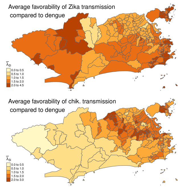
The maps in Figure 3 show the posterior mean of (average value of when disease was present in neighborhood ) for (Zika) (top map) and (chik.) (bottom map). From the bottom map, chikungunya transmission was disfavored in the west of the city when it was present, and the share of chikungunya cases tended to decline there. This was partly due to temperatures being 2-3 degrees higher on average in the west, see SM Figure 2, and chikungunya transmission being favored at colder temperatures relative to the other two diseases, see Table 2. Also, there were many Zika cases in the west of the city, and chikungunya transmission was disfavored in areas with many Zika cases. Zika transmission was favored throughout most of the city when it was present. This can be partly explained by the inherent favorability of Zika, i.e., the intercept in Table 2; temperatures typically being higher in Rio when Zika was present (the temperature covariate was centered using the overall average temperature) and Zika transmission being favored at higher temperatures.
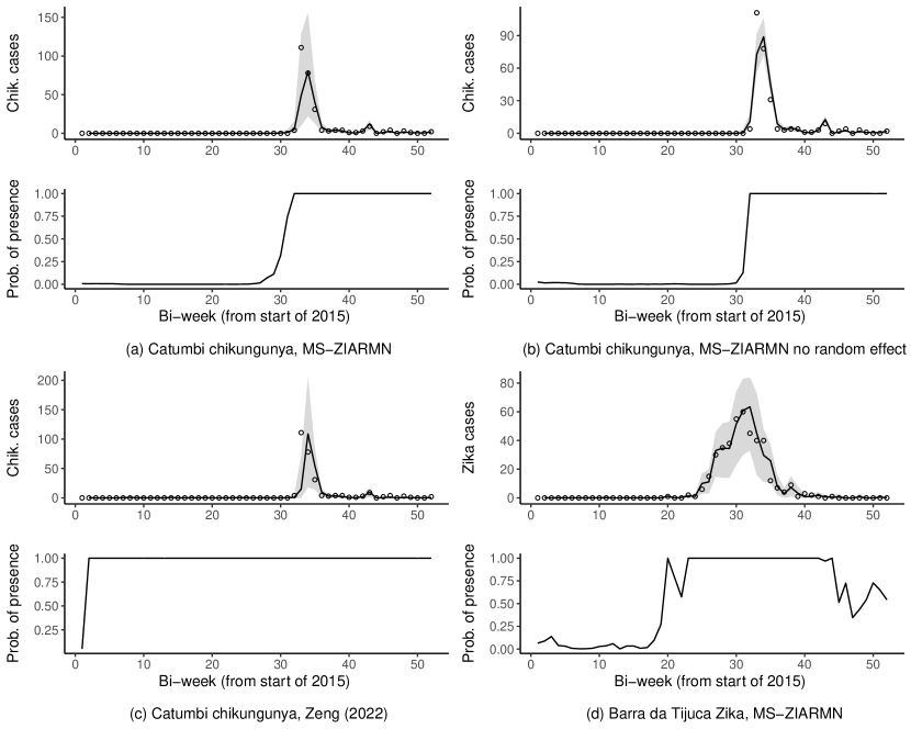
Figure 4 shows fitted values and posterior probabilities of disease presence, (see SM Section 5), from three models. SM Section 5 explains how we constructed the fitted values by drawing new space-time random effects and simulating from the fitted model. By comparing panels (a) and (b), the random effects , from Equations (3)-(4), are an important component of the model and induce a large amount of necessary overdispersion. From panel (c), the model of Zeng et al. (2022), which does not account for correlations in disease presence across space, time and disease, estimates chikungunya as always present in Catumbi, except for the initial state (this is also true for Zika and in all other areas). Therefore, the model of Zeng et al. (2022) is too restrictive to produce the likely complex space-time distribution of disease presence in the city. Comparing panels (a) and (d) shows the MS-ZIARMN model believes the presence of chikungunya was much more persistent compared to Zika, which follows the last two rows of Table 3. One way to think of (from the bottom graphs) is as a weight for the observation’s contribution to the likelihood of the multinomial parameters of the model. For example, from panel (a), the MS-ZIARMN model does not use any chikungunya observations before around week 28 in Catumbi to inform the multinomial estimates in Table 2. In contrast, the model of Zeng et al. (2022), from panel (c), will use all observations to inform the multinomial model which likely causes bias due to the large number of 0s, see the discussion at the beginning of Section 4.2.
The model takes disease absence to mean there was no chance of cases being reported. However, if the diseases are present in very small amounts, the chance of cases being reported could be close enough to 0 that it is indistinguishable. Indeed, if we replaced the 0s in Equation (8) by say .005, and normalized the probabilities, we would likely get similar parameter estimates. Therefore, disease presence should be interpreted closer to "a feasible chance of cases being reported" than "the presence of at least one infection".
5 Discussion
We have proposed a zero-inflated spatio-temporal multinomial model for comparing the transmission dynamics of multiple co-circulating infectious diseases. Our approach can account for long periods of disease absence while investigating how certain factors are related to differences in the transmission intensity of the diseases. Past zero-inflated multinomial models (Tang and Chen, 2019; Zeng et al., 2022; Koslovsky, 2023) have made independence assumptions that are inappropriate for spatio-temporal infectious disease counts, such as assuming categorical presence was independent between observations. We accounted for correlations across space, time and disease, in both the multinomial and zero-inflated components, through a combination of autoregression, regressing on past observations, and assuming the presence of the diseases followed a series of coupled Markov chains. This approach allowed for efficient and computationally feasible Bayesian inference using the FFBS algorithm.
We assume that the cases of the diseases present in an area jointly follow a multinomial model, conditioning on their total. It is more standard in the disease mapping literature to jointly model multiple disease counts with some form of a multivariate Poisson distribution (Jack et al., 2019). There are advantages to both approaches and we give a more detailed comparison of the two (without model fitting) in SM Section 1.2. If one is only interested in comparing the transmission of the diseases, like here, then a multinomial model eliminates many nuisance parameters and any shared space-time factors. A multivariate Poisson approach could estimate the overall effects of a covariate on transmission, not just the relative effects, and does not need to assume one of the diseases is always present. To the best of our knowledge, only Pavani and Moraga (2022) and Rotejanaprasert et al. (2021) have considered zero-inflated spatio-temporal multivariate Poisson models. Both relied on random effects to capture correlations in the data. However, these proposals have some important limitations, including not considering any space-time or space-time-disease interactions and not allowing the probability of disease presence to change over time. These modeling assumptions are inappropriate for our motivating example, and likely others, see Figure 4 for instance. An approach based on random effects could become intractable as one would need to consider random effects correlated across three dimensions, space, time and disease, in both the count and zero-inflated components of the model. Our approach seems much more computationally feasible and could be easily extended to the multivariate Poisson case, see SM Section 1.2. We will focus on these extensions and comparisons with the multinomial model in future work.
In our application, we found that Zika generally had more intense transmission compared to dengue and chikungunya, but was also not able to transmit as well at a lower temperature. This was not a major factor in tropical Rio, see Figure 3, but could be important in North America and Europe. In contrast, chikungunya transmission was relatively higher at lower temperatures meaning it might fare better in colder regions compared to Zika and dengue. Laboratory studies have come to similar conclusions (Tesla et al., 2018; Mercier et al., 2022). Alternative models that did not account for zero inflation or did not model correlations in disease presence (Zeng et al., 2022) did not fit as well and produced estimates inconsistent with our knowledge about the epidemiology of the diseases.
There are also some important limitations to our work. Being an observational study, unmeasured confounding could be an important issue, especially concerning differences in the susceptible populations which are unobservable. We tried using differences in cumulative incidence as a proxy for differences in the susceptible populations, in a sensitivity analysis in SM Section 8, and our results did not change. However, differences in cumulative incidence could be an imperfect proxy due to, for example, changes in reporting rates across space and time. Another limitation is that climate covariates, such as temperature, can have lagged and non-linear effects on the transmission of arboviral diseases (Lowe et al., 2018). As our multinomial model estimates differences in effects on transmission, our approach might be somewhat robust to non-linearity if the non-linear patterns are similar between diseases. It would be challenging to incorporate non-linear and lagged effects into our already complex modeling scheme. Shrinkage methods could help deal with the many parameters that would need to be added to the model by eliminating unimportant effects (Wang et al., 2023).
Acknowledgements
This work is part of the PhD thesis of D. Douwes-Schultz under the supervision of A. M. Schmidt in the Graduate Program of Biostatistics at McGill University, Canada. Douwes-Schultz is grateful for financial support from IVADO and the Canada First Research Excellence Fund/Apogée (PhD Excellence Scholarship 2021-9070375349). Schmidt is grateful for financial support from the Natural Sciences and Engineering Research Council (NSERC) of Canada (Discovery Grant RGPIN-2017-04999). This research was enabled in part by support provided by Calcul Québec (www.calculquebec.ca) and Compute Canada (www.computecanada.ca).
References
- Abbey (1952) Abbey, H. (1952) An examination of the Reed-Frost theory of epidemics. Human Biology, 24, 201–233.
- Adams and Boots (2010) Adams, B. and Boots, M. (2010) How important is vertical transmission in mosquitoes for the persistence of dengue? Insights from a mathematical model. Epidemics, 2, 1–10.
- Auger-Méthé et al. (2021) Auger-Méthé, M., Newman, K., Cole, D., Empacher, F., Gryba, R., King, A. A. et al. (2021) A guide to state–space modeling of ecological time series. Ecological Monographs, 91, e01470.
- Bartlett (1957) Bartlett, M. S. (1957) Measles periodicity and community size. Journal of the Royal Statistical Society: Series A (General), 120, 48–60.
- Bauer and Wakefield (2018) Bauer, C. and Wakefield, J. (2018) Stratified space–time infectious disease modelling, with an application to hand, foot and mouth disease in China. Journal of the Royal Statistical Society Series C (Applied Statistics), 67, 1379–1398.
- Bisanzio et al. (2018) Bisanzio, D., Dzul-Manzanilla, F., Gomez-Dantés, H., Pavia-Ruz, N., Hladish, T. J., Lenhart, A. et al. (2018) Spatio-temporal coherence of dengue, chikungunya and Zika outbreaks in Merida, Mexico. PLOS Neglected Tropical Diseases, 12, e0006298.
- Bracher and Held (2021) Bracher, J. and Held, L. (2021) A marginal moment matching approach for fitting endemic-epidemic models to underreported disease surveillance counts. Biometrics, 77, 1202–1214.
- Bradley et al. (2019) Bradley, J. R., Wikle, C. K. and Holan, S. H. (2019) Spatio-temporal models for big multinomial data using the conditional multivariate logit-beta distribution. Journal of Time Series Analysis, 40, 363–382.
- Cargnoni et al. (1997) Cargnoni, C., Müller, P. and West, M. (1997) Bayesian forecasting of multinomial time series through conditionally Gaussian dynamic models. Journal of the American Statistical Association, 92, 640–647.
- Chib (1996) Chib, S. (1996) Calculating posterior distributions and modal estimates in Markov mixture models. Journal of Econometrics, 75, 79–97.
- Coutinho et al. (2006) Coutinho, F. A. B., Burattinia, M. N., Lopeza, L. F. and Massada, E. (2006) Threshold conditions for a non-autonomous epidemic system describing the population dynamics of dengue. Bulletin of Mathematical Biology, 68, 2263–2282.
- Dabney and Wakefield (2005) Dabney, A. R. and Wakefield, J. C. (2005) Issues in the mapping of two diseases. Statistical Methods in Medical Research, 14, 83–112.
- Douwes-Schultz and Schmidt (2022) Douwes-Schultz, D. and Schmidt, A. M. (2022) Zero-state coupled Markov switching count models for spatio-temporal infectious disease spread. Journal of the Royal Statistical Society: Series C (Applied Statistics), 71, 589–612.
- Dreassi (2007) Dreassi, E. (2007) Polytomous disease mapping to detect uncommon risk factors for related diseases. Biometrical Journal, 49, 520–529.
- Fokianos and Kedem (2003) Fokianos, K. and Kedem, B. (2003) Regression theory for categorical time series. Statistical Science, 18, 357–376.
- Freitas et al. (2019) Freitas, L. P., Cruz, O. G., Lowe, R. and Sá Carvalho, M. (2019) Space–time dynamics of a triple epidemic: dengue, chikungunya and Zika clusters in the city of Rio de Janeiro. Proceedings of the Royal Society B: Biological Sciences, 286, 20191867.
- Fritz and Kauermann (2022) Fritz, C. and Kauermann, G. (2022) On the interplay of regional mobility, social connectedness and the spread of COVID-19 in Germany. Journal of the Royal Statistical Society: Series A (Statistics in Society), 185, 400–424.
- Frühwirth-Schnatter (2006) Frühwirth-Schnatter, S. (2006) Finite Mixture and Markov Switching Models. Springer Series in Statistics. New York: Springer-Verlag.
- Gelman et al. (2013) Gelman, A., Carlin, J. B., Stern, H. S., Dunson, D. B., Vehtari, A. and Rubin, D. B. (2013) Bayesian Data Analysis. Boca Raton: Chapman and Hall/CRC, 3rd edn.
- Gelman et al. (2014) Gelman, A., Hwang, J. and Vehtari, A. (2014) Understanding predictive information criteria for Bayesian models. Statistics and Computing, 24, 997–1016.
- Grenfell et al. (2001) Grenfell, B. T., Bjørnstad, O. N. and Kappey, J. (2001) Travelling waves and spatial hierarchies in measles epidemics. Nature, 414, 716–723.
- Hall (2000) Hall, D. B. (2000) Zero-inflated Poisson and binomial regression with random effects: A case study. Biometrics, 56, 1030–1039.
- Hamilton (1989) Hamilton, J. D. (1989) A new approach to the economic analysis of nonstationary time series and the business cycle. Econometrica, 57, 357–384.
- Jack et al. (2019) Jack, E., Lee, D. and Dean, N. (2019) Estimating the changing nature of Scotland’s health inequalities by using a multivariate spatiotemporal model. Journal of the Royal Statistical Society Series A (Statistics in Society), 182, 1061–1080.
- Kazazian et al. (2020) Kazazian, L., Neto, A. S. L., Sousa, G. S., Nascimento, O. J. d. and Castro, M. C. (2020) Spatiotemporal transmission dynamics of co-circulating dengue, Zika, and chikungunya viruses in Fortaleza, Brazil: 2011–2017. PLoS Neglected Tropical Diseases, 14, e0008760.
- Koslovsky (2023) Koslovsky, M. D. (2023) A Bayesian zero-inflated Dirichlet-multinomial regression model for multivariate compositional count data. Biometrics, 79, 3239–3251.
- Liboschik et al. (2017) Liboschik, T., Fokianos, K. and Fried, R. (2017) Tscount: An R package for analysis of count time series following generalized linear models. Journal of Statistical Software, 82, 1–51.
- Loredo-Osti and Sutradhar (2012) Loredo-Osti, J. C. and Sutradhar, B. C. (2012) Estimation of regression and dynamic dependence paremeters for non-stationary multinomial time series. Journal of Time Series Analysis, 33, 458–467.
- Lowe et al. (2018) Lowe, R., Gasparrini, A., Meerbeeck, C. J. V., Lippi, C. A., Mahon, R., Trotman, A. R. et al. (2018) Nonlinear and delayed impacts of climate on dengue risk in Barbados: A modelling study. PLoS Medicine, 15, e1002613.
- Majumder et al. (2016) Majumder, M., Cohn, E., Fish, D. and Brownstein, J. (2016) Estimating a feasible serial interval range for Zika fever. Bulletin of the World Health Organization.
- Mercier et al. (2022) Mercier, A., Obadia, T., Carraretto, D., Velo, E., Gabiane, G., Bino, S. et al. (2022) Impact of temperature on dengue and chikungunya transmission by the mosquito Aedes albopictus. Scientific Reports, 12, 6973.
- Paul et al. (2008) Paul, M., Held, L. and Toschke, A. M. (2008) Multivariate modelling of infectious disease surveillance data. Statistics in Medicine, 27, 6250–6267.
- Pavani and Moraga (2022) Pavani, J. and Moraga, P. (2022) A Bayesian joint spatio-temporal model for multiple mosquito-borne diseases. In New Frontiers in Bayesian Statistics (eds. R. Argiento, F. Camerlenghi and S. Paganin), Springer Proceedings in Mathematics & Statistics, 69–77. Cham: Springer International Publishing.
- Pereira et al. (2018) Pereira, S., Turkman, F. and Correia, L. (2018) Spatio-temporal analysis of regional unemployment rates: A comparison of model based approaches. Revstat - Statistical Journal, 16, 515–536.
- Plummer et al. (2006) Plummer, M., Best, N., Cowles, K. and Vines, K. (2006) CODA: Convergence diagnosis and output analysis for MCMC. R News, 6, 7–11.
- Quick et al. (2021) Quick, C., Dey, R. and Lin, X. (2021) Regression models for understanding COVID-19 epidemic dynamics with incomplete data. Journal of the American Statistical Association, 116, 1561–1577.
- Riou et al. (2017) Riou, J., Poletto, C. and Boëlle, P.-Y. (2017) A comparative analysis of chikungunya and Zika transmission. Epidemics, 19, 43–52.
- Rodriguez-Morales et al. (2016) Rodriguez-Morales, A. J., Villamil-Gómez, W. E. and Franco-Paredes, C. (2016) The arboviral burden of disease caused by co-circulation and co-infection of dengue, chikungunya and Zika in the Americas. Travel Medicine and Infectious Disease, 14, 177–179.
- Rotejanaprasert et al. (2021) Rotejanaprasert, C., Lee, D., Ekapirat, N., Sudathip, P. and Maude, R. J. (2021) Spatiotemporal distributed lag modelling of multiple Plasmodium species in a malaria elimination setting. Statistical Methods in Medical Research, 30, 22–34.
- Schmidt et al. (2022) Schmidt, A. M., Freitas, L. P., Cruz, O. G. and Carvalho, M. S. (2022) A Poisson-multinomial spatial model for simultaneous outbreaks with application to arboviral diseases. Statistical Methods in Medical Research, 31, 1590–1602.
- Schmidt et al. (2011) Schmidt, W.-P., Suzuki, M., Thiem, V. D., White, R. G., Tsuzuki, A., Yoshida, L.-M. et al. (2011) Population density, water supply, and the risk of dengue fever in vietnam: Cohort study and spatial analysis. PLOS Medicine, 8, e1001082.
- Sherlock et al. (2013) Sherlock, C., Xifara, T., Telfer, S. and Begon, M. (2013) A coupled hidden Markov model for disease interactions. Journal of the Royal Statistical Society Series C (Applied Statistics), 62, 609–627.
- Sosa et al. (2023) Sosa, J., Briz-Redon, A., Flores, M., Abril, M. and Mateu, J. (2023) A spatio-temporal multinomial model of firearm death in Ecuador. Spatial Statistics, 54, 100738.
- Stoddard et al. (2013) Stoddard, S. T., Forshey, B. M., Morrison, A. C., Paz-Soldan, V. A., Vazquez-Prokopec, G. M. et al. (2013) House-to-house human movement drives dengue virus transmission. Proceedings of the National Academy of Sciences of the United States of America, 110, 994–999.
- Tang and Chen (2019) Tang, Z.-Z. and Chen, G. (2019) Zero-inflated generalized Dirichlet multinomial regression model for microbiome compositional data analysis. Biostatistics, 20, 698–713.
- Teixeira et al. (2009) Teixeira, M. G., Costa, M. d. C. N., Barreto, F. and Barreto, M. L. (2009) Dengue: twenty-five years since reemergence in Brazil. Cadernos de Saúde Pública, 25, S7–S18.
- Tepe and Guldmann (2020) Tepe, E. and Guldmann, J.-M. (2020) Spatio-temporal multinomial autologistic modeling of land-use change: A parcel-level approach. Environment and Planning B: Urban Analytics and City Science, 47, 473–488.
- Tesla et al. (2018) Tesla, B., Demakovsky, L. R., Mordecai, E. A., Ryan, S. J., Bonds, M. H., Ngonghala, C. N. et al. (2018) Temperature drives Zika virus transmission: evidence from empirical and mathematical models. Proceedings of the Royal Society B: Biological Sciences, 285, 20180795.
- de Valpine et al. (2017) de Valpine, P., Turek, D., Paciorek, C. J., Anderson-Bergman, C., Lang, D. T. and Bodik, R. (2017) Programming with models: Writing statistical algorithms for general model structures with NIMBLE. Journal of Computational and Graphical Statistics, 26, 403–413.
- Vynnycky (2010) Vynnycky, E. (2010) An Introduction to Infectious Disease Modelling. New York: Oxford University Press, USA, 1st edn.
- Wakefield et al. (2019) Wakefield, J., Dong, T. Q. and Minin, V. N. (2019) Spatio-temporal analysis of surveillance data. In Handbook of Infectious Disease Data Analysis (eds. L. Held, N. Hens, P. O’Neil and J. Wallinga), 455–475. Boca Raton: Chapman and Hall/CRC.
- Wang et al. (2023) Wang, E., Chiang, S., Haneef, Z., Rao, V., Moss, R. and Vannucci, M. (2023) Bayesian non-homogeneous hidden Markov model with variable selection for investigating drivers of seizure risk cycling. The Annals of Applied Statistics, 17, 333–356.
- Xia et al. (2013) Xia, F., Chen, J., Fung, W. K. and Li, H. (2013) A logistic normal multinomial regression model for microbiome compositional data analysis. Biometrics, 69, 1053–1063.
- Xu et al. (2017) Xu, L., Stige, L. C., Chan, K.-S., Zhou, J., Yang, J., Sang, S. et al. (2017) Climate variation drives dengue dynamics. Proceedings of the National Academy of Sciences, 114, 113–118.
- Zeng et al. (2022) Zeng, Y., Pang, D., Zhao, H. and Wang, T. (2022) A zero-inflated logistic normal multinomial model for extracting microbial compositions. Journal of the American Statistical Association, 118, 2356––2369.