Market Power Mitigation in Two-stage Electricity Markets with Supply Function and Quantity Bidding

Rajni Kant Bansal, Yue Chen, Pengcheng You, Enrique Mallada R. K. Bansal and E. Mallada are with the Johns Hopkins University, Baltimore, MD 21218, USA (email: {rbansal3,mallada}@jhu.edu)Y. Chen is with The Chinese University of Hong Kong, Shatin, Hong Kong SAR, China (email:[email protected])P. You is with the Peking University, Beijing, China (email:[email protected])This work was supported by NSFC (grants 72201007, T2121002, 72131001, 61973163, and 52307144) and NSF (grants CAREER ECCS 1752362, CPS ECCS 2136324, and Global Centers 2330450).

Abstract

Two-stage settlement electricity markets, which include day-ahead and real-time markets, often observe undesirable price manipulation due to the price difference across stages, inadequate competition, and unforeseen circumstances. To mitigate this, some Independent System Operators (ISOs) have proposed system-level market power mitigation (MPM) policies in addition to existing local policies. These system-level policies aim to substitute noncompetitive bids with a default bid based on estimated generator costs. However, without accounting for the conflicting interest of participants, they may lead to unintended consequences when implemented. In this paper, we model the competition between generators (bidding supply functions) and loads (bidding quantity) in a two-stage market with a stage-wise MPM policy. An equilibrium analysis shows that a real-time MPM policy leads to equilibrium loss, meaning no stable market outcome (Nash equilibrium) exists. A day-ahead MPM policy leads to Stackelberg-Nash game, with loads acting as leaders and generators as followers. Despite estimation errors, the competitive equilibrium is efficient, while the Nash equilibrium is comparatively robust to price manipulations. Moreover, analysis of inelastic loads shows their tendency to shift allocation and manipulate prices in the market. Numerical studies illustrate the impact of cost estimation errors, heterogeneity in generation cost, and load size on market equilibrium.

Index Terms:

electricity market, two-stage settlement, supply function bidding, Stackelberg game, equilibrium analysis

I Introduction

Most wholesale energy markets in the US consider a two-stage settlement system as a market norm, i.e., day-ahead and real-time markets. The first stage, the day-ahead (forward) market, clears a day before the delivery based on the hourly forecasts of resources for the next day and accounts for the majority of energy trades. The second stage, the real-time (spot) market, occurs at a faster timescale (typically every five minutes) and is considered a last resort for participants to adjust their commitment following forecast errors [1, 2]. The main goal of such a sequential two-stage market is to operate efficiently and encourage market participation. However, the often price difference between the two stages in practice, due to intrinsic uncertainty in the forecast, unscheduled maintenance, etc., creates opportunities for price speculation and arbitrage, which could be further exploited by strategic participants to their benefit [3, 4].

To discourage suppliers from exploiting consumers, most operators employ an inbuilt local market power mitigation mechanism (LMPM) triggered at congestion during market clearing [5, 6]. Despite this, some operators, like California Independent System Operator (CAISO), have documented periods of time with non-competitive bids (approximately $2\%$ hours in the case of CAISO [7]). It led to the development of initiatives aimed at implementing system-level market power mitigation (MPM), i.e., bid mitigation similar to LMPM, but system-wide for each stage separately [8, 9]. Such system-level policies, when implemented, substitute in, e.g., real-time or day-ahead, any non-competitive bids with default bids, which estimate generator costs based on the operator’s knowledge of technology, fuel prices, and operational constraints [10, §39.7.1],[11]. Although such market policies are straightforward, their effect on market outcome remains unknown if implemented without accounting for the conflicting interest of individual participants. This paper studies the proposed system-level policies and discusses the possible unintended effects.

Precisely, we study a sequential game formulation in a two-stage market with an MPM policy to analyze the competition between generators (bidding supply functions and seeking to maximize individual profit) [12] and loads (bidding demand quantities and minimizing payment) [13] such that the market operator substitutes generators’ bids with default bids as per the policy. In this paper, we assume that an operator makes an error in estimating the truthful cost of dispatching generators in a stage with an MPM policy. We show that a real-time MPM policy results in a loss of market equilibrium. However, the complimentary case of a day-ahead MPM policy leads to a form of Stackelberg-Nash game with loads leading generators in their decision-making. A detailed Nash equilibrium analysis for this case shows a stable market outcome that is comparatively robust to price manipulations.

The main contributions of this paper are summarized below:

1

We show that a real-time MPM policy leads to a Nash game in the day-ahead, while generators participate truthfully in real-time. We characterize the competitive equilibrium of such a game, which is inefficient w.r.t the social planner’s problem. Further, competition between price-anticipating participants does not result in a stable market outcome, and a Nash equilibrium does not exist.
2

We then study the impact of a day-ahead MPM policy that leads to a generalized Stackelberg-Nash game with loads acting as leaders in the day-ahead market and generators acting as followers in the real-time market. Despite the operator’s error in cost estimation, the competitive equilibrium of the resulting game is efficient. Also, the Nash equilibrium, assuming that generators are homogeneous and bid symmetrically for closed-form analysis, is robust to price manipulations compared to standard markets, i.e., a two-stage market without any mitigation policies.
3

To understand the impact of these policies, we compare the day-ahead MPM policy market equilibrium with the equilibrium in a standard market. The closed-form analysis shows that prices across stages are the same for the two cases. However, loads acting as leaders in a market with a day-ahead MPM policy allocates higher demand in day-ahead at the expense of generators’ profit. Despite being inelastic, loads can shift their allocation and manipulate prices in the market.
4

We further provide a detailed numerical study to illustrate the impact of a day-ahead MPM policy. We show that the Nash equilibrium converges to competitive equilibrium as the number of participants increases in the market. Overestimation of the cost of generators benefits them with a higher profit and helps mitigate the market power of loads. Furthermore, the case with heterogeneity in generator cost shows that expensive generators are least affected when benchmarked with the competitive equilibrium. The case with significant diversity in load participants reveals that a sufficiently smaller load could earn money instead of making payments at the expense of larger loads in the market.

Related work: Understanding market power and strategies for mitigating it has been an extensive subject of study in the literature. Prior works have studied the identification of market power [14, 15], the development of metrics to quantify it [16], competition between various market players[17, 18, 19], and general analysis of market power in two-stage markets [1, 20, 21, 22, 23]. In addition, some works have analyzed local MPM policies, e.g. see [24]. However, a closed-form analysis, where the system-level policy effect on the resulting equilibrium is studied counterfactually, is rare in the literature. Our work contributes to the field by conducting a counterfactual study on the impact of CAISO’s system-level policy based on default bids and the role of inelastic demand in the market. To the best of our knowledge, there is no existing study that investigates these features.

Paper Organization: The rest of the paper is structured as follows. In Section II we first introduce the social planner problem, two-stage market model, and participants’ behavior, and then define a two-stage market equilibrium. In Section III we model the market power mitigation policy for each stage, characterize the market equilibrium, and compare it with the solution to the social planner problem. We first compare the impact of MPM policies on market equilibrium and then compare it with a standard market equilibrium in Section IV. Numerical studies on market power for a day-ahead MPM policy, limitations of work along with policy implications, and conclusions are in Section V, VI, and VII, respectively.

Notation

We use standard notation $f(a,b)$ to denote a function of independent variables $a$ and $b$ . However, we use $f(a;b)$ to represent a function of independent variable $a$ and parameter $b$ .

II Market Model

In this section, we formulate the social planner problem and describe the standard two-stage settlement market. We then formally define participants’ behavior, i.e., price-taking or price-anticipating, and lay out a general market equilibrium.

II-A Social Planner Problem

Consider a single-interval two-stage settlement market where a set $\mathcal{G}$ of generators participate with a set $\mathcal{L}$ of inelastic loads to meet inelastic aggregate demand $d\in\mathbb{R}$ . Each generator $j\in\mathcal{G}$ supplies $g_{j}\in\mathbb{R}$ and each inelastic load $l\in\mathcal{L}$ consumes $d_{l}\in\mathbb{R}$ respectively, where $\sum_{l\in\mathcal{L}}d_{l}=d$ . We define $G:=|\mathcal{G}|$ and $L:=|\mathcal{L}|$ to denote the number of generators and loads, respectively. Assuming a quadratic cost function for the generators, the social planner problem — minimum cost of meeting aggregate inelastic demand — is given by


$\displaystyle\min_{g_{j},j\in\mathcal{G}}$	$\displaystyle\sum\nolimits_{j\in\mathcal{G}}\frac{c_{j}}{2}{g_{j}}^{2}$	(1a)
s.t.	$\displaystyle\sum\nolimits_{l\in\mathcal{L}}d_{l}=\sum\nolimits_{j\in\mathcal{G}}g_{j}$	(1b)

where (1b) enforces the power balance in the market.

II-B Two-Stage Market Mechanism

In this subsection, we define the two-stage market clearing, as shown in Figure 1. The net output $g_{j}$ of each generator $j$ and individual load $d_{l}$ of load $l$ is allocated over two stages, such that

\displaystyle g_{j}=g_{j}^{d}+g_{j}^{r},\ d_{l}^{d}+d_{l}^{r}=d_{l}

(2)

where $(g_{j}^{d},d_{l}^{d})$ and $(g_{j}^{r},d_{l}^{r})$ represent allocation in day-ahead and real-time markets, respectively.

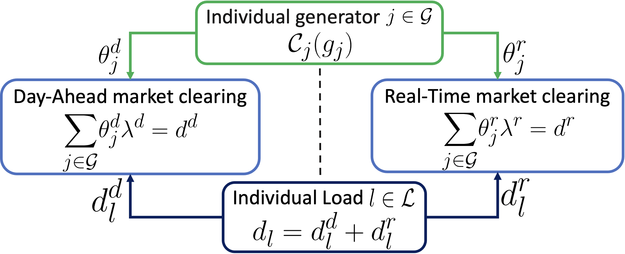
Refer to caption — Figure 1: Two-stage Market Mechanism

II-B1 Day-Ahead Market

The power output of each generator $j\in\mathcal{G}$ in the day-ahead market is denoted by $g_{j}^{d}$ . Each generator $j$ submits a supply function parameterized by the slope $\theta_{j}^{d}$ , that indicates willingness of generator $j$ to supply $g_{j}^{d}$ as a function of price

\displaystyle g_{j}^{d}=\theta_{j}^{d}\lambda^{d}

(3)

where $\lambda^{d}$ denotes the price in the day-ahead market. Each load $l\in\mathcal{L}$ bids quantity $d_{l}^{d}$ in the day-ahead market. Based on the bids $(\theta_{j}^{d},d_{l}^{d})$ from participants, the market operator clears the day-ahead market to meet the supply-demand balance.

\displaystyle\sum\nolimits_{j\in\mathcal{G}}\theta_{j}^{d}\lambda^{d}=d^{d}

(4)

The optimal solution to the day-ahead dispatch problem (4) gives the optimal dispatch $(g_{j}^{d},d_{l}^{d})$ and clearing prices $\lambda^{d}$ to all the participants. Each generator $j\in\mathcal{G}$ and load $l\in\mathcal{L}$ are paid $\lambda^{d}g_{j}^{d}$ and $\lambda^{d}d_{l}^{d}$ as part of the market settlement.

II-B2 Real-Time Market

The power output of each generator $j$ in real-time market is denoted by $g_{j}^{r}$ and their bid is:

\displaystyle g_{j}^{r}=\theta_{j}^{r}\lambda^{r}

(5)

where $\lambda^{r}$ denotes the price in the real-time market. The supply function bid is parameterized by $\theta_{j}^{r}$ , indicating willingness of generator $j$ to supply $g_{j}^{r}$ at the price $\lambda^{r}$ . Each load $l\in\mathcal{L}$ submits quantity bids $d_{l}^{r}$ . Given the bids $(\theta_{j}^{r},d_{l}^{r})$ , the operator clears the real-time market to meet the supply-demand balance.

\displaystyle\sum\nolimits_{j\in\mathcal{G}}\theta_{j}^{r}\lambda^{r}=d^{r}

(6)

Similar to the day-ahead market clearing, the optimal solution to the dispatch problem (6) gives the optimal dispatch and the market clearing prices $\lambda^{r}$ to all the participants, such that each generator $j\in\mathcal{G}$ and load $l\in\mathcal{L}$ produces or consumes $g_{j}^{r}$ and $d_{l}^{r}$ , and is paid or charged $\lambda^{r}g_{j}^{r}$ and $\lambda^{r}d_{l}^{r}$ , respectively.

II-B3 Market Rules and Goal

In this section, we first define a set of rules to account for degenerate cases in the market mechanism and then discuss the goal of a two-stage market.

Rule 1

For $v\in\{d,r\}$ and $w\in\{d,r\}$ , if the net supply and demand of the generators and loads in a stage follow

\displaystyle{\color[rgb]{0,0,0}\sum\nolimits_{j\in\mathcal{G}}\theta_{j}^{v}\lambda^{v}=0,\ d^{v}=0\implies\lambda^{v}=\lambda^{w},\ v\neq w}

(7)

i.e., the clearing price in that stage is set to the clearing prices of the other stage with a non-zero demand.

Rule 2

For $v\in\{d,r\}$ , if the net supply and net demand of the generators and loads in a stage follow

\displaystyle\sum\nolimits_{j\in\mathcal{G}}\theta_{j}^{v}\lambda^{v}=0,\ d^{v}\neq 0\implies\lambda^{v}=0

(8)

i.e., the clearing price is set to zero, and demand is split evenly across all the loads.

We are interested in two-stage market outcomes that satisfy

\displaystyle\sum\limits_{j\in\mathcal{G}}(g_{j}^{d}+g_{j}^{r})=\sum\limits_{j\in\mathcal{G}}g_{j}=\sum\limits_{l\in\mathcal{L}}(d_{l}^{d}+d_{l}^{r})=\sum\limits_{l\in\mathcal{L}}d_{l}=d

(9)

and solve the social planner problem (1). Though the market outcome may deviate from the optimal social planner solution, signaling efficiency losses due to price manipulation by participants, we quantify such deviations to understand the behavior of participants and the market outcome.

II-C Participant Behaviour

In this section, for the purposes of our study, we introduce two different types of rational participants’ behavior, price-taking, and price-anticipating. Each generator $j\in\mathcal{G}$ seeks to maximize their profit $\pi_{j}$ , given by:

\displaystyle\pi_{j}(g_{j}^{d},g_{j}^{r},\lambda^{d},\lambda^{r})\!:=\!\lambda^{r}g_{j}^{r}\!\!+\lambda^{d}g_{j}^{d}\!-\!\frac{c_{j}}{2}{g_{j}}^{2}

(10)

Each load $l\in\mathcal{L}$ aims to minimize their payments $\rho_{l}$ , as:

\displaystyle\rho_{l}(d_{l}^{d},d_{l}^{r},\lambda^{d},\lambda^{r}):=\lambda^{d}d_{l}^{d}+\lambda^{r}d_{l}^{r}

(11)

Substituting the load coupling constraint (2) in (11) we get,

\displaystyle\rho_{l}(d_{l}^{d},\lambda^{d},\lambda^{r}):=\lambda^{d}d_{l}^{d}+\lambda^{r}(d_{l}-d_{l}^{d})

(12)

For each load $l\in\mathcal{L}$ , the allocation in the day-ahead market $d_{l}^{d}$ determines its allocation in the real-time market $d_{l}^{r}$ due to the demand inelasticity.

II-C1 Price-Taking Participants

A price-taker participant is defined below:

Definition 1

A market participant is price-taking if it accepts the existing prices in the market and does not anticipate the impact of its bid on the market prices.

Given the prices in the day-ahead market $\lambda^{d}$ and real-time market $\lambda^{r}$ , the generator individual problem is given by:

\displaystyle\max_{g_{j}^{d},g_{j}^{r}}\ \pi_{j}(g_{j}^{d},g_{j}^{r};\lambda^{d},\lambda^{r})

(13)

Similarly given the prices $\lambda^{d},\lambda^{r}$ , the individual bidding problem for load is given by:

\displaystyle\min_{d_{l}^{d}}\

\displaystyle\rho_{l}(d_{l}^{d};\lambda^{d},\lambda^{r})

(14)

We next define the price-anticipating (or strategic) participants.

II-C2 Price-Anticipating Participants

A price-anticipating participant is defined below:

Definition 2

A market participant is price-anticipating (strategic) if it anticipates the impact of its bid on the prices in two stages and has complete knowledge of other participants’ bids.

The individual problem of a price-anticipating generator is:


		$\displaystyle\!\!\!\max_{g_{j}^{d},g_{j}^{r},\lambda^{d},\lambda^{r}}\ \!\pi_{j}\!\left(g_{j}^{d},g_{j}^{r},\lambda^{d}\!\left(g_{j}^{d};\overline{g}_{-j}^{d},d^{d}\right),\lambda^{r}\!\!\left(g_{j}^{r};\overline{g}_{-j}^{r},d^{r}\right)\right)$		(15a)
		$\displaystyle\textrm{ s.t. }\eqref{da_power_bal},\eqref{rt_power_bal}$		(15b)

where $\overline{g}_{-j}^{d}:=\sum_{k\in\mathcal{G},k\neq j}g_{k}^{d}$ , and $\overline{g}_{-j}^{r}:=\sum_{k\in\mathcal{G},k\neq j}g_{k}^{r}$ . The generator $j$ maximizes its profit while anticipating the market clearing prices in the day-ahead and real-time market (4),(6), along with complete knowledge of load bids $d_{l}^{d},d_{l}^{r},l\in\mathcal{L}$ , and other generators’ bids $\theta_{k}^{d},\theta_{k}^{r},k\in\mathcal{G},k\neq j$ . Similarly, the individual problem for strategic load $l$ with complete knowledge of prices in two stages (4),(6) and other participants’ bids:


	$\displaystyle\!\!\!\min_{d_{l}^{d},\lambda^{d},\lambda^{r}}\ \rho_{l}\!\left(d_{l}^{d},\lambda^{d}\!\left(d_{l}^{d};g_{j}^{d},\overline{d}_{-l}^{d}\right)\!\!,\lambda^{r}\!\!\left(d_{l}^{d};g_{j}^{r},\overline{d}_{-l}^{r}\right)\right)$		(16a)
	$\displaystyle\textrm{ s.t. }\eqref{da_power_bal},\eqref{rt_power_bal}$		(16b)

where the load $l$ minimizes its payment in the market and $\overline{d}_{-l}^{d}:=\sum_{l\in\mathcal{L},k\neq l}d_{l}^{d},\ \overline{d}_{-l}^{r}:=\sum_{l\in\mathcal{L},k\neq l}d_{l}^{r}$ .

II-D Market Equilibrium

In this section, for the purpose of this study, we characterize the market equilibrium in a two-stage settlement electricity market. At the equilibrium, no participant has any incentive to deviate from their bid, and market clears, as defined below.

Definition 3

We say the participant bids and market clearing prices $({\theta_{j}^{d}},{\theta_{j}^{r}},j\in\mathcal{G},d_{l}^{d},d_{l}^{r},l\in\mathcal{L},\lambda^{d},\lambda^{r})$ in the day-ahead and real-time respectively form a two-stage market equilibrium if the following conditions are satisfied:

1.

For each generator $j\in\mathcal{G}$ , the bid $\theta_{j}^{d},\theta_{j}^{r}$ maximizes their individual profit.
2.

For each load $l\in\mathcal{L}$ , the allocation $d_{l}^{d},d_{l}^{r}$ minimizes their individual payment.
3.

The inelastic demand $d\in\mathbb{R}$ is satisfied with the market-clearing prices $\lambda^{d}$ given by (4) and $\lambda^{r}$ given by (6) over the two-stages of the market.

We will study market equilibria as a tool to understand the impact of MPM policies.

III Understanding Impact of MPM Policy

In this section, we first characterize the market equilibrium in a standard two-stage market without any such mitigation policy [1], then model mitigation policies and the resulting market equilibrium. In particular, ISOs have significant prior knowledge of market participants allowing them to evaluate the competitiveness of energy bids. For example, operators are aware of the generator’s technology, fuel prices, and operational constraints that can be used to estimate or bound the generator’s cost [10, §39.7.1],[11] within a reasonable threshold under the mitigation policies. We assume that the operator makes an error in estimating the truthful cost of dispatching the generator in a stage with a mitigation policy.

III-A Standard Two-stage Market

The role of participants in a standard market without any mitigation policy is studied extensively in the literature [25, 12, 26, 1]. Here, we cite the results from [1] that analyze the role of strategic generators and inelastic demand in a standard two-stage market and use them as a benchmark to analyze the impact of a mitigation policy in the market.

III-A1 Price-taking Participation and Competitive Equilibrium

For the individual incentive problem in a two-stage market, substituting the supply function (3),(5) in (10), we get

\displaystyle\!\!\pi_{j}(\theta_{j}^{d},\theta_{j}^{r};\!\lambda^{d},\lambda^{r})\!=

\displaystyle\ \!\theta_{j}^{d}{\lambda^{d}}^{2}\!\!+\!\theta_{j}^{r}{\lambda^{r}}^{2}\!\!-\!\frac{c_{j}}{2}\!\!\left(\theta_{j}^{d}{\lambda^{d}}\!+\!\theta_{j}^{r}{\lambda^{r}}\right)^{2}

(17)

and the individual problem for price-taking generator $j$ is:

\displaystyle\max_{\theta_{j}^{d},\theta_{j}^{r}}\ \pi_{j}(\theta_{j}^{d},\theta_{j}^{r};\!\lambda^{d},\lambda^{r})

(18)

The individual problem for load $l$ is given by (12). Given the prices, $\lambda^{d},\lambda^{r}$ , we next characterize the resulting competitive equilibrium due to competition between price-taking participants.

Theorem 1 (Proposition 1 [1])

A competitive equilibrium in a two-stage market exists and is explicitly given by


	$\displaystyle{\theta}_{j}^{d}+{\theta}_{j}^{r}=c_{j}^{-1},\ {\theta}_{j}^{d}\geq 0,\ {\theta}_{j}^{r}\geq 0,\forall j\in\mathcal{G}$		(19a)
	$\displaystyle d_{l}^{d}+d_{l}^{r}=d_{l},\forall l\in\mathcal{L}$		(19b)
	$\displaystyle\lambda^{d}=\lambda^{r}=\frac{d}{\sum_{j\in\mathcal{G}}c_{j}^{-1}}$		(19c)

The resulting competitive equilibrium solves the social planner problem (1). Moreover, it exists non-uniquely, and there is no incentive for a load to allocate demand in the day-ahead market due to equal prices in two stages.

III-A2 Price-Anticipating Participation and Nash Equilibrium

The individual problem of price-anticipating generator $j$ and price-anticipating load $l$ is given by (15) and (16), respectively. We next characterize the resulting Nash equilibrium in the market.

Theorem 2 (Proposition 4 [1])

Assuming strategic generators are homogeneous $(c_{j}:=c,\ \forall j\in\mathcal{G})$ and make identical bids $(\theta_{j}^{v}:=\theta^{v},\ \forall j\in\mathcal{G},v\in\{d,r\})$ at equilibrium. If there are at least three firms, i.e., $G\geq 3$ , a Nash equilibrium in a two-stage market exists. Further, this equilibrium is unique and explicitly given by

	$\displaystyle\!\!\!{\theta}_{j}^{d}\!=\!\!\frac{L(G-1)+1}{L(G-1)}\frac{G-2}{G-1}\frac{1}{c},\ \!{\theta}_{j}^{r}\!\!=\!\!\frac{1}{L+1}\frac{(G-2)^{2}}{(G-1)^{2}}\frac{1}{c}$		(20)
	$\displaystyle\!\!\!d_{l}^{d}=\frac{L(G-1)+1}{L(L+1)(G-1)}d,\ d_{l}^{r}\!\!=d_{l}-d_{l}^{d}$		(21)
	$\displaystyle\lambda^{d}=\frac{L}{L+1}\frac{G-1}{G-2}\frac{c}{G}d,\ \lambda^{r}=\frac{G-1}{G-2}\frac{c}{G}d$		(22)

The resulting Nash equilibrium exists uniquely, where price-anticipating loads anticipate the actions of generators and allocate demand to exploit lower prices in the day-ahead market. Thus prices are different in two stages. Moreover, the net demand allocation in the day-ahead and real-time markets follows

\displaystyle\!\sum\nolimits_{l\in\mathcal{L}}d_{l}^{d}=d^{d}\in(0.5d,d),\ \sum\nolimits_{l\in\mathcal{L}}d_{l}^{r}\!=\!d^{r}\in(0,0.5d)

(23)

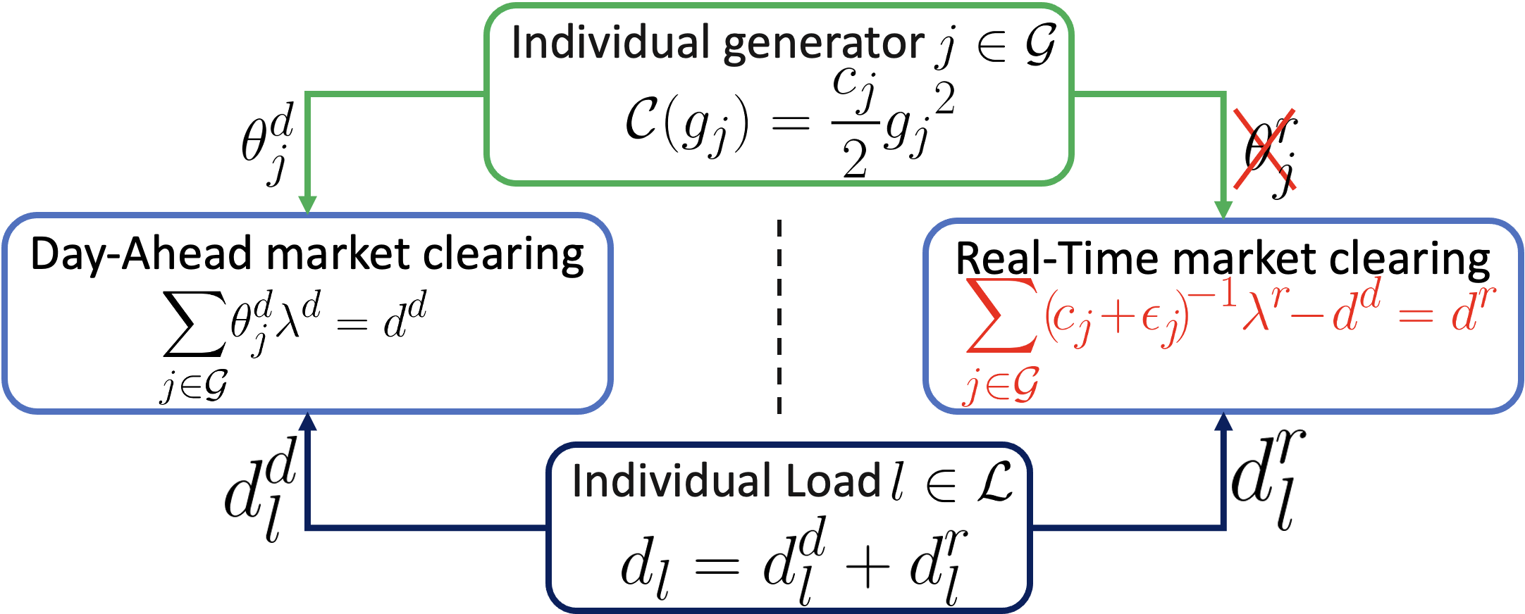
III-B Real-Time MPM Policy

In this section, we first discuss the modified market model, the individual incentives of participants, and then characterize market equilibrium for a real-time MPM policy.

III-B1 Modeling Real-Time MPM Policy

In the case of a real-time MPM policy, the market ignores generators’ bids in real-time, as shown in Figure 2, and roughly estimates the cost of dispatching generator $j$ with an error $\epsilon_{j}\geq 0$ , given the day-ahead dispatch $g_{j}^{d}$

\displaystyle g_{j}^{r}=(c_{j}+\epsilon_{j})^{-1}\lambda^{r}-g_{j}^{d}

(24)

Using the two-stage generation and supply-demand balance (9) and real-time dispatch (24) we get

\displaystyle{\lambda^{r}}=\frac{d}{\sum\limits_{j\in\mathcal{G}}(c_{j}+\epsilon_{j})^{-1}}

(25)

III-B2 Price-taking Participation and Competitive Equilibrium

For the individual incentive problem in a two-stage market with real-time MPM policy, substituting the day-ahead supply function (3), real-time true dispatch condition (24) and real-time clearing prices (25) in (10), we get

\displaystyle\!\!\pi_{j}(\theta_{j}^{d},\!\lambda^{d})\!=

\displaystyle\ \!\theta_{j}^{d}{{\lambda\!}^{d}}^{2}\!\!+\!\frac{d}{\sum\limits_{k\in\mathcal{G}}\!\!c_{k}^{-1}}\!\!\left(\!\omega_{j}d\!-\theta_{j}^{d}{{\lambda\!}^{d}}\!\right)\!\!-\!\frac{c_{j}}{2}\!{\left(\omega_{j}d\right)}^{2}

(26)

where $\omega_{j}:=\frac{(c_{j}+\epsilon_{j})^{-1}}{\sum\nolimits_{k\in\mathcal{G}}(c_{k}+\epsilon_{k})^{-1}}$ . Hence, an individual problem of a price-taking generator is:

\displaystyle\max_{\theta_{j}^{d}}\ \pi_{j}(\theta_{j}^{d};\lambda^{d})

(27)

Similarly, substituting the clearing price (25) in (12) we get,

\displaystyle\rho_{l}(d_{l}^{d},\lambda^{d}):=\lambda^{d}d_{l}^{d}+\frac{d}{\sum_{k\in\mathcal{G}}(c_{k}+\epsilon_{k})^{-1}}(d_{l}-d_{l}^{d})

(28)

such that the individual problem for load $l$ is given by:

\displaystyle\min_{d_{l}^{d}}\

\displaystyle\rho_{l}(d_{l}^{d};\lambda^{d})

(29)

The competition between price-taking participants for individual incentives leads to a set of competitive equilibria, as characterized below.

Theorem 3

The competitive equilibrium in a two-stage market with a real-time MPM policy exists, and given by:


	$\displaystyle g_{j}^{d}+g_{j}^{r}\!=\frac{(c_{j}+\epsilon_{j})^{-1}}{\sum\nolimits_{k\in\mathcal{G}}(c_{k}+\epsilon_{k})^{-1}}d,\ \theta_{j}^{d}\in\mathbb{R}_{\geq 0}\ \forall j\in\mathcal{G}$		(30a)
	$\displaystyle d_{l}^{d}+d_{l}^{r}=d_{l},\ \!\!\forall l\in\mathcal{L}$		(30b)
	$\displaystyle\lambda^{d}=\lambda^{r}=\frac{d}{\sum\nolimits_{k\in\mathcal{G}}(c_{k}+\epsilon_{k})^{-1}}$		(30c)

We provide proof of the theorem in Appendix A. At the competitive equilibrium, the market clearing prices are equal in the two stages, meaning there is no incentive for a load to allocate demand in the day-ahead market, e.g., current market practice. However, the resulting equilibrium in Theorem 3 is inefficient and does not always align with the social planner problem.

Corollary 1

The competitive equilibrium in a two-stage market with a real-time MPM policy (30) also solves the social planner problem (1) only when $\epsilon_{j}=0,\ \forall j\in\mathcal{G}$ ,

III-B3 Price-Anticipating Participation and Nash Equilibrium

The individual problem of each price-anticipating generator $j$ , given by:

\displaystyle\!\!\max_{\theta_{j}^{d},\lambda^{d}}\ \!\pi_{j}\!\left(\theta_{j}^{d},\lambda^{d}\!\left(\theta_{j}^{d};\overline{\theta}_{-j}^{d},d^{d}\right)\right)\ \textrm{ s.t. }\eqref{da_power_bal}

(31)

where generator $j$ maximizes its profit in the two-stage market. The individual problem of price-anticipating load is:

\displaystyle\!\!\!\min_{d_{l}^{d},\lambda^{d}}\ \rho_{l}\!\left(d_{l}^{d},\lambda^{d}\!\left(d_{l}^{d};\theta_{j}^{d},\overline{d}_{-l}^{d}\right)\right)\ \textrm{ s.t. }\eqref{da_power_bal}

(32)

where the load $l$ minimizes its payment in the market.

We study the resulting sequential game where players anticipate each other actions and prices in the market, and the day-ahead clears before the real-time market. To this end, we analyze the game backward, starting from the real-time market, where prices are fixed due to MPM policy (25), followed by the day-ahead market, where participants make decisions for optimal individual incentives and compute the equilibrium path. Generators do not bid in real-time, but loads are allowed to bid in the market. However, load makes decisions simultaneously in the day-ahead market due to inelasticity, fixing their bids in the real-time market, which affects the two-stage market clearing. The following theorem characterizes the two-stage Nash equilibrium that satisfies the Definition (3).

Theorem 4

The Nash equilibrium in a two-stage market with a real-time MPM policy does not exist.

We provide proof of the theorem in Appendix B and a brief insight below into the loss of equilibrium. The price-anticipating participants compete with each other to manipulate prices in the day-ahead given by (4):

\displaystyle\lambda^{d}=\frac{d^{d}}{\sum\limits_{j\in\mathcal{G}}\theta_{j}^{d}}

(33)

while the prices in the real-time $\lambda^{r}$ (25) is fixed. Loads bid decreasing quantities $d_{l}^{d}$ to reduce clearing prices in the day-ahead market and minimize the load payment. Simultaneously, generators bid decreasing parameter $\theta_{j}^{d}$ to increase clearing prices and maximize revenue. The competition between loads and generators for individual incentives in the day-ahead market drives all the demand to the real-time market, where generators operate truthfully. However, in our market mechanism, loads then have the incentive to deviate and allocate demand in the day ahead where prices are zero, meaning zero payment in the market, see Rule 2. Such unilateral load deviations result in deviations from generators to increase clearing prices in the day-ahead market. Therefore the equilibrium does not exist. Without such a market rule, the Nash equilibrium does exist with undefined clearing prices in the day-ahead and all demand allocated to the real-time market. Nevertheless, since day-ahead accounts for a majority of energy trades, the resulting equilibrium is undesirable.

III-C Day-Ahead MPM Policy

In this section, we define the individual incentive of participants and characterize market equilibrium for a day-ahead MPM policy.

III-C1 Modeling Day-Ahead MPM Policy

In the case of a day-ahead MPM policy, as shown in Figure 3, the market ignores the generators’ bids and roughly estimates the cost of dispatching generator $j$ in the day-ahead with an error $\epsilon_{j}\geq 0$ , as given by:

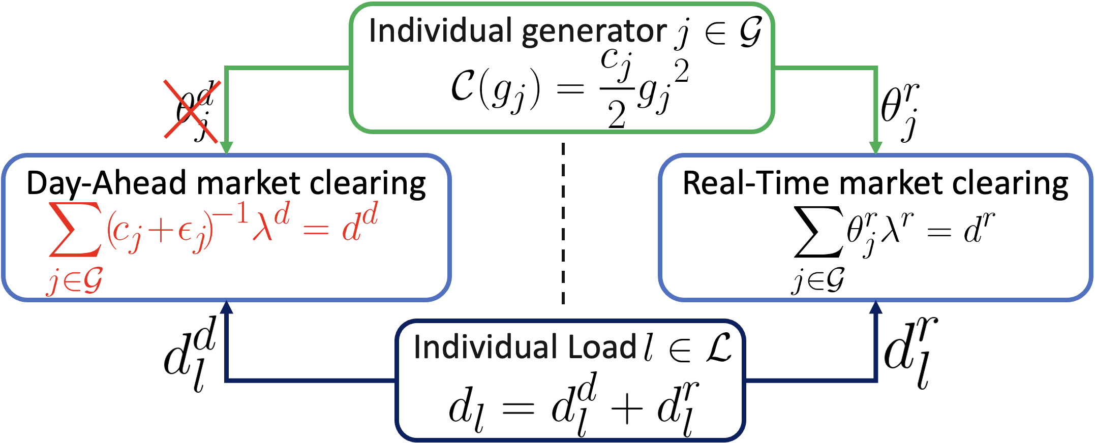
\displaystyle g_{j}^{d}=(c_{j}+\epsilon_{j})^{-1}\lambda^{d}

(34)

Moreover, using day-ahead power balance constraint, we get

\displaystyle\lambda^{d}=\frac{d^{d}}{\sum_{j\in\mathcal{G}}(c_{j}+\epsilon_{j})^{-1}}

(35)

III-C2 Price-taking Participation and Competitive Equilibrium

For the individual incentive problem in a two-stage market with a day-ahead MPM policy, substituting the clearing price (35) in (10), we get

\displaystyle\!\pi_{j}(\theta_{j}^{r};\!\lambda^{r})\!=\!\!(c_{j}\!+\!\epsilon_{j})(\omega_{j}{d^{d}})^{2}\!+\!\theta_{j}^{r}{\lambda^{r}}^{2}\!-\!\frac{c_{j}}{2}\!\!\left(\!\omega_{j}d^{d}\!+\!\theta_{j}^{r}{\lambda^{r}}\!\right)^{2}

(36)

where $\omega_{j}:=\frac{(c_{j}+\epsilon_{j})^{-1}}{\sum\nolimits_{k\in\mathcal{G}}(c_{k}+\epsilon_{k})^{-1}}$ . The individual problem for price-taking generator $j$ is:

\displaystyle\max_{\theta_{j}^{r}}\ \pi_{j}(\theta_{j}^{r};\lambda^{r})

(37)

and the individual problem for load $l$ is given by (12). The resulting competitive equilibrium given the clearing prices $\lambda^{d}$ and $\lambda^{r}$ is characterized below.

Theorem 5

The competitive equilibrium in a two-stage market with a day-ahead MPM policy exists and is given by:


	$\displaystyle\!\!\!g_{j}^{d}=\frac{(c_{j}+\epsilon_{j})^{-1}}{\sum_{j\in\mathcal{G}}c_{j}^{-1}}d,\!\ g_{j}^{r}=\frac{\epsilon_{j}c_{j}^{-1}}{c_{j}\!+\!\epsilon_{j}}\frac{d}{\sum_{j\in\mathcal{G}}c_{j}^{-1}}\ \forall j\in\mathcal{G}$		(38a)
	$\displaystyle\!\!\!d_{l}^{d}\!+\!d_{l}^{r}\!=\!d_{l},\ \!\forall l\in\mathcal{L},\!\ d^{d}\!=\!\frac{\sum\limits_{j\in\mathcal{G}}\!(c_{j}\!+\!\epsilon_{j})^{-1}}{\sum\limits_{j\in\mathcal{G}}c_{j}^{-1}}d,\!\ d^{r}\!=\!d\!-\!d^{d}$		(38b)
	$\displaystyle\!\!\theta_{j}^{r}=\frac{\epsilon_{j}c_{j}^{-1}}{c_{j}\!+\!\epsilon_{j}},\ \lambda^{d}=\lambda^{r}=\frac{1}{\sum_{j\in\mathcal{G}}c_{j}^{-1}}d$		(38c)

We provide proof of the theorem in Appendix C. Unlike the competitive equilibrium for a real-time MPM policy in (30) with equal prices across stages, the loads at equilibrium (38) allocate a majority of the demand in the day-ahead. The incentive for day-ahead demand allocation is a desired market outcome and is not generally satisfied by other market mechanisms. The resulting equilibrium exists as price-taking loads do not anticipate the effect of their bid on the market prices, meaning the payment remains the same for any allocation across the two stages. Moreover, the market outcome (38) solves the social planner problem (1).

III-C3 Price-Anticipating Participation and Nash Equilibrium

The individual problem of each price-anticipating generator $j$ , given by:

\displaystyle\!\!\max_{\theta_{j}^{r},\lambda^{r}}\ \!\pi_{j}\!\left(\theta_{j}^{r},\lambda^{d}\!\left(d^{d}\right),\lambda^{r}\!\!\left(\theta_{j}^{r};\overline{\theta}_{-j}^{r},d^{r}\right)\right)\textrm{ s.t. }\eqref{rt_power_bal}

(39)

where generator $j$ maximizes its profit in the market. The individual problem of price-anticipating load $l$ , is given by:

\displaystyle\!\!\!\min_{d_{l}^{d},\lambda^{r}}\ \rho_{l}\!\left(d_{l}^{d},\lambda^{d}\!\left(d_{l}^{d};\overline{d}_{-l}^{d}\right),\lambda^{r}\!\!\left(d_{l}^{d};\theta_{j}^{r},\overline{d}_{-l}^{r}\right)\right)\textrm{ s.t. }\eqref{rt_power_bal}

(40)

where load $l$ minimizes its payment in the market.

In the market model with a day-ahead MPM policy, generators make decisions in real-time while load can make decisions in the day-ahead. The resulting two-stage sequential game is essentially a leader-follower Stackelberg-Nash game, where generators are followers in the real-time market and loads are leaders in the day-ahead market, and each participant in their respective groups competes amongst themselves in a Nash game. We follow the terminology used in [27] to describe similar formulations in different markets. For the closed form solution, we assume that generators are homogeneous in the sense that they share the same cost coefficient, i.e. $c_{j}=:c,\ \forall j\in\mathcal{G}$ and bid symmetrically in the market, i.e. $\theta_{j}^{r}=:\theta^{r},\ \forall j\in\mathcal{G}$ . Under these assumptions, the Nash equilibrium is characterized below.

Theorem 6

Assume that generators are homogeneous and bid symmetrically in the market. Also, assume that estimation error is same for homogeneous generators, i.e. $\epsilon_{j}:=\epsilon,\ \forall j\in\mathcal{G}$ . If more than two generators are participating in the market i.e., $G\geq 3$ and the number of individual loads participating in the market satisfies $\frac{1}{L}>\frac{c-\epsilon(G-2)}{(c+\epsilon)(G-2)}$ , then the symmetric Nash equilibrium in a two-stage market with a day-ahead MPM policy exists uniquely as:


	$\displaystyle\!\!\!g_{j}^{d}\!=\!\frac{c}{c\!+\!\epsilon}\frac{L}{L\!+\!1}\frac{G\!-\!1}{G\!-\!2}\frac{d}{G},\!\ g_{j}^{r}\!\!=\!\!\left(\!1\!-\!\frac{c}{c\!+\!\epsilon}\frac{L}{L\!+\!1}\frac{G\!-\!1}{G\!-\!2}\!\right)\frac{d}{G}$		(41a)
	$\displaystyle\!\!\!d_{l}^{d}\!=\!\frac{c}{c\!+\!\epsilon}\frac{1}{L\!+\!1}\frac{G\!-\!1}{G\!-\!2}d,\!\ d_{l}^{r}\!\!=\!\!\left(\!\!d_{l}\!-\!\frac{c}{c\!+\!\epsilon}\frac{1}{L\!+\!1}\frac{G\!-\!1}{G\!-\!2}d\right)$		(41b)
	$\displaystyle\theta^{r}\!=\!\frac{1}{c}\left(\frac{G\!-\!2}{G\!-\!1}\!-\!\frac{c}{c\!+\!\epsilon}\frac{L}{L\!+\!1}\right)$		(41c)
	$\displaystyle\lambda^{d}=\frac{L}{L\!+\!1}\frac{G\!-\!1}{G\!-\!2}\frac{c}{G}d,\ \lambda^{r}=\frac{G\!-\!1}{G\!-\!2}\frac{c}{G}d.$		(41d)

Moreover, for $\frac{1}{L}\leq\frac{c-\epsilon(G-2)}{(c+\epsilon)(G-2)}$ , a symmetric equilibrium does not exist.

We provide proof of the Theorem in Appendix D. Unlike the market with a real-time MPM policy, the Nash equilibrium exists in the market with a day-ahead MPM policy. However, it requires restrictive conditions on the number of participants in the market and may not even exist in other cases. We discuss these cases with no symmetric Nash equilibrium and provide intuition into participants’ behavior in the market:

1

$\mathbf{\frac{1}{L}<\frac{c-\epsilon(G-2)}{(c+\epsilon)(G-2)}}:$ In this case, the net demand is negative in the real-time market. The first order condition implies that each generator $j$ acts as load, paying $\lambda^{r}g_{j}^{r}$ as part of the market settlement since their optimal bid $\theta_{j}^{r}<0$ and the real-time clearing price $\lambda^{r}>0$ . However, if the generators bid $\theta_{j}^{r}>0$ , then the linear supply function implies that each generator $j$ dispatch $g_{j}^{r}<0$ at the clearing prices $\lambda^{r}<0$ earning revenue in the market. However, this is not desirable from a load perspective since they are making payments in the market and they have the incentive to deviate to minimize their payment. Hence, symmetric equilibrium with negative demand in the real-time market does not exist as the symmetric bid $\theta_{j}^{r}>0$ does not satisfy the first-order condition. The dependence of the individual bid $\theta_{j}^{r}$ on the given bids from other participants makes the closed-form analysis challenging, and any guarantee of the existence of equilibrium is hard.
2

$\mathbf{\frac{1}{L}=\frac{c-\epsilon(G-2)}{(c+\epsilon)(G-2)}}:$ In this case, no symmetric Nash equilibrium exists. Loads take advantage of the truthful participation of generators in day-ahead market and their ability to anticipate impact of bids on the clearing prices. Regardless of generators’ bids, loads have the incentive to deviate by allocating demand in the real-time market with a lower clearing price.

Corollary 2

For ${\frac{1}{L}>\frac{c-\epsilon(G-2)}{(c+\epsilon)(G-2)}}$ , at the Nash equilibrium (41) in a two-stage market with a day-ahead MPM policy, the demand allocation is given by:


	$\displaystyle\sum_{l\in\mathcal{L}}d_{l}^{d}=d^{d}=\frac{c}{c+\epsilon}\frac{L}{L+1}\frac{G-1}{G-2}d$		(42a)
	$\displaystyle\sum_{l\in\mathcal{L}}d_{l}^{r}=d^{r}=\left(1-\frac{c}{c+\epsilon}\frac{L}{L+1}\frac{G-1}{G-2}d\right)d$		(42b)

Assuming $\epsilon=0$ , the following relation holds,

d^{d}\in(0.5d,d),\ d^{r}\in(0,0.5d)

IV Equilibrium Analysis

In this section, we study the properties of market equilibrium under the proposed policy framework and compare it with the standard market equilibrium.

IV-A Comparison of a stage-wise MPM Policy

An MPM policy in real-time either results in an inefficient market outcome at the competitive equilibrium or leads to no Nash equilibrium. However, an MPM policy in the day-ahead leads to a stable market outcome that is robust to price manipulations, e.g. see Nash equilibrium (41). Despite errors in cost estimations, the competitive equilibrium is efficient (38). This is summarized in Table I.

We further analyze the case of a day-ahead MPM policy to study the strategic behavior of participants while regarding the respective competitive equilibrium in Theorem 5 as a benchmark. In the case of a day-ahead MPM policy, loads act as leaders in the day-ahead and generators as followers in real-time. The generator bids to manipulate prices leading to inflated prices in real-time (41d) while the load shifts its allocation in the day-ahead (41b), increasing prices in the day-ahead market. Though the market equilibrium deviates from the competitive equilibrium (38), the social cost remains the same due to the homogeneous participation of generators. Table II summarizes the aggregate profit and aggregate payment of generators and loads, respectively.

TABLE I: Competitive Equilibrium (CE) and Nash Equilibrium (NE) with a stage-wise MPM policy

Instance	Real-Time MPM	Day-Ahead MPM
CE	Non-unique equilibrium	Unique equilibrium
	Do not achieve social cost	Achieve social cost
	Arbitrary demand allocation	Higher demand in day-ahead
NE	Does not exist	Symmetric equilibrium
	-	Social Cost same as CE
	-	Extra constraints on players

Corollary 3

For $L<G-2$ , the aggregate payment of loads and aggregate profit of generators at symmetric Nash equilibrium (41) is less than that at respective competitive equilibrium (38). Moreover, for $L\geq G-2$ and ${\frac{1}{L}>\frac{c-\epsilon(G-2)}{(c+\epsilon)(G-2)}}$ , the aggregate payment of loads and aggregate profit of generators at symmetric Nash equilibrium (41) is greater than that at respective competitive equilibrium (38).

The corollary follows from comparing the aggregate profit (payment) at Nash equilibrium to that at competitive equilibrium in Table II for $L<G-2$ .

IV-B Equilibrium comparison with a standard market

In this section, we compare the equilibrium in a day-ahead MPM policy market to a standard market. The social cost at the competitive equilibrium remains the same for the two markets with equal prices in the two stages. However, unlike in the case of a day-ahead MPM policy, the competitive equilibrium in Theorem 1 exists non-uniquely and there is no incentive for a load to allocate demand in the day-ahead market.

Interestingly, at Nash equilibrium prices in the two stages are the same for a day-ahead MPM policy market (41d) and a standard market (22). Furthermore, an error in the estimation of the cost of dispatching generators does not impact market prices due to the participation of homogeneous generators. However, the dispatch of generators and allocation of demand is different in the two market settings due to a leader-follower structure between participants in the market with a day-ahead MPM policy. To understand the impact of price-anticipating participants on market equilibrium, we compare the aggregate profit (payment) in Table II and III, respectively.

TABLE II: Comparison between Competitive Equilibrium (CE) and Nash Equilibrium (NE) in a market with a day-ahead MPM policy

Case	Generators total profit	Loads total payment
CE	$\frac{1}{2}\frac{c}{G}d^{2}$	$\frac{c}{G}d^{2}$
NE	$\frac{1}{2}\!\frac{c}{G}d^{2}\!\!\left(\!\frac{G}{G-2}\!-\!\frac{c}{c+\epsilon}\frac{(G-1)^{2}}{(G-2)^{2}}\frac{2L}{(L+1)^{2}}\!\!\right)$	$\frac{c}{G}d^{2}\!\!\left(\!\frac{G-1}{G-2}\!-\!\frac{c}{c+\epsilon}\frac{(G-1)^{2}}{(G-2)^{2}}\frac{L}{(L+1)^{2}}\!\!\right)$

TABLE III: Comparison between Competitive Equilibrium (CE) and Nash Equilibrium (NE) in a standard market

Case	Generators total profit	Loads total payment
CE	$\frac{1}{2}\frac{c}{G}d^{2}$	$\frac{c}{G}d^{2}$
NE	$\frac{1}{2}\!\frac{c}{G}d^{2}\!\!\left(\!\frac{G}{G-2}\!-\!\frac{2L(G-1)+2}{(L+1)^{2}(G-2)}\!\right)$	$\frac{c}{G}d^{2}\!\!\left(\!\frac{G-1}{G-2}\!-\!\frac{L(G-1)+1}{(L+1)^{2}(G-2)}\!\right)$

We restrict our comparison for $\frac{1}{L}>\frac{c-\epsilon(G-2)}{(c+\epsilon)(G-2)}$ only since the Nash equilibrium in Theorem 6 does not exist otherwise. In particular, for $L=G-3$ the aggregate profit (payment) as shown in row 2 of Table III at the Nash equilibrium in Theorem 2 equals to that of the competitive equilibrium. However, for $L<G-3$ the aggregate profit (payment) at Nash equilibrium is always less than the competitive equilibrium, meaning the loads are winners. The change in the normalized aggregate profit (payment) at the Nash equilibrium between a market with a day-ahead MPM policy and a standard market is given by

\frac{2}{(L+1)^{2}}\frac{1}{G-2}\left(1-\frac{L}{G-2}-L+\frac{\epsilon}{c+\epsilon}L(G-1)\right)

where profit (payment) is normalized with the competitive equilibrium. The difference depends on the number of participants and as the number of participants increases, the difference tends to $0$ , since the Nash equilibrium in both cases approaches the competitive equilibrium, respectively.

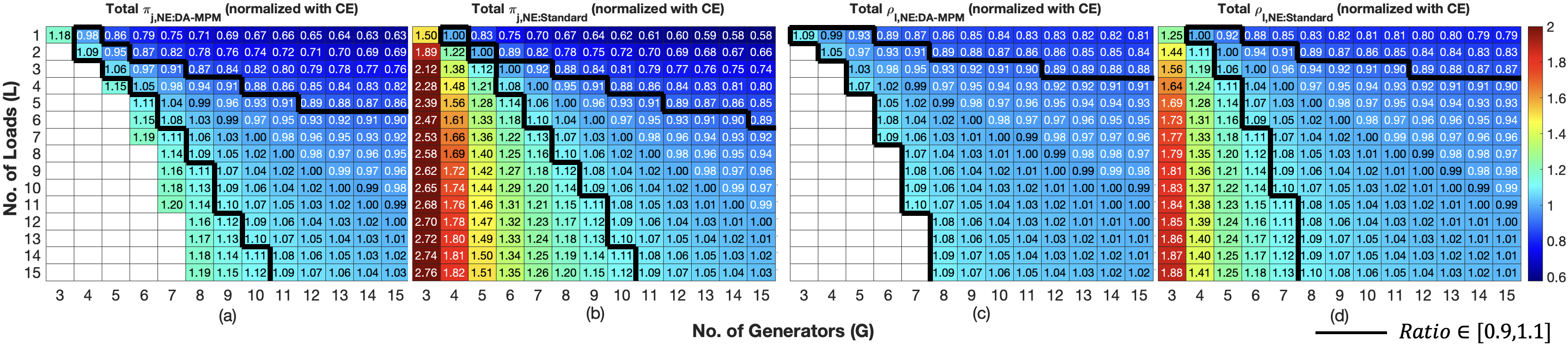
Figure 4 compares the total profit (payment) normalized with competitive equilibrium for a day-ahead MPM (DA-MPM) policy market and a standard market for cost estimation error $\epsilon=0.1$ , respectively, as we change the number of loads ( $l\in\mathcal{L},\ L\in\{1,\ldots,G-3\}$ ), and generators ( $j\in\mathcal{G},\ G\in\{4,\ldots,20\}$ ). The ratio decreases monotonically as the number of generators increases, meaning the increased competition between more generators to meet the inelastic demand gives more power to loads, allowing them to reduce their payment even further, as shown by the horizontal rows in all panels in Figure 4. Furthermore, the ratio increases monotonically as the number of loads increases (for a large enough number of generators), meaning the market power shifts between loads and generators, as shown by the vertical color columns in panels (a) and (b) in Figure 4. In particular, in both markets, we observe a reversal in power, e.g., for a large number of loads generators make a higher profit at the expense of loads in the market and vice versa, as shown in panels (b) and (d) in the Figure 4.

Additionally, implementing the day-ahead MPM policy helps reduce market power. This leads to a total profit (payment) at Nash equilibrium that is closer to competitive equilibrium levels than what is observed in standard markets, as demonstrated in panels (a) and (c) for profit and panels (b) and (d) for payment in Figure 4. Unfortunately, with a day-ahead MPM policy, the equilibrium does not always exists as shown by white-colored cells in panels (a) and (c). Finally, in the limit $L\rightarrow\infty\implies G\rightarrow\infty$ , the Nash equilibrium converges to competitive equilibrium, also shown in Table II.

V Numerical Study

We now investigate how the cost estimation error, heterogeneity in cost coefficients, and load size affect individual incentives at Nash equilibrium in the market with a day-ahead MPM. We overcome the theoretical complexity of the closed-form analysis and run numerical best-response studies to understand the impact on market equilibrium. To this end, we consider the case of 2 price-anticipating loads and 5 price-anticipating generators in a two-stage market.

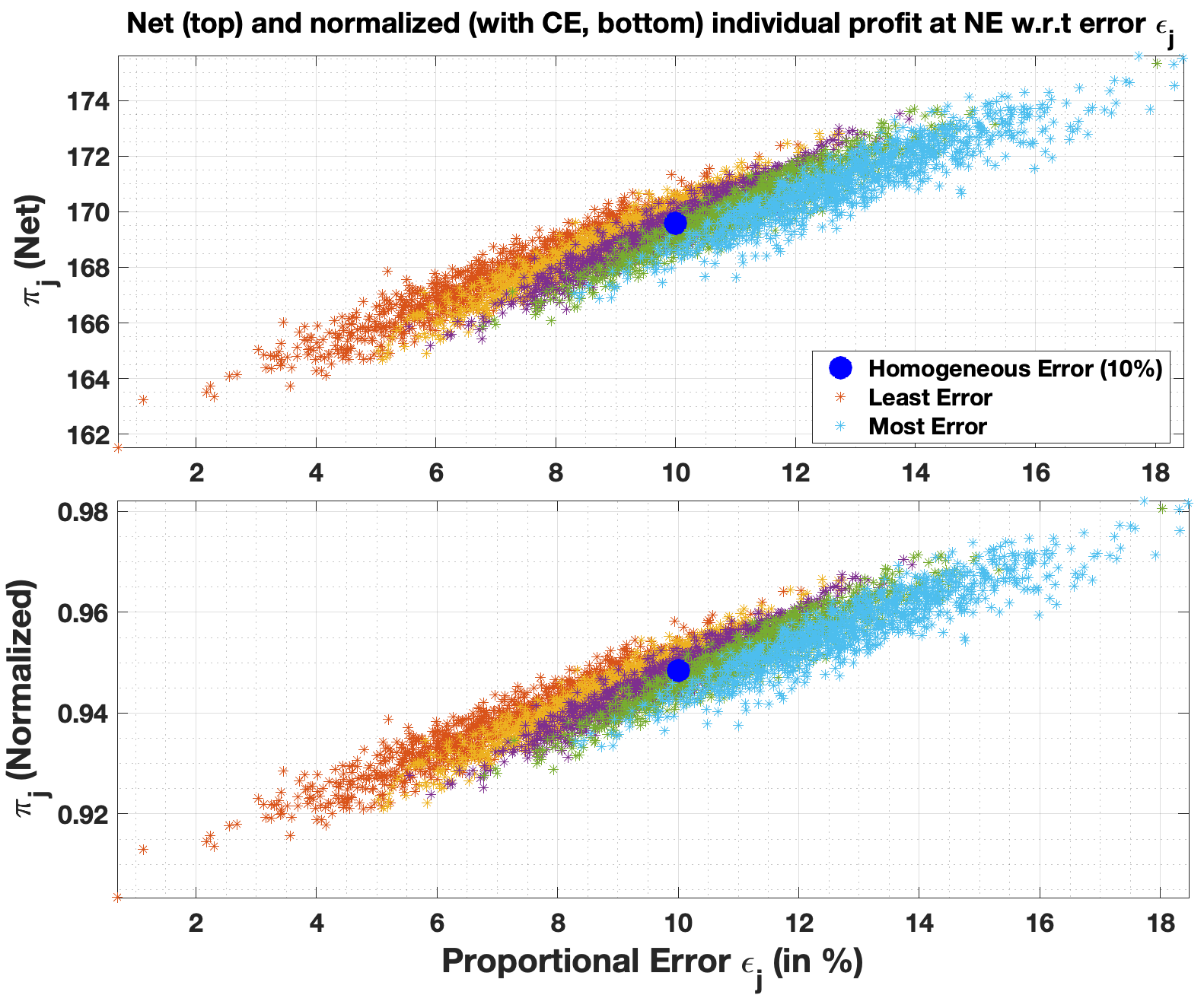
The individual aggregate inelastic load is given by $d_{l}=[99.4,199.6]^{T}\ MW$ from the Pennsylvania, New Jersey, and Maryland (PJM) data miner day-ahead demand bids [28]. For each generator $j$ with a truthful cost coefficient $c_{j}=0.1\$/MW^{2},\ \forall j\in\mathcal{G}$ corresponding to the cost coefficients from the IEEE 300-bus system [29]. We assume a proportional error $\epsilon_{j}=\delta_{j}c_{j}$ such that estimated cost coefficient is given by $\hat{c}_{j}=c_{j}(1+\delta_{j}),\ \forall j\in\mathcal{G}$ . The cost estimation error of generators are sampled $10,000$ times from a Gaussian distribution with mean $10\%$ and variance $2.5\%$ , i.e. $\delta_{j}\sim N(0.1,0.025)\ \forall j\in\{1,...,5\}$ . The top and bottom panel in Figure 5 plots the net profit and the normalized profit (normalized with the competitive equilibrium) at Nash equilibrium, respectively. An increase in estimation error results in a higher net profit at Nash equilibrium, as shown in the top panel in Figure 5. Furthermore, errors in cost estimation also mitigate the market power of loads with profits closer to the competitive one.

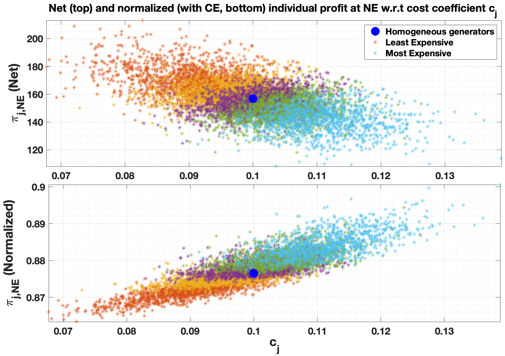
We next analyze the impact of heterogeneity in cost coefficients on market equilibrium. For ease of exposition, we assume that the cost estimation error $\epsilon_{j}=0\ \forall j\in\{1,...,5\}$ . Our analysis is focused on capturing the qualitative impact of heterogeneity in cost coefficients on system-level market power. To this end, we choose a Gaussian distribution to model the uncertainty in the market operator’s estimate for generators’ truthful cost as the first step toward understanding the potential impact. The cost coefficients of generators are sampled $10,000$ times from a Gaussian distribution with mean $0.1$ and sample variance $0.001$ for a sample of cost coefficients from the IEEE 300-bus system [29], i.e. $c_{j}\sim N(0.1,0.001),\ \forall j\in\{1,...,5\}$ . The top and bottom panel in Figure 6 plots the absolute profit and the normalized profit (normalized with the competitive equilibrium) at Nash equilibrium, respectively. The cheaper generators earn a higher profit when compared with the expensive generators with higher cost coefficients at Nash equilibrium. However, the normalized profit ratio in the bottom panel shows that expensive generators have a higher value than cheaper ones, meaning that though expensive generators have lower absolute profit, these are the least exploited in the market. We hypothesize that such a non-trivial behavior is related to the nature of competition between strategic generators instead of an effect of a day-ahead MPM policy. We admit that a closed-form analysis is theoretically complex, and we do not have a thorough mechanism to validate our hypothesis.

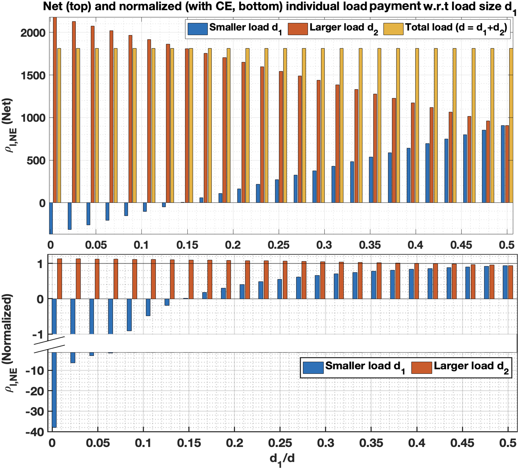
In Figure 7 we show the absolute (top panel) and normalized (bottom panel) load payment w.r.t smaller load size. For this, we keep the same number of loads and generators in the market with varying load sizes for fixed net demand. We again sample cost coefficients from Gaussian distribution with mean $0.1$ and sample variance $0.001$ for a sample of cost coefficients from the IEEE 300-bus system [29], i.e. $c_{j}\sim N(0.1,0.001),\ \forall j\in\{1,...,5\}$ . The cost estimation error $\epsilon_{j}=0,\ \forall j\in\{1,...,5\}$ . The top panel shows that though the net load payment remains the same as we change the size of the load, the smaller load may even make a profit in the market at the expense of a higher load. More formally to develop intuition, in the case of homogeneous generators, the normalized payment ratio for individual load at Nash equilibrium in Theorem 6, is given by

\frac{G-1}{G-2}\left(1-\frac{1}{(L+1)^{2}}\frac{G-1}{G-2}\frac{d}{d_{l}}\right)

which is negative for a sufficiently small load. In particular, the smaller load has a negative normalized ratio at the expense of a higher load (a ratio greater than 1), as shown in the bottom panel of Figure 7. The larger load makes more payment at Nash equilibrium than at the competitive equilibrium, while the aggregate payment of the set of loads is still less than at the competitive equilibrium. Though the heterogeneity in load size does not affect the net payment or the group behavior in the market, a smaller load makes negative payments at the expense of larger loads and can exercise more market power.

VI Discussions

In this section, we discuss the limitations of the study and potential implications for policymakers.

VI-A Limitations of the study

The closed-form analysis of supply function equilibrium in a two-stage settlement market is theoretically complex and the system is often analyzed under certain simplifying market assumptions. While there are works that certainly consider a more relaxed set of assumptions, they either study single-stage market [25, 12, 19, 18], competitive market structure [22, 17, 18], inelastic demand [30, 31], homogeneous participants or symmetric participation [1, 32], etc. Given that the supply-function Nash equilibria are generally hard to characterize, even for a single-stage market, the literature often uses this approach as a zero-order analysis [1, 32]. We further note that our findings are consistent with the theory in our numerical experiments, where we relax, for e.g., the homogeneity constraints. Although capacity constraints, network constraints, etc., impact market power, our focus is on system-level market power, which occurs regardless of these constraints. Furthermore, an analysis contemplating all of such settings, though interesting, will be too nuanced and digressed from our goal of counterfactual study.

VI-B Implications for policymakers

Our work highlights the importance of counterfactual analysis of two specific system-level policies in the CAISO area. Despite the CAISO’s proposal of implementing a real-time MPM policy in the first phase, it should not be deployed by itself. We show that such a policy results in an inefficient competitive equilibrium, while the Nash equilibrium does not exist. We believe that if a strategy does not work well in a simple setting, then is unlikely to do well in a more complicated one. A day-ahead policy seems to have a reasonable impact on the market outcome that merits further analysis (with capacity constraints, network constraints, etc.) and consideration. Despite errors in cost estimations of generators, it results in an efficient competitive equilibrium, meaning the outcome aligns with the social planner problem. Moreover, the Nash equilibrium is more robust to market power and price manipulations. The aggregate profit (payment) of participants at Nash equilibrium is comparatively closer to the competitive one. Furthermore, the impact of error in cost estimation, heterogeneity in cost coefficient, and diversity in load size help policymakers with the tools to ensure fairness in the market. A positive bias in estimation leads to more profits for generators and mitigation of market power of loads. Larger loads may tend to split into smaller loads that merit further analysis to ensure market fairness.

VII Conclusions

We study competition between generators (bid linear supply function) and loads (bid quantity) in a two-stage settlement electricity market with a stage-wise MPM policy. In the proposed policy framework, CAISO substitutes generator bids with default bids in the stage with an MPM policy, i.e., day-ahead or real-time. To understand the participant behavior in the market, we start with a real-time MPM policy and analyze the sequential game, where generators only bid in the day-ahead market. The resulting competitive equilibrium, price-taker participants, is inefficient, while the Nash equilibrium, price-anticipating participants, does not exist, indicating an unstable market outcome.

Despite the estimation error, in the case of a day-ahead MPM policy, the competitive equilibrium aligns with the social planner problem. Further, the Nash equilibrium is robust to price manipulations compared to the standard market. Notably, our analysis shows that demand, despite being inelastic, could shift its allocation to manipulate market prices and win the competition. A more nuanced analysis of cost estimation error and heterogeneity in cost coefficients benefits generator over loads. In the case of heterogeneous generators, expensive generators are less affected in the market. Also, the load size diversity highlights the role of a sufficiently smaller load in exercising market power at the expense of larger loads.

References

[1] P. You, M. A. Fernandez, D. F. Gayme, and E. Mallada, “The role of strategic participants in two-stage settlement markets,” Technical Report, 2022. [Online]. Available: https://pengcheng-you.github.io/desires-lab/papers/YFGM_OR_TR.pdf
[2] R. K. Bansal, Y. Chen, P. You, and E. Mallada, “Equilibrium analysis of electricity markets with day-ahead market power mitigation and real-time intercept bidding,” in Proceedings of the Thirteenth ACM International Conference on Future Energy Systems, ser. e-Energy ’22. New York, NY, USA: Association for Computing Machinery, 2022, p. 47–62. [Online]. Available: https://doi.org/10.1145/3538637.3538839
[3] Y. Xu and S. H. Low, “An efficient and incentive compatible mechanism for wholesale electricity markets,” IEEE Transactions on Smart Grid, vol. 8, no. 1, pp. 128–138, 2017.
[4] S. Borenstein, J. Bushnell, C. Knittel, and C. Wolfram, “Inefficiencies and market power in financial arbitrage: a study of california’s electricity markets,” Journal of Industrial Economics, vol. 56, pp. 347–378, 06 2008.
[5] C. Graf, E. L. Pera, F. Quaglia, and F. Wolak, “Market power mitigation mechanisms for wholesale electricity markets: Status quo and challenges,” The Freeman Spogli Institute for International Studies, Stanford, Technical Report, Jun 2021. [Online]. Available: https://web.stanford.edu/group/fwolak/cgi-bin/sites/default/files/MPM_Review_GPQW.pdf
[6] “Day-ahead market enhancements, second revised straw proposal,” California Independent System Operator, Tech. Rep., July 2021.
[7] P. Servedio, “California independent system operator corporation scoping document - system market power mitigation,” California Independent System Operator, Tech. Rep., Sept 2019, accessed April 2022. [Online]. Available: https://www.caiso.com/Documents/ScopingDocument-SystemMarketPowerMitigation.pdf
[8] P. Servedio, D. Tavel, and D. Johnson, “System market power mitigation, draft final proposal,” California Independent System Operator, Tech. Rep., Jun 2020.
[9] “California independent system operator corporation extended day-ahead market straw proposal - bundle one,” California Independent System Operator, Tech. Rep., July 2020, accessed April 2022. [Online]. Available: https://www.caiso.com/InitiativeDocuments/StrawProposal-ExtendedDay-AheadMarket-BundleOneTopics.pdf
[10] “California independent system operator corporation fifth replacement ferc electric tariff,” California Independent System Operator, Tech. Rep. Section 30, Sept 2022. [Online]. Available: http://www.caiso.com/Documents/Conformed-Tariff-as-of-Sep1-2022.pdf
[11] “California independent system operator corporation decision on commitment costs and default energy bid enhancements proposal,” California Independent System Operator, Tech. Rep., March 2018. [Online]. Available: https://www.caiso.com/Documents/Decision_CCDEBEProposal-Memo-Mar2018.pdf
[12] R. Johari, “Efficiency loss in market mechanisms for resource allocation,” Ph.D. dissertation, Massachusetts Institute of Technology, 2004. [Online]. Available: http://hdl.handle.net/1721.1/16694
[13] H. Mohsenian-Rad, “Optimal demand bidding for time-shiftable loads,” IEEE Transactions on Power Systems, vol. 30, no. 2, pp. 939–951, 2015.
[14] X. Lin, B. Wang, Z. Xiang, and Y. Zheng, “A review of market power-mitigation mechanisms in electricity markets,” Energy Conversion and Economics, vol. 3, no. 5, pp. 304–318, 2022.
[15] A. Kumar David and F. Wen, “Market power in electricity supply,” IEEE Transactions on Energy Conversion, vol. 16, no. 4, pp. 352–360, 2001.
[16] L. Marshall, A. Bruce, and I. MacGill, “Assessing wholesale competition in the australian national electricity market,” Energy Policy, vol. 149, p. 112066, 2021. [Online]. Available: https://www.sciencedirect.com/science/article/pii/S0301421520307771
[17] T. Boomsma, S. Pineda, and D. Heide-Jørgensen, “The spot and balancing markets for electricity: open- and closed-loop equilibrium models,” Computational Management Science, vol. 19, 06 2022.
[18] R. K. Bansal, P. You, D. F. Gayme, and E. Mallada, “A market mechanism for truthful bidding with energy storage,” 2021.
[19] Y. Chen, C. Zhao, S. H. Low, and A. Wierman, “An energy sharing mechanism considering network constraints and market power limitation,” IEEE Transactions on Smart Grid, pp. 1–1, 2022.
[20] A. Zerrahn and D. Huppmann, “Network expansion to mitigate market power: How increased integration fosters welfare,” SSRN Electronic Journal, 01 2014.
[21] H. Guo, Q. Chen, Q. Xia, and C. Kang, “Market power mitigation clearing mechanism based on constrained bidding capacities,” IEEE Transactions on Power Systems, vol. 34, no. 6, pp. 4817–4827, 2019.
[22] Y. Ye, D. Papadaskalopoulos, and G. Strbac, “Investigating the ability of demand shifting to mitigate electricity producers’ market power,” IEEE Transactions on Power Systems, vol. 33, no. 4, pp. 3800–3811, 2018.
[23] D. Cai, A. Agarwal, and A. Wierman, “On the inefficiency of forward markets in leader-follower competition,” Operations Research, vol. 68, 06 2016.
[24] Y. Sun, Z. Wang, G. Wang, and B. Wang, “Research on the effects of the most used market power mitigation mechanisms considering different market environments,” Energy Engineering, vol. 119, no. 6, pp. 2193–2210, 2022. [Online]. Available: http://www.techscience.com/energy/v119n6/49698
[25] N. Li, L. Chen, and M. A. Dahleh, “Demand response using linear supply function bidding,” IEEE Transactions on Smart Grid, vol. 6, no. 4, pp. 1827–1838, 2015.
[26] R. Baldick, R. Grant, and E. Kahn, “Theory and application of linear supply function equilibrium in electricity markets,” Journal of Regulatory Economics, vol. 25, pp. 143–167, 03 2004.
[27] M. Li, J. Qin, N. M. Freris, and D. W. C. Ho, “Multiplayer stackelberg-nash game for nonlinear system via value iteration-based integral reinforcement learning,” IEEE Transactions on Neural Networks and Learning Systems, pp. 1–12, 2020.
[28] “Pennsylvania, New Jersey, and Maryland (PJM) data miner,” Available at url, Jun. 2021. [Online]. Available: https://dataminer2.pjm.com/feed/hrl_da_demand_bids/definition
[29] R. D. Zimmerman and C. E. Murillo-Sanchez, “Matpower (version 7.0) [software].” Available at, 2019. [Online]. Available: https://matpower.org/
[30] R. Johari and J. N. Tsitsiklis, “Parameterized supply function bidding: Equilibrium and efficiency,” Operations research, vol. 59, no. 5, pp. 1079–1089, 2011.
[31] P. Holmberg, “Supply function equilibrium with asymmetric capacities and constant marginal costs,” The Energy Journal, vol. 28, no. 2, 2007.
[32] P. D. Klemperer and M. A. Meyer, “Supply function equilibria in oligopoly under uncertainty,” Econometrica, vol. 57, no. 6, pp. 1243–1277, 1989. [Online]. Available: http://www.jstor.org/stable/1913707

Appendix A Proof of Theorem 3

Under price-taking behavior, the individual problem for loads (29) is a linear program with the closed-form solution given by:

\displaystyle\!\!\!\!\left\{\begin{array}[]{l}\!d_{l}^{d}\!=\!\infty,d_{l}^{r}\!=\!-\infty,d_{l}^{d}+d_{l}^{r}\!=\!d_{l},\!\mbox{if }\lambda^{d}\!<\!\frac{d}{\sum\limits_{k\in\mathcal{G}}\!(c_{k}+\epsilon_{k})^{-1}}\\ \!d_{l}^{d}\!=\!-\infty,d_{l}^{r}\!=\!\infty,d_{l}^{d}+d_{l}^{r}\!=\!d_{l},\mbox{if }\lambda^{d}\!>\!\frac{d}{\sum\limits_{k\in\mathcal{G}}\!(c_{k}+\epsilon_{k})^{-1}}\\ \!d_{l}^{d}+d_{l}^{r}=d_{l},\quad\mbox{ if }\lambda^{d}=\frac{d}{\sum\limits_{k\in\mathcal{G}}\!(c_{k}+\epsilon_{k})^{-1}}\end{array}\right.

(46)

where loads prefer the lower price in the market. The individual problem for generators (27) requires:

\displaystyle\left\{\begin{array}[]{l}\theta_{j}^{d}=-\infty,\!\mbox{ if }0\leq\lambda^{d}<\frac{d}{\sum\limits_{k\in\mathcal{G}}\!(c_{k}+\epsilon_{k})^{-1}}\\ \theta_{j}^{d}=\infty,\!\mbox{ if }\lambda^{d}<\frac{d}{\sum\limits_{k\in\mathcal{G}}\!(c_{k}+\epsilon_{k})^{-1}},\textrm{ and }\lambda^{d}<0\\ \theta_{j}^{d}=\infty,\mbox{ if }\lambda^{d}>\frac{d}{\sum\limits_{k\in\mathcal{G}}\!(c_{k}+\epsilon_{k})^{-1}}\\ \theta_{j}^{d}\in\mathbb{R}_{\geq 0},\quad\mbox{ if }\lambda^{d}=\frac{d}{\sum\limits_{k\in\mathcal{G}}\!(c_{k}+\epsilon_{k})^{-1}}\end{array}\right.

(51)

where generators prefer higher prices in the market and seek to maximize profit. At the competitive equilibrium the day-ahead supply function (3), real-time true dispatch condition (24), real-time clearing prices (25), and the individual optimal solution (46),(51) holds simultaneously and this is only possible if the market price is equal in the two-stages, i.e.,

\lambda^{d}=\lambda^{r}=\frac{d}{\sum\limits_{k\in\mathcal{G}}\!(c_{k}+\epsilon_{k})^{-1}},\textrm{s.t }d_{l}=d_{l}^{d}+d_{l}^{r}

From real-time true dispatch conditions we have

g_{j}^{r}+g_{j}^{d}=\frac{(c_{j}+\epsilon_{j})^{-1}d}{\sum\limits_{k\in\mathcal{G}}\!(c_{k}+\epsilon_{k})^{-1}}

Thus a set of competitive equilibria exists.

Appendix B Proof of Theorem 4

From the day-ahead market clearing we have

\displaystyle\sum_{j\in\mathcal{G}}\theta_{j}^{d}\lambda^{d}=d^{d}\implies\lambda^{d}=\frac{1}{\sum_{j\in\mathcal{G}}\theta_{j}^{d}}d^{d}

(52)

where we assume that $\sum_{j\in\mathcal{G}}\theta_{j}^{d}\neq 0$ . Substituting (52) in generator individual profit optimization (31), we get the individual problem of strategic generator $j$ as (we assume that $d^{d}\neq 0$ and leave the discussion of $d^{d}=0$ for later):

	$\displaystyle\!\!\!\max_{\theta_{j}^{d}}$	$\displaystyle\left(\!\frac{d^{d}}{\sum\limits_{k\in\mathcal{G}}\theta_{k}^{d}}\!-\!\frac{d}{\sum\limits_{k\in\mathcal{G}}(c_{k}+\epsilon_{k})^{-1}}\!\right)\!\frac{\theta_{j}^{d}d^{d}}{\sum\limits_{k\in\mathcal{G}}\theta_{k}^{d}}\!$
		$\displaystyle\quad\quad\quad\quad\quad\quad\quad+\!\frac{\frac{c_{j}}{2}+\epsilon_{j}}{(c_{j}+\epsilon_{j})^{2}}\!\!\left(\!\frac{d}{\sum\limits_{k\in\mathcal{G}}(c_{k}+\epsilon_{k})^{-1}}\!\!\right)^{2}$		(53)

Though the individual problem is not necessarily concave in the domain, we can analyze the optimal bidding behavior from the first-order and second-order conditions. Writing the first-order condition, we have

	$\displaystyle\frac{d\pi_{j}}{d\theta_{j}^{d}}=\!\!\left[\!\frac{\theta_{j}^{d}}{\sum\limits_{k\in\mathcal{G}}\theta_{k}^{d}}\!\left(\frac{d}{\sum\limits_{k\in\mathcal{G}}(c_{k}+\epsilon_{k})^{-1}}\!-\!\frac{2d^{d}}{\sum\limits_{k\in\mathcal{G}}\theta_{k}^{d}}\right)\!\!\right.$
	$\displaystyle\quad\quad\quad\quad\quad\quad\left.+\!\!\left(\!\frac{d^{d}}{\sum\limits_{k\in\mathcal{G}}\theta_{k}^{d}}\!-\!\frac{d}{\sum\limits_{k\in\mathcal{G}}(c_{k}+\epsilon_{k})^{-1}}\!\right)\!\!\right]\frac{d^{d}}{\sum\limits_{k\in\mathcal{G}}\theta_{k}^{d}}$		(54)

Now summing over $j\in\mathcal{G}$ to attain the turning point of (54), we have

\displaystyle\implies

\displaystyle(G-2)(d^{d})^{2}-(G-1)\frac{\sum_{j\in\mathcal{G}}\theta_{j}^{d}}{\sum_{k\in\mathcal{G}}(c_{k}+\epsilon_{k})^{-1}}dd^{d}=0

(55)

where we assume that $|\mathcal{G}|\geq 2$ . For the assumption $d^{d}\neq 0$ , the potential turning point is given by

\displaystyle\theta_{j}^{d}=\frac{1}{G}\left(\sum_{k\in\mathcal{G}}(c_{k}+\epsilon_{k})^{-1}\right)\frac{G-2}{G-1}\frac{d^{d}}{d}

(56)

Similarly, substituting (52) in load individual payment optimization (32), we get the individual problem of load $l$ as -

\displaystyle\min_{d_{l}^{d}}\ \frac{d^{d}}{\sum_{j\in\mathcal{G}}\theta_{j}^{d}}d_{l}^{d}+\frac{d}{\sum_{j\in\mathcal{G}}(c_{j}+\epsilon_{j})^{-1}}(d_{l}-d_{l}^{d})

(57)

The unique optimal solution to the quadratic program (57) is given by

\displaystyle d_{l}^{d}=\frac{1}{L+1}\frac{\sum_{j\in\mathcal{G}}\theta_{j}^{d}}{\sum_{k\in\mathcal{G}}(c_{k}+\epsilon_{k})^{-1}}d,\ d_{l}^{r}=d_{l}-d_{l}^{d}

(58)

At equilibrium (52),(56), and (58) must hold simultaneously. This implies that

d^{d}=0,\theta_{j}^{d}=0\implies\lambda^{d}=\lambda^{r}=\frac{1}{\sum_{j\in\mathcal{G}}{(c_{j}+\epsilon_{j})^{-1}}}d

where we use Rule 1 to define prices in the day-ahead market. However, this is in contradiction to our assumption and can be rejected.

In the case of $d^{d}=0$ ,

•

If $\sum_{j\in\mathcal{G}}\theta_{d}\neq 0$ , then solving (52) and (58) simultaneously implies that $\sum_{j\in\mathcal{G}}\theta_{d}=0$ , which contradicts our assumption.
•

If $\sum_{j\in\mathcal{G}}\theta_{d}=0$ , then we define prices using the Rule 1 in the day-ahead market. However, in this case, loads have the incentive to deviate from the equilibrium by allocating some demand in the day-ahead market since $\lambda^{d}=0$ , meaning loads make zero payment in the market, using Rule 2.

Therefore the equilibrium does not exist. Similarly, in the case of only one generator, equilibrium does not exist. Though the generator bids arbitrary small values in the day ahead to earn increasing revenue, the load will also bid small quantities to decrease its payment. Since the generator operates truthfully in real-time, we attain the same equilibrium with all the demand allocated to the real-time market. Again, loads have the incentive to deviate and allocate demand in the day ahead where prices are zero. This completes the proof of Theorem 4.

Appendix C Proof of Theorem 5

Under price-taking behavior, the individual problem for loads (12) is a linear program with the closed-form solution given by:

\displaystyle\!\!\!\!\left\{\begin{array}[]{l}d_{l}^{d}=\infty,d_{l}^{r}=-\infty,d_{l}^{d}+d_{l}^{r}=d_{l},\!\mbox{ if }\lambda^{d}<\lambda^{r}\\ d_{l}^{d}=-\infty,d_{l}^{r}=\infty,d_{l}^{d}+d_{l}^{r}=d_{l},\mbox{ if }\lambda^{d}>\lambda^{r}\\ d_{l}^{d}+d_{l}^{r}=d_{l},\quad\mbox{ if }\lambda^{d}=\lambda^{r}\end{array}\right.

(62)

where loads prefer the lower price in the market. Similarly, solving concave individual problem of each generator (37) by taking the derivative, we have

\displaystyle\!\!\!\!\lambda^{r}\!\left(\!\!(1\!-\!c_{j}\theta_{j}^{r})\lambda^{r}\!-\!c_{j}\omega_{j}d^{d}\!\right)\!\!=\!0\!\!\implies\!\!\theta_{j}^{r}\lambda^{r}\!\!=\!c_{j}^{-1}\lambda^{r}\!\!-\!w_{j}d^{d}

(63)

where we assume $\lambda^{r}\neq 0$ . Summing (63) over $j\in\mathcal{G}$ and using real-time market clearing (6), we get

\displaystyle d^{r}=\sum_{j\in\mathcal{G}}c_{j}^{-1}\lambda^{r}-d^{d}\implies\lambda^{r}=\frac{d}{\sum_{j\in\mathcal{G}}c_{j}^{-1}}

(64)

At equilibrium (35), (62), (63), and (64) must hold simultaneously. This implies that

	$\displaystyle\lambda^{d}=\lambda^{r}=\frac{d}{\sum_{j\in\mathcal{G}}c_{j}^{-1}},\ d^{d}=\frac{\sum_{j\in\mathcal{G}}(c_{j}+\epsilon_{j})^{-1}}{\sum_{j\in\mathcal{G}}c_{j}^{-1}}d$		(65)
	$\displaystyle g_{j}^{d}=\omega_{j}d^{d},\theta_{j}^{r}=\frac{\epsilon_{j}}{c_{j}(c_{j}+\epsilon_{j})},g_{j}^{r}=\frac{\epsilon_{j}}{c_{j}(c_{j}+\epsilon_{j})}\lambda^{r}$		(66)

Hence the equilibrium exists, and this completes the proof of Theorem 5.

Appendix D Proof of Theorem 6

Using the real-time clearing (6), we have

\displaystyle\lambda^{r}=\frac{d^{r}}{\sum_{j\in\mathcal{G}}\theta_{j}^{r}}

(67)

where we assume that $\sum_{j\in\mathcal{G}}\theta_{j}^{r}\neq 0$ . Substituting (67) in generator individual problem (39), the individual problem of price-anticipating generator $j$ is given by:

\displaystyle\!\!\!\max_{\theta_{j}^{r}}(c_{j}+\epsilon_{j})(\omega_{j}d^{d})^{2}\!+\!\frac{\theta_{j}^{r}{d^{r}}^{2}}{(\sum\limits_{k\in\mathcal{G}}\theta_{k}^{r})^{2}}\!-\!\frac{c_{j}}{2}\!\!{\left(\!\!\omega_{j}d^{d}\!+\!\frac{\theta_{j}^{r}d^{r}}{\sum\limits_{k\in\mathcal{G}}\theta_{k}^{r}}\!\!\right)\!\!}^{2}

(68)

We again use first-order and second-order conditions to analyze the optimal bidding behavior since the individual problem may not be concave in the domain. Writing the first-order condition, we have

\displaystyle\frac{d{\pi_{j}}}{d{\theta_{j}^{r}}}=\frac{d^{r}}{(\sum\limits_{k\in\mathcal{G}}\theta_{k}^{r})^{3}}\left[m_{j}^{r}-n_{j}^{r}\theta_{j}^{r}\right]

(69)

where

m_{j}^{r}:=d^{r}\!\!\sum_{k,k\neq j}\!\!\theta_{k}^{r}-\frac{c_{j}}{c_{j}+\epsilon_{j}}\frac{d^{d}}{\sum\limits_{k\in\mathcal{G}}(c_{k}+\epsilon_{k})^{-1}}({\sum_{k,k\neq j}\!\!\theta_{k}^{r}})^{2}

and

n_{j}^{r}:=d^{r}+\frac{c_{j}}{c_{j}+\epsilon_{j}}\frac{d^{d}}{\sum\limits_{k\in\mathcal{G}}(c_{k}+\epsilon_{k})^{-1}}\sum_{k,k\neq j}\!\!\theta_{k}^{r}+c_{j}d^{r}\sum_{k,k\neq j}\!\!\theta_{k}^{r}

Assuming generators are homogeneous and bid symmetrically, we can rewrite (69) as

\displaystyle\frac{d\pi_{j}}{d\theta_{j}^{r}}=\frac{d^{r}}{G^{3}{\theta^{r}}^{2}}\left[d^{r}(G-2)-cd(G-1)\theta^{r}\right]

(70)

then the turning point is given by

\displaystyle\theta^{r}_{p}=\frac{G-2}{G-1}\frac{d^{r}}{cd}

(71)

Writing the second-order condition and evaluating for homogeneous generators that bid symmetrically, i.e., the turning point (71), we have

		$\displaystyle\frac{d^{2}{\pi_{j}}}{d{\theta_{j}^{r}}^{2}}\bigg{\|}_{\theta_{j}^{r}=\theta^{r}_{p}(d^{r})}=\frac{d^{r}}{(\sum_{j}\theta_{j}^{r})^{3}}\left[\tilde{m}_{j}^{r}+\tilde{n}_{j}^{r}\theta_{j}^{r}\right]\bigg{\|}_{\theta_{j}^{r}=\theta^{r}_{p}(d^{r})}$		(72)
		$\displaystyle\quad\quad=-\frac{c^{3}(G-1)^{4}d^{2}}{G^{4}(G-2)^{3}}\frac{d}{d^{r}}\left(2+(G-2)\frac{d^{r}}{d}\right)$		(73)

where

\tilde{m}_{j}^{r}:=-\frac{4d^{r}\sum_{k,k\neq j}\theta_{k}^{r}}{\sum_{k}\theta_{k}^{r}}+2c_{j}\omega_{j}d^{d}{\sum_{k,k\neq j}\theta_{k}^{r}}-\frac{c_{j}d^{r}(\sum_{k,k\neq j}\theta_{k}^{r})^{2}}{\sum_{k}\theta_{k}^{r}}

and

\tilde{n}_{j}^{r}:=\frac{2d^{r}}{\sum_{k}\theta_{k}^{r}}+\frac{2c_{j}d^{r}\sum_{k,k\neq j}\theta_{k}^{r}}{\sum_{k}\theta_{k}^{r}}

Now, loads acting as leaders anticipate the clearing prices and optimal bids of generators in the real-time subgame equilibrium, such that

\displaystyle\lambda^{r}=\frac{G-1}{G-2}\frac{cd}{G}

(74)

where we substitute (71) in (67). Substituting (74) in load individual problem (40), we have

\displaystyle\min_{d_{l}^{d}}\frac{d^{d}}{\sum_{j\in\mathcal{G}}(c_{j}+\epsilon_{j})^{-1}}d_{l}^{d}+\frac{G-1}{G-2}\frac{cd}{G}(d_{l}-d_{l}^{d})

(75)

The unique optimal solution to the quadratic program (75) is given by

\displaystyle d_{l}^{d}=\frac{c}{c+\epsilon}\frac{1}{L+1}\frac{G-1}{G-2}d,\ d_{l}^{r}=\left(d_{l}-\frac{c}{c+\epsilon}\frac{1}{L+1}\frac{G-1}{G-2}d\right)

(76)

where we assume that generators are homogeneous and estimation error is the same, i.e. i.e., $c_{j}:=c,\epsilon_{j}:=\epsilon\ \forall j\in\mathcal{G}$ Assuming $\frac{1}{L}>\frac{c-\epsilon(G-2)}{(c+\epsilon)(G-2)}$ ,

d^{r}>0\implies\frac{d^{2}{\pi_{j}}}{d{\theta_{j}^{r}}^{2}}\bigg{|}_{\theta_{j}^{r}=\theta^{r}_{p}}<0

Thus the obtained equilibrium maximizes generators’ profit and minimizes loads’ payment while the supply-demand balance is satisfied. However, if $\frac{1}{L}<\frac{c-\epsilon(G-2)}{(c+\epsilon)(G-2)}$ , then

d^{r}<0\implies\theta^{r}_{p}<0\implies\frac{d^{2}{\pi_{j}}}{d{\theta_{j}^{r}}^{2}}\bigg{|}_{\theta_{j}^{r}=\theta^{r}_{p}}>0

The obtained equilibrium minimizes generators’ profit, and generators’ have the incentive to deviate from this equilibrium. Therefore, symmetric equilibrium does not exist in this case. Moreover, in the case of $|\mathcal{G}|<3$ , generators have the incentive to bid arbitrarily small values and earn arbitrarily large profits in the market.

In the case of $\frac{1}{L}=\frac{c-\epsilon(G-2)}{(c+\epsilon)(G-2)}$ , at equilibrium $d^{r}=0$ which contradicts our initial assumption. We analyze the case $d^{r}=0$ separately,

1.

If $\sum_{j\in\mathcal{G}}\theta_{j}^{r}\neq 0\implies\lambda^{r}=0$ and $\lambda^{d}=\frac{c+\epsilon}{G}d^{d}=\frac{c+\epsilon}{G}d$ . WLOG, we can assume that $d_{l}^{r}=0,\ \forall l\in\mathcal{L}$ , otherwise load $l$ with non-zero demand has the incentive to deviate and participate in the real-time market to minimize its payment. The payment of individual load $l$ is then given by

$\lambda^{d}d_{l}^{d}+\lambda^{r}d_{l}^{r}=\frac{c+\epsilon}{G}dd_{l}^{d}$

However, if load $l$ unilaterally decides to deviate by allocating demand in real-time, i.e., $d_{l}^{r}=\gamma$ then the payment is given by

$\lambda^{d}d_{l}^{d}+\lambda^{r}d_{l}^{r}=\frac{c+\epsilon}{G}(d_{l}-\gamma)d+\frac{\gamma^{2}}{\sum_{j\in\mathcal{G}}\theta_{j}}$

which is smaller for small enough $\gamma$ . Therefore the equilibrium does not exist.
2.

If $\sum_{j\in\mathcal{G}}\theta_{j}^{r}=0$ , using Rule 1 we have $\lambda^{r}=\lambda^{d}$ and $\lambda^{d}=\frac{c+\epsilon}{G}d^{d}=\frac{c+\epsilon}{G}d$ . However, if load $l$ unilaterally decides to deviate by allocating demand in real-time i.e., $d_{l}^{r}=\gamma$ then using Rule 2 $\lambda^{r}=0$ . Therefore load has the incentive to deviate and allocate demand in the real-time market with zero clearing price. Hence equilibrium does not exist.

This completes the proof of the Theorem 6.