Marginal loss and exclusion loss for partially supervised multi-organ segmentation
Abstract
Annotating multiple organs in medical images is both costly and time-consuming; therefore, existing multi-organ datasets with labels are often low in sample size and mostly partially labeled, that is, a dataset has a few organs labeled but not all organs. In this paper, we investigate how to learn a single multi-organ segmentation network from a union of such datasets. To this end, we propose two types of novel loss function, particularly designed for this scenario: (i) marginal loss and (ii) exclusion loss. Because the background label for a partially labeled image is, in fact, a ‘merged’ label of all unlabelled organs and ‘true’ background (in the sense of full labels), the probability of this ‘merged’ background label is a marginal probability, summing the relevant probabilities before merging. This marginal probability can be plugged into any existing loss function (such as cross entropy loss, Dice loss, etc.) to form a marginal loss. Leveraging the fact that the organs are non-overlapping, we propose the exclusion loss to gauge the dissimilarity between labeled organs and the estimated segmentation of unlabelled organs. Experiments on a union of five benchmark datasets in multi-organ segmentation of liver, spleen, left and right kidneys, and pancreas demonstrate that using our newly proposed loss functions brings a conspicuous performance improvement for state-of-the-art methods without introducing any extra computation.
keywords:
\KWDMulti-organ segmentation, partially labeled dataset, marginal loss, exclusion Loss1 Introduction
Multiple organ segmentation has been widely used in clinical practice, including diagnostic interventions, treatment planning, and treatment delivery [12, 39]. It is a time-consuming task in radiotherapy treatment planning, with manual or semi-automated tools [16] frequently employed to delineate organs at risk. Therefore, to increase the efficiency of organ segmentation, auto-segmentation methods such as statistical models [3, 30], multi-atlas label fusion [48, 41, 38], and registration-free methods [34, 27, 14] have been developed. Unfortunately, these methods are likely affected by image deformation and inter-subject variability and their success in clinical applications is limited.
Deep learning based medical image segmentation methods have been widely used in the literature to perform the classification of each pixel/voxel for a given 2D/3D medical image and has significantly improved the performance of multi-organ auto-segmentation. One prominent model is U-Net [32], along with its latest variant nnUNet [19], which learns multiscale features with skip connections. Other frameworks for multi-organ segmentation include [43, 2, 11]. There is a rich body of subsequent works [31, 6, 38, 26, 11], focusing on improving existing frameworks by finding and representing the interrelations based on canonical correlation analysis especially by constructing and utilizing the statistical atlas.
However, almost all current segmentation models rely on fully annotated data [51, 4, 49] with strong supervision. To curate a large-scale fully annotated dataset is a challenging task, both costly and time-consuming. It is also a bottleneck in the multi-organ segmentation research area that current labeled data sets are often low in sample size and mostly partially labeled. That is, a data set has a few organs labeled but not all organs (as shown in Fig. 1). Such partially annotated datasets obviate the use of segmentation methods that require full supervision.

It becomes a research problem of practical need on how to make full use of these partially annotated data to improve the segmentation accuracy and robustness. In the case of sufficient network model capabilities, a larger amount of data typically means that it is more likely to represent the actual distribution of data in reality, hence leading to better overall performance. Motivated by this, in this paper we investigate how to learn a single multi-organ segmentation network from the union of such partially labeled data sets. Such learning does not introduce any extra computation.
To this end, we propose two types of loss functions particularly designed for this task: (i) marginal loss and (ii) exclusion loss. Firstly, because the background label for a partially labeled image is, in fact, a ‘merged’ label of all unlabeled organs and ‘true’ background (in the sense of full labels), the probability of this ‘merged’ background label is a marginal probability, summing the relevant probabilities before merging. This marginal probability can be plugged into any existing loss function such as cross entropy (CE) loss, Dice loss, etc. to form a marginal loss. In this paper, we propose to use marginal cross entropy loss and marginal Dice loss in the experiment. Secondly, in multi-organ segmentation, there is a one-to-one mapping between pixels and labels, different organs are mutually exclusive and not allowed to overlap. This leads us to propose the exclusion loss, which adds the exclusiveness as prior knowledge on each labeled image pixel. In this way, we make use of the explicit relationships of given ground truth in partially labeled data, while mitigating the impact of unlabeled categories on model learning. Using the state-of-the-art network model (e.g., nnUNet [19]) as the backbone, we successfully learn a single multi-organ segmentation network that outputs the full set of organ labels (plus background) from a union of five benchmark organ segmentation datasets from different sources. Refer to Fig. 1 for image samples from these datasets.
In the following, after a brief survey of related literature in Section 2, we provide the derivation of marginal loss and exclusion loss in Section 3. The two types of loss function can be applied to pretty much any loss function that relies on posterior class probabilities. In Section 4, extensive experiments are then presented to demonstrate the effectiveness of the two loss functions. By successfully pooling together partially labeled datasets, our new method can achieve significant performance improvement, which is essentially a free boost as these auxiliary datasets are existent and already labeled. Our method outperforms two state-of-the-art models [52, 10] for partially annotated data learning. We conclude the paper in Section 5.
2 Related Work
2.1 Multi-organ segmentation models
Many pioneering works have been done on multi-organ segmentation, using traditional machine learning methods or deep learning methods. In [30, 48, 41, 38, 36, 45], a multi-altas based strategy is used for segmentation, which registers an unseen test image with multiple training images and use the registration map to propagate the labels in the training images to generate final segmentation. However, its performance is limited by image registration quality. In [17, 7, 5], prior knowledge of statistical models is employed to achieve multi-organ segmentation. There are also some methods that directly use deep learning semantic segmentation networks for multi-organ segmentation [11, 43, 20, 22]. Besides, there are prior approaches that combine the above-mentioned different methods [6, 29] to achieve better multi-organ segmentation. However, all these methods rely on the availability of fully labelled images.
2.2 Multi-organ segmentation with partially annotated data learning
Very limited works have been done on medical image segmentation with partially-supervised learning. Zhou et al. [52] learns a segmentation model in the case of partial labeling by adding a prior-aware loss in the learning objective to match the distribution between the unlabeled and labeled datasets. However, it trains separate models for the fully labeled and partially labeled datasets, and hence involves extra memory and time consumption. Instead, our work trains a single multi-class network. Since only two loss terms are added, it needs nearly no additional training time and memory cost. Dmitriev et al. [9] propose a unified, highly efficient segmentation framework for robust simultaneous learning of multi-class datasets with missing labels. But the network can only learn from datasets with single-class labels. Fang et al. [10] hierarchically incorporate multi-scale features at various depths for image segmentation, further develop a unified segmentation strategy to train three separate datasets together, and finally achieve multi-organ segmentation by learning from the union of partially labeled and fully labeled datasets. Though this paper also uses a loss function that amounts to our marginal cross entropy, its main focus is on proposing the hierarchical network architecture. In contrast, we concentrate on studying the impact of the marginal loss including both marginal cross entropy and marginal Dice loss. Furthermore, it is worth mentioning that none of the above works considers the mutual exclusiveness, a well-known attribute between different organs. We propose a novel exclusion loss term, exploiting the fact that organs are mutually exclusive and adding the exclusiveness as prior knowledge on each image pixel.
2.3 Partially annotated data learning in other tasks
A few existing methods have been developed on classification and object detection tasks using partially annotated data. Yu et al. [50] propose an empirical risk minimization framework to solve multi-label classification problem with missing labels; Wu et al.[46] train a classifier with multi-label learning with missing labels to improve object detection problem. Cour et al. [8] propose a convex learning formulation based on the minimization of a loss function appropriate for the partially labeled setting. Besides, as far as semi-supervised learning is concerned, a number of researches have been developed to solve [15, 53, 47] classification problems or detection problems in the absence of annotations.
3 Method
The goal of our work is to train a single multi-class segmentation network by using a large number of partially annotated data in addition to a few fully labeled data for baseline training. Learning under such a setup is enabled by the novel losses we propose below.
Segmentation is achieved by grouping pixels (or voxels) of the same label. A labeled pixel has two attributes: (i) pixel and (ii) label. Therefore, it is possible to improve the segmentation performances by exploiting the pixel or label information. To be more specific, we leverage some prior knowledge on each image pixel, such as its anatomical location or its relation with other pixels, to facilitate the network for better segmentation; we also merge or split labels to help the network focus more on specific task requirements. In this work, we apply the two ideas on multi-organ segmentation tasks as follows. Firstly, due to a large amount of partially labeled images, we merge all unlabeled organ pixels with the background label, which forms a marginal loss. Secondly, regarding a well known prior knowledge that organs are mutually exclusive, we design an exclusion loss, which adds exclusion information on each image pixel, to further reduce the segmentation errors.
3.1 Regular cross-entropy loss and regular Dice loss
The loss function is generally proposed for a specific problem. A common idea for loss functions are based on classification tasks which optimize the intra-class difference and reduce the intra-class variation, for example contrastive loss [13], triplet Loss [35], center loss [44], large margin softmax loss [25], angular softmax [23] and cosine embeding loss [42]. The cross entropy loss [28] is the most representative loss function, which is commonly used in deep learning. There are also some loss functions designed to optimize the global performance for semantic segmentation, such as Dice loss [28], Tversky loss [33], combo loss [40], Lovasz-Softmax loss [1]. Besides, some losses are proposed specifically to improve a given loss function, for example, the focal loss [24] is developed based on cross-entropy loss [28] to better solve class imbalance problem. Here we focus on the cross-entropy loss and regular Dice loss that are most commonly used in multi-organ segmentation.
Suppose that, for a multi-class classification task with labels with its label index set as , its data sample (i.e., an image pixel in image segmentation) belongs to one of classes, say class , which is encoded as an -dimensional one-hot vector with and all others . A multi-class classifier consists of a set of response functions , which constitutes the outputs of the segmentation network . From these response functions, the posterior classification probabilities are computed by a softmax function,
| (1) |
To learn the classifier, the regular cross-entropy loss is often used, which is defined as follows:
| (2) |
Besides, the Dice score coefficient (DSC) is often used, which measures the overlap between the segmentation map and ground truth. The dice loss is defined as :
| (3) |
3.2 Marginal loss
For an image with incomplete segmentation label, it is possible that the pixels for some given classes are not ‘properly’ provided. To deal with such situations, we assume that there are a reduced number of classes in a partially-labeled dataset with its corresponding label index set as . For each merged class label , there is a corresponding subset , which is comprised of all the label indexes in that can be merged into the same class . Because the labels are exclusive in multi-organ segmentation, we have .
Fig.2 illustrates the process of label merging, using an example of four organ classes . After the merging, there are two classes and , with and are combined together to form a new merged label and and to form a new label .
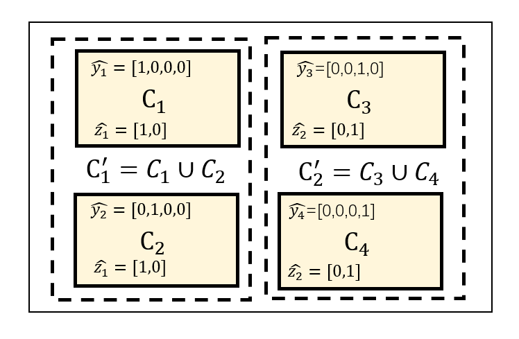
The classification probability for the merged class is a marginal probability
| (4) |
Also, the one-hot vector for a class is denoted as , which is -dimensional with and all others .
Consequently, we define marginal cross-entropy loss and marginal Dice loss as follows:
| (5) |
| (6) |
We use marginal cross entropy as an example to perform the gradient calculation. Firstly, referring to Eqs. (1) and (4), the gradient of the output of a softmax node to the network node is:
| (7) |
where is a boolean indicator function that tells if is in . and are the classification probabilities of regular and marginal softmax functions.The derivative gradient of to the network node is:
| (8) | ||||
where is the only class index that makes .
3.3 Exclusion loss
It happens in multi-organ segmentation tasks that some classes are mutually exclusive to each other. The exclusion loss is designed to add the exclusiveness as an additional prior knowledge on each image pixel. We define an exclusion subset for a class as , which comprises all (or a part of) the label indexes that are mutually exclusive with class . The exclusion label information is encoded as an N-dimensional vector , which is obtained as:
| (9) |
Note that is still an -dimensional vector, but it is not an one-hot vector any more. Fig.3 shows the procedure of applying exclusion loss. Assuming that organ classes , and are mutually exclusive, the labels of and form the exclusion subset .

We expect that the intersection between the segmentation prediction from the network and is as small as possible. Following the Dice coefficient, the formula for the exclusion Dice loss is given as:
| (10) |
The exclusion cross-entropy loss is defined accordingly:
| (11) |
where is introduced to avoid the trap of . We set .

| Network | Liver | Liver | Spleen | Spleen | Pancreas | Pancreas | L Kidney | R Kidney | L Kidney | R Kidney |
| : multiclass () | ||||||||||
| : binary liver () | ||||||||||
| : binary spleen () | ||||||||||
| : binary pancreas () | ||||||||||
| : binary kidney () | ||||||||||
| : binary liver () | ||||||||||
| : binary spleen () | ||||||||||
| : binary pancreas () | ||||||||||
| : ternary kidney () | ||||||||||
| : multiclass () | ||||||||||
| total # of training CT | 24 | 100 | 24 | 33 | 24 | 224 | 24 | 24 | 168 | 168 |
| total # of testing CT | 6 | 26 | 6 | 8 | 6 | 56 | 6 | 6 | 42 | 42 |
4 Experiments and Results
4.1 Problem setting and benchmark dataset
We consider a partially-supervised multi-organ segmentation task that is common in practice (such as Fig. 1). For each partially annotated image, we restrict it with only one label. For clarity of description, we assume that denotes the fully-labeled segmentation dataset and denotes a dataset of partially-annotated images that contain only a partial list of organ label(s). The datasets do not overlap in terms of their organ labels. For an image in , there is a ‘merged’ background, which is the union of real background and missing organ labels. We jointly learn a single segmentation network using , assisted by the proposed loss functions.
For our experiments, we choose liver, spleen, pancreas, left kidney and right kidney as the segmentation targets and use the following benchmark datasets.
-
1.
Dataset . We use Multi-Atlas Labeling Beyond the Cranial Vault - Workshop and Challenge [21] as fully annotated base dataset . It is composed of 30 CT images with segmentation labels of 13 organs, including liver, spleen, right kidney, left kidney, pancreas, and other organs (gallbladder, esophagus, stomach, aorta, inferior vena cava, portal vein and splenic vein, right adrenal gland, and left adrenal gland) we hereby ignore.
-
2.
Dataset . We refer to the task03 liver dataset from the Decathlon-10 [37] challenge as . It is composed of 130 CT’s with annotations for liver and liver cancer region. We merge the cancer label into the liver label and obtain a binary-class (liver vs background) dataset.
-
3.
Dataset . We refer to the task09 spleen dataset from the Decathlon-10 challenge as . It includes 41 CT’s with spleen segmentation label.
-
4.
Dataset . We refer to the task07 pancreas dataset from the Decathlon-10 challenge as . It includes 281 CT’s with pancreas and its cancer segmentation label. The cancer label is merged into the pancreas label to obtain a binary-class (pancreas vs background) dataset.
-
5.
Dataset . We refer to KiTS [18] challenge dataset as . Since the offered 210 CT segmentation makes no distinction between left and right kidneys, we manually divide it into left and right kidneys according to the connected component. Cancer label is merged into the according kidney label.
The spatial resolution of all these datasets are resampled to . We split the datesets into training and testing. we randomly choose 6 samples from , 26 samples from and 8 samples from , 56 samples from and 42 samples from as testing. The others are used for training. Table 2 also provides a summary description of the datasets.
| Dataset | Modiality | Num of labeled samples | Annotated organs | axis | image voxel range | spacing range |
|---|---|---|---|---|---|---|
| liver / right kidney / left kidney / | z | |||||
| MALBCVWC | CT | 30 | /pancreas /spleen / other structures | y | 512 | |
| x | 512 | |||||
| z | ||||||
| Decathlon-Liver | CT | 126 | liver | y | 512 | |
| x | 512 | |||||
| z | ||||||
| Decathlon-Spleen | CT | 41 | spleen | y | 512 | |
| x | 512 | |||||
| z | ||||||
| Decathlon-Pancreas | CT | 281 | pancreas | y | 512 | |
| x | 512 | |||||
| z | ||||||
| KiTS | CT | 210 | left kidney and right kidney | y | 512 | |
| x | 512 |
4.2 Segmentation networks
We set up the training of 10 deep segmentation networks for comparison as in Table 1.
-
1.
: a multiclass segmentation network based on .
-
2.
: a binary segmentation network for liver only based on .
-
3.
: a binary segmentation network for spleen only based on .
-
4.
: a binary segmentation network for pancreas only based on .
-
5.
: a ternary segmentation network for left kidney and right kidney only based on .
-
6.
: a binary segmentation network for liver only based on and . Note that the spleen, pancreas, left kidney and right kidney labels in are merged into background.
-
7.
: a binary segmentation network for spleen only based on and . Note that the liver, pancreas, left kidney and right kidney labels in are merged into background.
-
8.
: a binary segmentation network for pancreas only based on and . Note that the liver, spleen, left kidney and right kidney labels in are merged into background.
-
9.
: a ternary segmentation network for left kidney and right kidney only based on and . Note that the liver, spleen, pancreas labels in are merged into background.
-
10.
: a multi-class segmentation network based on , , , and .
4.3 Training procedure
For training the above networks except , we use the regular CE loss, regular Dice loss, and their combination. For training the network , when involves partial labels we need to invoke the marginal CE loss, marginal Dice loss, and their combination. Further, for we experiment the use of exclusion Dice loss and exclusion CE loss.
Considering the impact of the varying axial resolutions of different data sets in the original CT image on the training process, we resample the 3D CT image to and then extract the patch with the shape as input to illustrate the merit of our loss functions. For comparison, we use the same parameter settings in all networks; therefore there is no inference time difference among them. During training, we use 250 batches per epoch and 2 patches per batch. In order to ensure the stability of model training, we set the proportion of patches that contain foreground in each batch to be at least 33%. The initial learning rate of the network is 1e-1. Whenever the loss reduction is less than 1e-3 in consecutive 10 epochs, the learning rate decays by 20%.
We train 3D nnUNet [19] for all segmentation networks. We choose the 3D nnUNet because it is known to be a state-of-the-art segmentation network. While there are other network architectures [10] that might achieve comparable performance, we expect similar empirical observations from our ablation studies even based on the other networks.
For the network , we train it in two stages in order to prevent the instability caused by large loss value at the beginning of the training. In the first stage, we only use the fully annotated dataset . The goal is to minimize the regular loss function using the Adam optimizer. The purpose of the first phase is to give the network an initial weight on multi-class segmentation in order to prevent the large loss value when applying the marginal loss functions. In the second stage, each epoch is trained jointly using the union of five datasets. In each epoch, we randomly select 500 patches from each training dataset with a batch size of 2. Depending on the source of the slice, we use either the regular loss, if from , or the marginal loss and the exclusion loss, if from . In actual experiment, the first stage consists of 120 epochs and the second stage 80 epochs.
| : Multiclass () | |||||||||||
| Loss | Liver | Liver | Spleen | Spleen | Pancreas | Pancreas | L Kidney | R Kidney | L Kidney | R Kidney | All |
| rCE | .846 | ||||||||||
| rDC | .826 | ||||||||||
| rCE+rDC | .874 | ||||||||||
| Loss | Liver | Liver | Spleen | Spleen | Pancreas | Pancreas | L Kidney | R Kidney | L Kidney | R Kidney | All |
| rCE | .835 | ||||||||||
| rDC | .839 | ||||||||||
| rCE+rDC | .851 | ||||||||||
| Loss | Liver | Liver | Spleen | Spleen | Pancreas | Pancreas | L Kidney | R Kidney | L Kidney | R Kidney | All |
| rCE | .877 | ||||||||||
| rDC | .879 | ||||||||||
| rCE+rDC | .900 | ||||||||||
| : Multiclass () | |||||||||||
| Loss | Liver | Liver | Spleen | Spleen | Pancreas | Pancreas | L Kidney | R Kidney | L Kidney | R Kidney | All |
| mCE | .873 | ||||||||||
| mDC | .876 | ||||||||||
| mCE+mDC | .921 | ||||||||||
| mCE+mDC+eCE+eDC | .931 | ||||||||||
| : Multiclass () | |||||||||||
| Loss | Liver | Liver | Spleen | Spleen | Pancreas | Pancreas | L Kidney | R Kidney | L Kidney | R Kidney | All |
| rCE | 10.82 | ||||||||||
| rDC | 10.34 | ||||||||||
| rCE+rDC | 9.33 | ||||||||||
| Loss | Liver | Liver | Spleen | Spleen | Pancreas | Pancreas | L Kidney | R Kidney | L Kidney | R Kidney | All |
| rCE | 12.49 | ||||||||||
| rDC | 12.38 | ||||||||||
| rCE+rDC | 10.73 | ||||||||||
| Loss | Liver | Liver | Spleen | Spleen | Pancreas | Pancreas | L Kidney | R Kidney | L Kidney | R Kidney | All |
| rCE | 9.86 | ||||||||||
| rDC | 9.59 | ||||||||||
| rCE+rDC | 6.64 | ||||||||||
| : Multiclass () | |||||||||||
| Loss | Liver | Liver | Spleen | Spleen | Pancreas | Pancreas | L Kidney | R Kidney | L Kidney | R Kidney | All |
| mCE | 9.81 | ||||||||||
| mDC | 9.48 | ||||||||||
| mCE+mDC | 4.43 | ||||||||||
| mCE+mDC+eCE+eDC | 4.02 | ||||||||||
4.4 Ablation studies
We use two standard metrics for gauging the performance of a segmentation method: Dice coefficient and Hausdorff distance (HD). A higher Dice coefficient or a lower HD means a better segmentation result. Table 3 shows the mean and standard deviation of Dice coefficients of the results obtained by the deep segmentation networks under different loss combinations and with different dataset usages, from which we make the following observations.
The effect of pooling together more data. The experimental results obtained by the models jointly trained from combinations of the datasets and are generally better than those by the models trained from a single labeled dataset alone. As shown in Table 3 and Table 4, when comparing the performance of vs , the former generally outperforms the latter. For example, when using rCE+rDC as the loss, the mean Dice coefficient is boosted from .851 to .900 (the according HD is reduced by 37.5%). When comparing the performance of vs , again the former is better than the latter, the mean dice coefficient is increased from .874 to .900 (the according HD is reduced by 28.7%).
The importance of CE and Dice losses. When comparing the importance of CE and Dice losses, in general, it is inconclusive which one is better, depending on the setup. For example, the Dice loss works better on liver segmentation while the CE loss significantly outperforms the Dice loss on left kidney segmentation. Also fusing CE and Dice losses is in general beneficial in terms of our results as it usually brings a gain in segmentation performance. For example, when using , the average dice loss reaches .874 for rCE+rDC, while that for rCE and rDC is .846 and .826, respectively.
| mLoss:eLoss | Liver | Liver | Spleen | Spleen | Pancreas | Pancreas | L Kidney | R Kidney | L Kidney | R Kidney | All |
|---|---|---|---|---|---|---|---|---|---|---|---|
| 4:1 | .910 | ||||||||||
| 3:1 | .916 | ||||||||||
| 2:1 | .926 | ||||||||||
| 1:1 | |||||||||||
| 1:2 | .931 | ||||||||||
| 1:3 | .920 | ||||||||||
| 1:4 | .913 | ||||||||||
| 1:0 | .921 | ||||||||||
| 0:1 | .897 | ||||||||||
| 4:1 | 6.17 | ||||||||||
| 3:1 | 5.00 | ||||||||||
| 2:1 | 4.43 | ||||||||||
| 1:1 | 5.46 | ||||||||||
| 1:2 | 4.02 | ||||||||||
| 1:3 | 5.25 | ||||||||||
| 1:4 | 6.86 | ||||||||||
| 1:0 | 4.43 | ||||||||||
| 0:1 | 6.98 |
| full : partial | Total # of annotated organs | Liver | Spleen | Pancreas | L Kidney | R Kidney | All |
|---|---|---|---|---|---|---|---|
| 24/00 | 120 | .874 | |||||
| 19/05 | 100 | .859 | |||||
| 14/10 | 80 | .818 | |||||
| 09/15 | 60 | .798 | |||||
| 04/20 | 40 | .774 | |||||
| 24/00 | 120 | 9.33 | |||||
| 19/05 | 100 | 12.00 | |||||
| 14/10 | 80 | 15.71 | |||||
| 09/15 | 60 | 14.37 | |||||
| 04/20 | 40 |
The combined effect of data pooling and using marginal loss. It is evident that the segmentation network exhibits a significant performance gain, enabled by joint training on the five datasets. It brings a 4.7% increases (.921 vs .874) in average dice coefficient for test images when compared with , which is trained on alone when using the dice loss and CE. Specifically, it brings an average 5.45% improvement on liver segmentation (.965 vs .960 on test images and .954 vs .850 on test images), an average 4.0% improvement on spleen segmentation (.891 vs .859 on test images and .966 vs .918 on test images), an average 5.05% improvement on pancreas segmentation (.807 vs .802 on test images and .791 vs .695 on test images), and an average 4.45% improvement on kidney segmentation (.945 vs .934 on test images and .974 vs .896 on test images).
The effect of exclusion loss. In addition, the exclusion loss brings significant performance boosting. The final results have been effectively improved by an average of 1.0% increases of Dice coefficient compared to the results obtained without the exclusion loss. This confirms that our proposed exclusion loss can promote the proper learning of the mutual exclusion between two labels. But it should be noted that exclusion loss is more like an auxiliary loss for partial label learning.
In sum, with the help of our newly proposed marginal loss and exclusion loss which enable the joint training of both fully labelled and partially labelled dataset, it brings a 3.1% increase (.931 vs .900) in dice coefficient. Such a performance improvement is essentially a free boost because these datasets are existent and already labeled.
Hausdorff distance. Table 4 shows the mean Hausdorff distance of the testing results, from which similar observations are made. Notably, jointly training from the five datasets, enabled by the marginal loss, can effectively increase the performances, especially it reduces the average distance from 9.33 to 4.43 (a 52.5% reduction) when using the Dice loss. Adding exclusion dice can further improve the performances (4.43 to 4.02, another 9.3% reduction). The main reason for the big HD values for say spleen is that sometime a small part of predicted spleen segmentation appears in non-spleen region. This does not affect the Dice coefficient but creates an outlier HD value.
The impact of loss weight. In order to further explore the impact of marginal loss and exclusion loss on the performance, we set up the training of a series of models to understand the influence of the weight ratio of marginal and exclusion losses. All the models are trained on the union of and all the partially-annotated datasets. We experiment with ten different weight ratios: 4:1, 3:1, 2:1, 1:1, 1:2, 1:3, 1:4, 1:0, and 0:1. The dice coefficients and Hausdorff distances are reported in Table 5. Results demonstrate that a weight ratio of 1:2 achieves the best results on almost all the metrics. It is interesting to observe that, when only using exclusion loss (experiment with a weight of 0:1), there is nearly no performance improvement on pancreas and kidney comparing with , which uses only for training (as in Tables 3 and 4). This indicates that exclusion loss is more suitable as an auxiliary loss to be used with marginal loss together.
The effect of the number of annotations. Finally, we perform a group of tests to measure the sensitivity of performance with the number of data annotation increases. We randomly split the fully annotated dataset into a training set with 24 samples and a testing set with six samples and leave the testing set untouched. In the five sets of experiments reported in Table 6 , we alter the training set by replacing some fully labeled data with single labeled data, while keeping the total number of the training data unchanged. For example, for a ‘14/10’ split, we have 14 fully labels images with 5 organs, and the rest of 10 images are further randomly divided into 5 single-label groups of 2 images. For the 1st group, we can use its liver annotation. Similarly we use only the spleen, pancreas, left kidney, and right kidney labels for the 2nd to the 5th groups, respectively. As a result, we have a total of 14*5+2*5=80 annotated organs. Results in Table 6 confirm that the dice coefficient consistently decreases as the amount of annotation decreases, which is as expected.
4.5 Comparison with state-of-the-art
Our model is also compared with the other partially-supervised segmentation networks. The results are shown in Table 7. The Prior-aware Neural Network (PaNN) refers to the work by Zhou et al. [52] which adds a prior-aware loss to learn partially labeled data. The pyramid input and pyramid output (PIPO) refers to the work by Fang et al. [10] which develops a multi-scale structure as well as target adaptive loss to enable learning partially labeled data. Our work achieves a significantly better performance than these two methods. The average Dice reaches 0.931 for our model, while that for PaNN and PIPO is 0.906 and 0.907, respectively. Our method also greatly reduce the mean Hausdorff distance by 24.0% comparing with PaNN and 40.0% comparing with PIPO. Specifically, our method achieves slight better (except for Liver) performance for large organs such as liver and spleen, but it brings a significant performance boost on small organs such as pancreas, left and right kidneys. Our work performs consistently better than the PIPO method on all the organs regardless the datasets, the improvement may be due to the use of 3D model as well as the exclusion loss.
Fig. 4 presents visualization of sample results of different methods. With the assistance of auxiliary datasets, the performances are significantly improved. Especially, there are situations occurring on all the other methods that the predicted organ region enters a different organ, which results a large HD value. The exclusion loss used in our method can effectively reduce such an error and greatly improve the HD performance. Besides, our method can achieve more meticulous segmentation results on some small organs such as pancreas and kidney, especially when there are small holes around the organ center.


5 Discussions and Conclusions
In this paper, we propose two new types of loss function that can be used for learning a multi-class segmentation network based on multiple datasets with partial organ labels. The marginal loss enables the learning due to the presence of ‘merged’ labels, while the exclusion loss promotes the learning by adding the mutual exclusiveness as prior knowledge on each labeled image pixel. Our extensive experiments on five benchmark datasets clearly confirm that a significant performance boost is achieved by using marginal loss and exclusion loss. Our method also greatly outperforms existing frameworks for partially annotated data learning.
However, our proposed method is far from perfect. Fig. 5 shows two typical failure cases. In the left image, the background has similar features to liver so the liver prediction on the right side is wrong. In the right image, our method still has some misjudgment on spleen and pancreas. We will generalize the current method for improved segmentation performances by incorporating more knowledge about the organs, such as using shape adversarial prior [49]. Furthermore, in future we will extend the marginal loss and exclusion loss on other tasks for partially labeled annotated learning and explore the use of other loss functions.
References
- Berman et al. [2018] Berman, M., Rannen Triki, A., Blaschko, M.B., 2018. The lovász-softmax loss: A tractable surrogate for the optimization of the intersection-over-union measure in neural networks, in: Proceedings of the IEEE Conference on Computer Vision and Pattern Recognition, pp. 4413–4421.
- Binder et al. [2019] Binder, T., Tantaoui, E.M., Pati, P., Catena, R., Set-Aghayan, A., Gabrani, M., 2019. okada2015abdominal. Frontiers in Medicine 6, 173.
- Cerrolaza et al. [2015] Cerrolaza, J.J., Reyes, M., Summers, R.M., González-Ballester, M.Á., Linguraru, M.G., 2015. Automatic multi-resolution shape modeling of multi-organ structures. Medical image analysis 25, 11–21.
- Chen et al. [2018] Chen, H., Dou, Q., Yu, L., Qin, J., Heng, P.A., 2018. Voxresnet: Deep voxelwise residual networks for brain segmentation from 3d mr images. NeuroImage 170, 446–455.
- Chen et al. [2012] Chen, X., Udupa, J.K., Bagci, U., Zhuge, Y., Yao, J., 2012. Medical image segmentation by combining graph cuts and oriented active appearance models. IEEE transactions on image processing 21, 2035–2046.
- Chu et al. [2013] Chu, C., Oda, M., Kitasaka, T., Misawa, K., Fujiwara, M., Hayashi, Y., Nimura, Y., Rueckert, D., Mori, K., 2013. Multi-organ segmentation based on spatially-divided probabilistic atlas from 3d abdominal ct images, in: International conference on medical image computing and computer-assisted intervention, Springer. pp. 165–172.
- Cootes et al. [2001] Cootes, T.F., Edwards, G.J., Taylor, C.J., 2001. Active appearance models. IEEE Transactions on pattern analysis and machine intelligence 23, 681–685.
- Cour et al. [2011] Cour, T., Sapp, B., Taskar, B., 2011. Learning from partial labels. Journal of Machine Learning Research 12, 1501–1536. URL: http://jmlr.org/papers/v12/cour11a.html.
- Dmitriev and Kaufman [2019] Dmitriev, K., Kaufman, A.E., 2019. Learning multi-class segmentations from single-class datasets, in: The IEEE Conference on Computer Vision and Pattern Recognition (CVPR).
- Fang and Yan [2020] Fang, X., Yan, P., 2020. Multi-organ segmentation over partially labeled datasets with multi-scale feature abstraction. IEEE Transactions on Medical Imaging , 1–1doi:10.1109/TMI.2020.3001036.
- Gibson et al. [2018] Gibson, E., Giganti, F., Hu, Y., Bonmati, E., Bandula, S., Gurusamy, K., Davidson, B., Pereira, S.P., Clarkson, M.J., Barratt, D.C., 2018. Automatic multi-organ segmentation on abdominal ct with dense v-networks. IEEE transactions on medical imaging 37, 1822–1834.
- Ginneken et al. [2011] Ginneken, B.V., Schaefer-Prokop, C.M., Prokop, M., 2011. Computer-aided diagnosis: How to move from the laboratory to the clinic. Radiology 261, 719–732.
- Hadsell et al. [2006] Hadsell, R., Chopra, S., LeCun, Y., 2006. Dimensionality reduction by learning an invariant mapping, in: 2006 IEEE Computer Society Conference on Computer Vision and Pattern Recognition (CVPR’06), IEEE. pp. 1735–1742.
- He et al. [2015] He, B., Huang, C., Jia, F., 2015. Fully automatic multi-organ segmentation based on multi-boost learning and statistical shape model search. CEUR Workshop Proceedings 1390, 18–21.
- He et al. [2019] He, Z.F., Yang, M., Gao, Y., Liu, H.D., Yin, Y., 2019. Joint multi-label classification and label correlations with missing labels and feature selection. Knowledge-Based Systems 163, 145–158.
- Heimann and et al. [2009] Heimann, T., et al., 2009. Comparison and Evaluation of Methods for Liver Segmentation From CT Datasets. IEEE Transactions on Medical Imaging 28, 1251–1265.
- Heimann and Meinzer [2009] Heimann, T., Meinzer, H.P., 2009. Statistical shape models for 3d medical image segmentation: a review. Medical image analysis 13, 543–563.
- Heller et al. [2019] Heller, N., Sathianathen, N., Kalapara, A., Walczak, E., Moore, K., Kaluzniak, H., Rosenberg, J., Blake, P., Rengel, Z., Oestreich, M., et al., 2019. The kits19 challenge data: 300 kidney tumor cases with clinical context, ct semantic segmentations, and surgical outcomes. arXiv preprint arXiv:1904.00445 .
- Isensee et al. [2018] Isensee, F., Petersen, J., Klein, A., Zimmerer, D., Jaeger, P.F., Kohl, S., Wasserthal, J., Koehler, G., Norajitra, T., Wirkert, S., et al., 2018. nnu-net: Self-adapting framework for u-net-based medical image segmentation. arXiv preprint arXiv:1809.10486 .
- Kohlberger et al. [2011] Kohlberger, T., Sofka, M., Zhang, J., Birkbeck, N., Wetzl, J., Kaftan, J., Declerck, J., Zhou, S.K., 2011. Automatic multi-organ segmentation using learning-based segmentation and level set optimization, in: Fichtinger, G., Martel, A., Peters, T. (Eds.), Medical Image Computing and Computer-Assisted Intervention, Springer Berlin Heidelberg, Berlin, Heidelberg. pp. 338–345.
- Landman et al. [2017] Landman, B., Xu, Z., Igelsias, J., Styner, M., Langerak, T., Klein, A., 2017. Multi-atlas labeling beyond the cranial vault-workshop and challenge.
- Lay et al. [2013] Lay, N., Birkbeck, N., Zhang, J., Zhou, S.K., 2013. Rapid multi-organ segmentation using context integration and discriminative models, in: Gee, J.C., Joshi, S., Pohl, K.M., Wells, W.M., Zöllei, L. (Eds.), Information Processing in Medical Imaging, Springer Berlin Heidelberg, Berlin, Heidelberg. pp. 450–462.
- Li et al. [2018] Li, Y., Gao, F., Ou, Z., Sun, J., 2018. Angular softmax loss for end-to-end speaker verification, in: 2018 11th International Symposium on Chinese Spoken Language Processing (ISCSLP), IEEE. pp. 190–194.
- Lin et al. [2017] Lin, T.Y., Goyal, P., Girshick, R., He, K., Dollár, P., 2017. Focal loss for dense object detection, in: Proceedings of the IEEE international conference on computer vision, pp. 2980–2988.
- Liu et al. [2016] Liu, W., Wen, Y., Yu, Z., Yang, M., 2016. Large-margin softmax loss for convolutional neural networks, in: International Conference on Machine Learning, p. 7.
- Liu et al. [2020] Liu, Y., Gargesha, M., Qutaish, M., Zhou, Z., Scott, B., Yousefi, H., Lu, Z., Wilson, D.L., 2020. Deep learning based multi-organ segmentation and metastases segmentation in whole mouse body and the cryo-imaging cancer imaging and therapy analysis platform (citap), in: Medical Imaging 2020: Biomedical Applications in Molecular, Structural, and Functional Imaging, International Society for Optics and Photonics. p. 113170V.
- Lombaert et al. [2014] Lombaert, H., Zikic, D., Criminisi, A., Ayache, N., 2014. Laplacian forests: Semantic image segmentation by guided bagging, in: International Conference on Medical Image Computing and Computer-assisted Intervention.
- Long et al. [2015] Long, J., Shelhamer, E., Darrell, T., 2015. Fully convolutional networks for semantic segmentation, in: The IEEE Conference on Computer Vision and Pattern Recognition (CVPR).
- Lu et al. [2012] Lu, C., Zheng, Y., Birkbeck, N., Zhang, J., Kohlberger, T., Tietjen, C., Boettger, T., Duncan, J.S., Zhou, S.K., 2012. Precise segmentation of multiple organs in ct volumes using learning-based approach and information theory, in: International Conference on Medical Image Computing and Computer-Assisted Intervention, Springer. pp. 462–469.
- Okada et al. [2015] Okada, T., Linguraru, M.G., Hori, M., Summers, R.M., Tomiyama, N., Sato, Y., 2015. Abdominal multi-organ segmentation from ct images using conditional shape–location and unsupervised intensity priors. Medical image analysis 26, 1–18.
- Okada et al. [2012] Okada, T., Linguraru, M.G., Hori, M., Suzuki, Y., Summers, R.M., Tomiyama, N., Sato, Y., 2012. Multi-organ segmentation in abdominal ct images, in: 2012 Annual International Conference of the IEEE Engineering in Medicine and Biology Society, IEEE. pp. 3986–3989.
- Ronneberger et al. [2015] Ronneberger, O., Fischer, P., Brox, T., 2015. U-net: Convolutional networks for biomedical image segmentation, in: International Conference on Medical image computing and computer-assisted intervention, Springer. pp. 234–241.
- Salehi et al. [2017] Salehi, S.S.M., Erdogmus, D., Gholipour, A., 2017. Tversky loss function for image segmentation using 3d fully convolutional deep networks, in: International Workshop on Machine Learning in Medical Imaging, Springer. pp. 379–387.
- Saxena et al. [2016] Saxena, S., Sharma, N., Sharma, S., Singh, S., Verma, A., 2016. An automated system for atlas based multiple organ segmentation of abdominal ct images. British Journal of Mathematics and Computer Science 12, 1–14. doi:10.9734/BJMCS/2016/20812.
- Schroff et al. [2015] Schroff, F., Kalenichenko, D., Philbin, J., 2015. Facenet: A unified embedding for face recognition and clustering, in: Proceedings of the IEEE conference on computer vision and pattern recognition, pp. 815–823.
- Shimizu et al. [2007] Shimizu, A., Ohno, R., Ikegami, T., Kobatake, H., Nawano, S., Smutek, D., 2007. Segmentation of multiple organs in non-contrast 3d abdominal ct images. International journal of computer assisted radiology and surgery 2, 135–142.
- Simpson et al. [2019] Simpson, A.L., Antonelli, M., Bakas, S., Bilello, M., Farahani, K., Van Ginneken, B., Kopp-Schneider, A., Landman, B.A., Litjens, G., Menze, B., et al., 2019. A large annotated medical image dataset for the development and evaluation of segmentation algorithms. arXiv preprint arXiv:1902.09063 .
- Suzuki et al. [2012] Suzuki, M., Linguraru, M.G., Okada, K., 2012. Multi-organ segmentation with missing organs in abdominal ct images, in: International Conference on Medical Image Computing and Computer-Assisted Intervention, Springer. pp. 418–425.
- Sykes [2014] Sykes, J., 2014. Reflections on the current status of commercial automated segmentation systems in clinical practice. Journal of Medical Radiation Sciences 61, 131–134.
- Taghanaki et al. [2019] Taghanaki, S.A., Zheng, Y., Zhou, S.K., Georgescu, B., Sharma, P., Xu, D., Comaniciu, D., Hamarneh, G., 2019. Combo loss: Handling input and output imbalance in multi-organ segmentation. Computerized Medical Imaging and Graphics 75, 24–33.
- Tong et al. [2015] Tong, T., Wolz, R., Wang, Z., Gao, Q., Misawa, K., Fujiwara, M., Mori, K., Hajnal, J.V., Rueckert, D., 2015. Discriminative dictionary learning for abdominal multi-organ segmentation. Medical image analysis 23, 92–104.
- Wang et al. [2018] Wang, H., Wang, Y., Zhou, Z., Ji, X., Gong, D., Zhou, J., Li, Z., Liu, W., 2018. Cosface: Large margin cosine loss for deep face recognition, in: Proceedings of the IEEE Conference on Computer Vision and Pattern Recognition, pp. 5265–5274.
- Wang et al. [2019] Wang, Y., Zhou, Y., Shen, W., Park, S., Fishman, E.K., Yuille, A.L., 2019. Abdominal multi-organ segmentation with organ-attention networks and statistical fusion. Medical image analysis 55, 88–102.
- Wen et al. [2016] Wen, Y., Zhang, K., Li, Z., Qiao, Y., 2016. A discriminative feature learning approach for deep face recognition, in: European conference on computer vision, Springer. pp. 499–515.
- Wolz et al. [2013] Wolz, R., Chu, C., Misawa, K., Fujiwara, M., Mori, K., Rueckert, D., 2013. Automated abdominal multi-organ segmentation with subject-specific atlas generation. IEEE transactions on medical imaging 32, 1723–1730.
- Wu et al. [2015] Wu, B., Lyu, S., Hu, B.G., Ji, Q., 2015. Multi-label learning with missing labels for image annotation and facial action unit recognition. Pattern Recognition 48, 2279–2289.
- Xiao et al. [2019] Xiao, L., Zhu, C., Liu, J., Luo, C., Liu, P., Zhao, Y., 2019. Learning from suspected target: Bootstrapping performance for breast cancer detection in mammography, in: Medical Image Computing and Computer Assisted Intervention, Springer International Publishing, Cham. pp. 468–476.
- Xu et al. [2015] Xu, Z., Burke, R.P., Lee, C.P., Baucom, R.B., Poulose, B.K., Abramson, R.G., Landman, B.A., 2015. Efficient multi-atlas abdominal segmentation on clinically acquired ct with simple context learning. Medical image analysis 24, 18–27.
- Yang et al. [2017] Yang, D., Xu, D., Zhou, S.K., Georgescu, B., Chen, M., Grbic, S., Metaxas, D., Comaniciu, D., 2017. Automatic liver segmentation using an adversarial image-to-image network, in: Descoteaux, M., Maier-Hein, L., Franz, A., Jannin, P., Collins, D.L., Duchesne, S. (Eds.), Medical Image Computing and Computer Assisted Intervention, Springer International Publishing, Cham. pp. 507–515.
- Yu et al. [2014] Yu, H.F., Jain, P., Kar, P., Dhillon, I., 2014. Large-scale multi-label learning with missing labels, in: International conference on machine learning, pp. 593–601.
- Zhao et al. [2019] Zhao, A., Balakrishnan, G., Durand, F., Guttag, J.V., Dalca, A.V., 2019. Data augmentation using learned transformations for one-shot medical image segmentation, in: Proceedings of the IEEE conference on computer vision and pattern recognition, pp. 8543–8553.
- Zhou et al. [2019] Zhou, Y., Li, Z., Bai, S., Wang, C., Chen, X., Han, M., Fishman, E., Yuille, A.L., 2019. Prior-aware neural network for partially-supervised multi-organ segmentation, in: Proceedings of the IEEE International Conference on Computer Vision, pp. 10672–10681.
- Zhu et al. [2018] Zhu, P., Xu, Q., Hu, Q., Zhang, C., Zhao, H., 2018. Multi-label feature selection with missing labels. Pattern Recognition 74, 488–502.