Mapping Incidence and Prevalence Peak Data for SIR Forecasting Applications
Abstract
Infectious disease modeling and forecasting have played a key role in helping assess and respond to epidemics and pandemics. Recent work has leveraged data on disease peak infection and peak hospital incidence to fit compartmental models for the purpose of forecasting and describing the dynamics of a disease outbreak. Incorporating these data can greatly stabilize a compartmental model fit on early observations, where slight perturbations in the data may lead to model fits that project wildly unrealistic peak infection. We introduce a new method for incorporating historic data on the value and time of peak incidence of hospitalization into the fit for a Susceptible-Infectious-Recovered (SIR) model by formulating the relationship between an SIR model’s starting parameters and peak incidence as a system of two equations that can be solved computationally. This approach is assessed for practicality in terms of accuracy and speed of computation via simulation. To exhibit the modeling potential, we update the Dirichlet-Beta State Space modeling framework to use hospital incidence data, as this framework was previously formulated to incorporate only data on total infections.
keywords:
, , , , , , and
1 Introduction
Compartmental models have seen broad usage at the onset of several disease outbreaks in the last century as a means to project expected numbers of infected and to drive healthcare response. Broadly speaking, a compartmental model describes the dynamics of a disease spread by breaking a population into set categories and modeling the process by which individuals transition through these categories. Perhaps the most basic is the Kermack–McKendrick model, often called the SIR or Susceptible-Infectious-Recovered model, which models the movement of subjects from being Susceptible, to Infected (and contagious), and then to Removed (Kermack, McKendrick and Walker, 1927). Since the development of the SIR model, further research has extended the idea to include additional compartments, such as the Exposed category in the SEIR model – where a subject has been exposed to the disease but is not yet infectious – and the ability to move back to the Susceptible category in the SEIS model (see Walter and Contreras (1999); Hethcote (2000) for an overview of each). Compartmental models have been applied to projection tasks such as the 2014-15 Ebola epidemic (Chretien, Riley and George, 2015), the 2009 A/H1N1 influenza pandemic (Nsoesie et al., 2014), several HIV outbreaks (Anderson, 1988; Golub, Gorr and Gould, 1993; Nyabadza, Mukandavire and Hove-Musekwa, 2011), the recent COVID-19 pandemic (Zhao and Chen, 2020; Cooper, Mondal and Antonopoulos, 2020; Zhang et al., 2022), and many other epidemiological projection tasks in the last century (see, for instance, Guanghong et al. (2004); LaDeau et al. (2011); Zhan et al. (2019) and references therein).
The elegance of compartmental models is in their succinct ability to describe the state of a population in terms of how subjects transfer to and from the different categories, and thus fitting these models requires estimation of interpretable quantities such as rates of infection and recovery. For instance, denote the proportion of the population in the susceptible, infectious, and removed compartments by and respectively, such that for all . Then the SIR model is determined by the equations
| (1a) | ||||
| (1b) | ||||
| (1c) | ||||
where is the disease transmission rate and is the rate of recovery. If one knew these two rates, and the initial number of individuals in each category – and – the numbers could be numerically simulated for any time-point . While modern computational tools do make simulating these quantities feasible, the need to simulate the entire system numerically to get the exact counts in each compartment is challenging. That is, fitting these models to data and can be computationally expensive for more intricate compartmental structures. Researchers have determined analytic solutions for the entire SIR model (explicit forms/approximations to the number of susceptible, infected, and removed at a specific time) that do not require numeric simulation (Harko, Lobo and Mak, 2014; Schlickeiser and Kröger, 2021; Carvalho and Gonçalves, 2021). However, these solutions involve reparameterizing the time axis, and explicit calculations back onto the original time axis require numeric integration or approximation methods. Similar approaches are also used to obtain exact and approximate solutions to the more complicated compartmental models, such as the SEIR model (Wang, Wei and Zhang, 2014; Piovella, 2020) and the SIRS model (Acedo, González-Parra and Arenas, 2010).
Analytic maps from the initial starting parameters of an SIR curve to quantities of interest (QoIs) – such as the value of the peak of the infected curve and the limiting number of susceptible individuals – were developed as early as the mid-1900s (Kendall, 1956; Bailey, 1957; Hethcote, 1976). The focus on these quantities has generally been motivated by their usefulness to making public health decisions. For instance, in papers such as Hethcote (2000) and Weiss (2013), the maximum value of the infected compartment (not the time of maximum infection) was studied for the purpose of informing public health officials of the maximum number of infections after the initial estimation of the disease transmission and recovery rates, since knowing this maximum quantity informs how many hospital beds might be needed. The authors in Castro et al. (2020) point out that the time of peak infection is also informative for healthcare officials, and they develop an analytic form for the peak time of infection using an approximation of the SIR curve. An exact form for the peak infection time is available in Kendall (1956) and Deakin (1975), albeit in terms of an integral without a closed form. Several modern papers study fast approximations to the integral form for peak infection time (Cadoni and Gaeta, 2020; Turkyilmazoglu, 2021), using the previously-mentioned analytic solutions to the SIR model. These different approximations for peak infection time are evaluated and compared in Kröger, Turkyilmazoglu and Schlickeiser (2021).
Some recent papers study SIR curve QoIs for inferential tasks related to modeling an epidemic (Miller, 2009; Lang et al., 2018). In Amaro (2023), the Gumbel distribution is suggested as a good approximation of the infection curve in an SIR model, and maps between the SIR curve parameters and peak value/time are used to develop Method of Moments estimators of the Gumbel parameters. The Gumbel distribution is then used to approximate the exact solution of the SIR model. In Osthus et al. (2017), the relationship between peak infection value and the SIR parameters is used to incorporate historical data on epidemic peaks into the inferential task of fitting an SIR curve during the early stages of an epidemic. The authors point out that an SIR curve is sensitive to small perturbations in the transmission and recovery rates, and that incorporating these data discourages models that well-represent early data but drastically over-predict the peak infection value. In McAndrew et al. (2024), both historic and surveyed QoIs are used to constrain an SEIRH model (where the added “H” category refers to people hospitalized at a given time) in much the same way as Osthus et al. (2017).

Both Amaro (2023) and Osthus et al. (2017) use information on peak infection value and time to inform the modeling of a pandemic and epidemic, respectively. Since most modern monitoring systems approximate the daily number of new cases of a disease, called incidence, this is not the most practically useful development. The number of infected individuals at any given time, called prevalence, is typically an unobserved quantity (Noordzij et al., 2010). For examples of all quantities in an SIR curve on a fixed time axis, see Figure 1. Note that peak prevalence and peak incidence need not occur at the same time, and that it is mathematically possible for the incidence to be greater than prevalence (as visualized on the right side of Figure 1). This being said, in most disease outbreaks of note, prevalence is typically greater than incidence.
The model in McAndrew et al. (2024) incorporates incidence QoI data by extending the parameter space to include peak incidence value (PIV) and peak incidence time (PIT) and by defining a prior on these values using either historic or survey data. While this model achieves a similar goal to the ultimate goal of this paper, its main distinction is that that it requires an importance sampling scheme to fit, which we outline here for completeness: priors on the rate parameters and initial values for the compartmental model are used to sample proposal values, the entire system is numerically simulated to determine the (PIV, PIT), then the likelihood of this system is determined via the prior probability of (PIV, PIT). Note that while this need not be true for the SEIRH model considered in McAndrew et al. (2024) (since it is not an SIR model), defining both a prior on the rate parameters and on PIV and PIT for an SIR model is redundant given the initial values , , and , since a given set of starting parameters should immediately determine these QoIs.
Incorporating historical peak values and times of an outbreak into a Bayesian compartmental forecasting model via prior specifications is highly useful to constrain forecasts111For a review of the differences between disease forecasts and disease projections, see Massad et al. (2005)., especially early in the outbreak (see Osthus et al. (2017), Osthus et al. (2019), and McAndrew et al. (2024)). Relating these historical QoIs requires determining a relationship between historical peak values and times as well as the parameters and initial conditions of the compartmental model (e.g., the SIR model). The challenge lies in this relationship. Analytically, this relationship is known for observed peak prevalence value (PPV) and peak prevalence time (PPT). However, almost all infectious disease data is of incidence. Despite being principally unsound, the data application in Osthus et al. (2017) treated incidence data as if it were prevalence in order to use the known analytic relationships. In this paper, we make three contributions. First, we develop the methods to map peak values and times of incidence to the parameters of the SIR model, given the initial conditions. Second, we demonstrate how to incorporate these new mappings into the model of Osthus et al. (2017) and provide the code used to do so. Third, we compare the forecasts of the modeling framework of Osthus et al. (2017) using both incidence data as incidence, and using the misspecified prevalence data. In addition to comparing these forecasts, we show that if SIR parameter inference is desired, then mistaking incidence data for prevalence data will result in biased estimation.
This paper is outlined as follows. In Section 2, we review existing methods for mapping SIR parameters to peak/time of prevalence. In Section 3, we develop identical maps for incidence, then provide methods for inverting these maps for both incidence and prevalence. In Section 4, we develop and improve upon the modeling framework in Osthus et al. (2017) to incorporate historic incidence peak/time data when fitting an SIR curve. We apply this model to influenza data in Section 5.
2 Analytic Solutions to the SIR Equations for Incorporating Prevalence Data
The system (1a)-(1c) can be solved analytically for all time by reparameterizing the time axis to be instead in terms of the number of individuals removed from the system beyond the initial amount in the Removed category ,
| (2a) | ||||
| (2b) | ||||
| (2c) | ||||
where is the inverse of the map
| (3) |
where The above form for the SIR dynamics is particularly useful since it allows one to calculate the number of individuals in each category without numerically simulating the entire system. The major drawback of this form is that mapping values back to an interpretable time requires one to approximate the integral in (3), since this integral is nonelementary. There exist other methods that derive an analytic solution to the SIR system (Harko, Lobo and Mak, 2014). We use this formulation since it is well-known (having been originally developed in Kendall (1956)), and because it simplifies the calculation of SIR curve QoIs, such as PPV and PPT. For instance, the maximum of (2b) with respect to occurs at
| (4) |
which can be derived via straightforward calculus. PPT can then be approximated from (3), and PPV calculated from (2b).
The process above of calculating PPV and PPT, denoted from the initial starting parameters can be reversed for fixed . That is, given , we propose a method to calculate . Define as
| (5) |
The quantity is more widely known as the basic reproduction number, which measures the average number of additional infections generated by a single new infection (Cadoni and Gaeta, 2020). Plugging (4) into (2b) gives
| (6) |
From here, setting and solving for is a (piecewise) convex optimization problem, which is typically fast and accurate computationally. Note that a change of variables for (3) gives
| (7) |
and that . Thus, once the value of is approximated, (7) can be evaluated to get . Since is assumed known a priori, the values of and can be obtained via arithmetic.
We introduce the above derivations not only because they will be used in the next Section, but also to motivate the type of calculation we aim to develop in this paper. While the above approach still requires computational methods to map from PPV and PPT to the SIR model parameters, this approach is much more direct than the brute force method of simulating several combinations until a prevalence curve with a peak sufficiently near is discovered (Prangle, 2016).
3 Mapping Incidence Data to SIR Parameters
As mentioned above, a primary focus of this work will be to develop maps between PIV and PIT and the initial SIR curve parameters. In this direction, one can derive an equivalent formulation of the SIR dynamics in (1a) - (1c) by replacing (1b) with
| (8) |
Putting (8) into words, prevalence is equal to the prevalence at the last time step, plus those in the infected category that infect those in the susceptible category, minus the number in the infected category that are removed from the system. The form for prevalence in (8) is particularly useful for this application since it contains a term that explicitly models incidence at time : .
3.1 Mapping SIR Parameters to Peak Incidence Value and Time
Reparameterizing the time axis for the term using (2a) and (2b) gives the following form
| (9) |
The value for that maximizes (9) also satisfies the equation,
| (10) |
Solving (10) is also a convex optimization problem on a single parameter, and is thus feasible and accurate to do numerically. A solution to (10) gives the for the timepoint directly before the time of max incidence, , where denotes the timepoint of max incidence. Of course, this is all that is required to calculate the PIV, by a direct application of (9). The calculation of PIT is similarly straightforward. Using (2b), the prevalence at can be directly calculated. The prevalence value for and (2c) then gives and (3) can then be used to calculate ,
3.2 Mapping Incidence Peak Value and Time to SIR Parameters
The proposed method to map PIV and PIT back to the parameters of an SIR curve solves the following system of equations implied by (9) and (10):
| (11) | ||||
| (12) |
where solves the equation
| (13) |
While solving a system of two equations with two unknowns (for and ) is generally feasible computationally, the major bottleneck for this problem is the need to invert (13). A brute-force computational approach to solving this system of equations would require one to both invert and solve (13) for every value of investigated. While experiments in this direction have proven to be surprisingly fast and accurate, the confounding computational approximations encourage a more analytic solution, or alternative computational strategies. We consider three possible alternatives to computationally estimating the integral (referred to the “Compute Integral” method in the subsequent).
3.2.1 Taylor Approximation
Given a candidate in any numerical solver, we approximate by taking the second degree Taylor expansion of the integral in (13) and solving for algebraically (Murray, 2002). This leads to the following closed-form approximation,
| (14) |
where
Using this approximation for , we numerically solve the system of equations expressed by (11) and (12).
3.2.2 Single ODE Approximation
Instead of using a Taylor approximation to estimate it is possible to do so by numerically solving an Ordinary Differential Equation (ODE). Using the definition of , we combine equations (2a) and (2c) to get
| (15) |
From here, we use (1c) and the assumption that to get the ODE,
| (16) |
The authors in Cadoni and Gaeta (2020) point out that while (16) is a transcendental equation, it can be solved numerically, and has a single, unique solution by the general existence and uniqueness theorem for the solutions of ODEs. Using this approximation for , we numerically solve the system of equations expressed by (11) and (12).
3.2.3 Full ODE Approximation
As a final computational method for mapping PIV and PIT to and , we numerically solve the system of ODEs described in (1a) - (1c). In an optimization algorithm, this would require the ODE to be solved for every possible pair queried. Much like the brute force computational method, we expect this method to be accurate, but to come at a high computational cost.
3.2.4 Comparision via Simulation
We compare all the above approaches via simulation, repeating the following steps 1000 times:
-
1.
Sample a (PPV, PPT) from the bivariate normal where ,
truncated so that PPV and PPT . This corresponds to the set of feasible values and sampling distribution described in Osthus et al. (2017);
- 2.
-
3.
With PIT and PIV, use each method described above to find approximate values ;
-
4.
For all approximation methods, compare the estimated and (gotten by numerically simulating the system from the appropriate ) against the true PIT and PIV.
We outline the results from the above simulation in Table 1. While the fastest method is the Taylor approximation, this method is also the least accurate. This is as expected, since this approximation is only accurate for sufficiently small values of (Murray, 2002). The Single ODE approximation method is slightly more accurate than the Taylor approximation, but at a higher computational cost. The Compute Integral and the Full ODE approximation are comparable, with the Compute Integral method being more accurate and the Full ODE method being faster.
While the Compute Integral method is the slowest of these approaches, it is still somewhat fast (taking around half a second on average), and it is the most accurate overall (since the Taylor approximation and Single ODE methods are greatly off for PIV). Since the data sizes for PIT and PIV data are not exorbitantly large, this computational burden would be acceptable in converting a data set of values to values. For the applications in this paper, we will use the Compute Integral method. Future work might examine alternative approximation methods, especially for approximating the inverse of the integral in (13).
| Quantity | Compute Integral | Taylor Approx. | Single ODE | Full ODE |
|---|---|---|---|---|
| Avg. PIV Error | 4.07e-4 | 1.51e-4 | 1.36e-4 | 16.02e-4 |
| Std. Dev. PIV Error | 1.836e-4 | 0.566e-4 | 0.660e-4 | 6.848e-4 |
| Avg. PIT Error | 0 | 3.209 | 2.236 | 0 |
| Std. Dev. PIT Error | 0 | 1.888 | 1.647 | 0 |
| Avg. Runtime | 5.626e-1 | 0.035e-1 | 2.017e-1 | 0.605e-1 |
| Std. Dev. Runtime | 2.060e-1 | 0.015e-1 | 0.510e-1 | 0.324e-1 |
4 A Bayesian State-Space SIR Model
In this section, we introduce the Dirichlet-Beta state-space model (DBSSM) from Osthus et al. (2017) and update it to incorporate historic PIV and PIT data. The original formulation of the DBSSM was to answer an observed issue associated with using the SIR model for early-pandemic forecasting tasks. Namely, that two SIR curves that reasonably fit early count data may lead to drastically different PPV predictions. In a simulation example, Osthus et al. (2017) show two such SIR curves that have peaks that differ by 30% of the entire population, even though they have a nearly-identical fit to the early-pandemic data observations (see Figure 3 in the cited paper). To address this stability issue, the DBSSM incorporates historic PPV and PPT data into the prior specifications to discourage SIR curve fits with peak values that are greatly above reasonable expectations. As mentioned previously, this incorporation of prevalence data is not the most practical approach, since incidence data is generally the observed quantity. A further shortcoming in the original DBSSM formulation is that it learns a map between PPT and the SIR curve parameters, rather than using an analytic map. After introducing this model, we will identify ways that the methodology developed in this paper will improve these issues for the DBSSM.
Let be the observed proportion in a population that tested positive for some disease at some timepoint , and let . Then the DBSSM is defined as,
| (17) |
| (18) |
where , are variance control parameters, and is a map that propagates the SIR system determined by forward one step according to (1a)-(1c). Note that, by this set up, the set of parameters is a first-order Markov chain, and that for all , the data observations and are independent given . The variable denotes the incidence of the system at time ; in the original formulation of this model, the prevalence – – was used here. The incidence at time is directly calculated using and (8).
The conditional expectations of the model described by (17) and (18) are unbiased,
| (19) |
| (20) |
while their respective variances reduce to zero as . Of course, the conditional mean in (20) is dependant upon the accuracy of in propogating the latent space forward one time step. The authors in Osthus et al. (2017) used a fourth-order Runge-Kutta approximation and observed reasonable accuracy.
We review the full Bayesian framework of the DBSSM and provide the prior specification in Appendix A. The main innovation of this model is that the parameter space is expanded to include the latent variable , and this latent variable is given a prior that incorporates historic PPT and PPV data. In the following, we review this prior, , and the mechanism by which this prior informs the SIR parameters and . These priors are then each updated according to the theory developed in this paper.
4.1 Specification of
The prior on in the DBSSM is a minimal-assumption distribution on historic data on PPT and PPV. Note that this is the mechanism by which the authors in Osthus et al. (2017) directly address the aforementioned stability issues with fitting an SIR curve with early pandemic data. They do so by fitting a normal distribution to historic influenza QoI data, truncated to enforce that an epidemic will occur (the lower bound on was set to ) and so that the peak happens within the influenza forecasting season ( was required to be between the and weeks). While somewhat loose, this prior gives very small (or zero) probability to values of that are drastically outside of historically observed pandemics.
In the formulation of the DBSSM developed in this paper, the same prior used on PPT and PPV is now used on PIT and PIV. To connect this constraint into the model, we must next define how the assumption on this latent space affects the learning of the SIR parameters and .
4.2 Specification of
With the addition of the latent variable , the prior needed for the SIR parameters is . In the original formulation of the DBSSM, this prior is reparameterized according to , then factorized. Thus, priors are instead given to and . This additional formulation is done to utilize the following analytic relationship from Weiss (2013),
| (21) |
By inverting this relationship, samples from the latent quantity immediately determine the corresponding value of . The appropriate prior on this quantity would then be
| (22) |
where is the Dirac delta function. For the prior on , the map between and PPT is estimated using a simulated data set of 5250 SIR curves. This map,
| (23) |
was then used in lieu of any analytic form, and the prior on was set to
| (24) |
We reiterate that there are two major shortcomings to the above prior specifications. First, the above priors assume that there is access to historical PPV and PPT data, which is typically not the case, as public health data are generally on incidence, not prevalence. In the original paper, incidence data were used instead of prevalence data without explicit justification. Second, a map between PPT and the SIR parameters is estimated even though an analytic map between these quantities exists (see (3) and (4)), unnecessarily introducing a source of uncertainty.
The methods developed in this paper correct the limitations found in the original formulation of the DBSSM, since they provide maps to replace above with
| (25) |
where denotes the algorithm discussed in Section 3.2. Thus, the joint prior used for in this updated version of the DBSSM is
| (26) |
where is the 1-norm.
The naive treatment of incidence data as prevalence data (as was done in Osthus et al. (2017)), need not necessarily lead to a loss of forecasting accuracy in the final model. An incidence curve can well approximate, or even be equivalent to, a prevalence curve. For instance, consider the SIR model constrained so that , which corresponds to the Reed-Frost model (Abbey, 1952). In this case, incidence is precisely equal to prevalence, and thus either method for incorporating historic QoI data should yield an equivalent model. This insight leads to the following Remark:
Remark 1.
Using incidence QoI data in place of prevalence QoI data naively leads to an SIR curve where the compartment – which normally corresponds to prevalence – now models the progression of incidence. Using historic incidence QoI data in the way outlined in this manuscript uses the incidence curve to model incidence as is desired. While either can be viable for the purposes of forecasting, only the method described in this paper leads to rate parameter estimates that can be interpreted as infection and recovery rates.
5 Application to Seasonal Influenza Data
We recreate the data application from Osthus et al. (2017), using the updated model from Section 4. The aim of this application is not to improve the forecasting in the original formulation of the DBSSM (see Remark 1). Rather, we will demonstrate that the forecasting capabilities of this model remain the same, while we also observe different estimates for the infection rate , the recovery rate and the basic reproduction number .
The source data modified and then used for this application are counts of patients seen in the US with an influenza-like illness (ILI), where ILI is defined as having a temperature of at least 100 degrees Fahrenheit, a cough and/or a sore throat, and no known cause for those symptoms other than influenza (CDC, 2024). These data are collected weekly, where more than 3400 outpatient healthcare providers report to the CDC the number of patients with ILI they treated (CDC, 2023).
The number of patients reported as having ILI will naturally also include cases of respiratory illnesses other than influenza. Following the approach of Shaman et al. (2013), we use virologic surveillance data (where patients are actually tested for influenza) to estimate the proportion of ILI patients with influenza, then multiply ILI data by this proportion. This corrected data is referred to as ILI+. For more details on this adjustment, see Shaman et al. (2013). Note that the ILI+ data estimates the weekly incidence of influenza cases – not prevalence.
To fit both versions of the DBSSM, we use ten influenza seasons: the seasons that started in the years 2002-2007, and the seasons the started during 2010-2013. The years 2008 and 2009 were omitted to be consistent with Osthus et al. (2017); these two years correspond to a pandemic and the focus of that work was to forecast seasonal influenza. Each season is defined as 35 consecutive weeks starting on roughly the first week of October (epidemiology week 40, treated as ).
For a estimated proportion of individuals in a population infected with influenza at timepoints , suppose only the ILI+ data up through are observed. Given this, we simulate 62500 from the posterior for four separate chains, discarding the first 12500 as burn-in and thinning out all but every tenth observation in the remaining samples. Given these draws from the posterior distribution, the posterior predictive density, , is used to estimate “future” observations of ILI+ data.
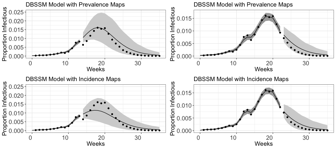
We perform two separate fits of this posterior model, on the first thirteen days () and on the first twenty two days (), for the considered ILI+ data for the 2010 influenza season in the United States. These fits are performed both using the original formulation of the DBSSM, which naively uses incidence data directly in place of prevalence data, and using the new formulation developed in this paper, which uses the new maps developed in Section 3 for a more principled treatment of incidence data. These fits and forecasts are outlined in Figure 2. The dark shaded grey regions prior to mark the 95 percentiles of the posterior density, while the lighter grey shaded regions after make the 95% prediction intervals. The forecast using incidence data up until has a narrower prediction interval than the one using prevalence data; each of the forecasts that use data up through are laregly comparable.
| Parameter | |||
|---|---|---|---|
| Prevalence Median | 2.15 | 1.60 | 1.21 |
| Incidence Median | 3.21 | 2.66 | 1.09 |

In addition to the slight improvements on forecasting we observe in Figure 2, this method also has strong implications for the interpretability of for the fitted model. Indeed, only the updated version of the DBSSM developed in this paper leads to realizations of these parameters that can accurately be interpreted as the infection rate (), recovery rate (), and the basic reproduction number ().
6 Discussion
The main contribution of this paper is the development of methods to map the time and value of peak incidence to the SIR curve parameters, and vice versa, for the purpose of forecasting tasks and inference on disease rate parameters. We do this by computationally solving a system of equations ((9) and (10)). There are several impactful uses of these maps in the context of previous literature. First, much like how the peak prevalence value (PPV) and time (PPT) are useful for public health response to an epidemic (Weiss, 2013), the analogous quantities for incidence are also useful, since they describe the influx new patients entering the hospital system on a given day. Second, this work improves upon existing work that uses historical prevalence data to model epidemics by creating a map from PIT and PIV to the SIR parameters, since incidence is typically the data that is available for ongoing epidemics (Osthus et al., 2017; Amaro, 2023). In the case of the application in Osthus et al. (2017), where incidence data were used in place of prevalence data without justification, we have shown that this leads to biased SIR parameter estimates (see Figure 3). Furthermore, our results indicate that forecasts performed using the erroneous data specification leads to larger prediction intervals earlier on in the outbreak, although this forecast is largely comparable for the correct specification later on in the outbreak (see Figure 2 and Remark 1). Of course, it remains more correct in principle to use incidence data appropriately when fitting compartment models for forecasting with ongoing incidence data (Nsoesie, Mararthe and Brownstein, 2013; Chowell et al., 2016; Abolmaali and Shirzaei, 2021). We have provided a modeling framework that incorporates this data appropriately (see Section 4). Lastly, while the methods discussed in McAndrew et al. (2024) do incorporate incidence data to fit forecasting models, this paper uses a Bayesian framework and importance sampling. Since the maps developed here are deterministic, they can be used in both a Bayesian and a Frequentist framework.
As a direction for future work, it would be useful to investigate better approximations for the solution to (13). The Taylor Approximation in Section 3.2.1 was by far the fastest computationally, but it came with the highest error on PIT. Finding a fast and accurate approximation to this equation would greatly increase the runtime for applications where the map between the SIR parameters and PIT/PIV must be evaluated several hundreds of thousands of times. However, for most applications (including the one in this paper), the Compute Integral approximation is sufficiently fast.
As a second direction for future work, it would be interesting to investigate the analogous maps for more complicated compartmental models, such as the SEIR model, the SIRS model, and the SEIRH model.
Open Research Section
All software used to perform the simulations and studies in this paper are publicly available at https://github.com/lanl/precog.
Acknowledgments
Research presented in this article was partially supported by the Laboratory Directed Research and Development program of Los Alamos National Laboratory under project number 20240066DR. Los Alamos National Laboratory is operated by Triad National Security, LLC, for the National Nuclear Security Administration of U.S. Department of Energy (Contract No. 89233218CNA000001).
This research was partially funded by NIH/NIGMS under grant R01GM130668-01 awarded to Sara Y. Del Valle.
Conflict of Interest
The authors have no non-financial or other financial competing interests to declare that are relevant to the content of this article other than the aforementioned declared funding sources.
References
- Abbey (1952) {barticle}[author] \bauthor\bsnmAbbey, \bfnmHelen\binitsH. (\byear1952). \btitleAN EXAMINATION OF THE REED-FROST THEORY OF EPIDEMICS. \bjournalHuman Biology \bvolume24 \bpages201–233. \endbibitem
- Abolmaali and Shirzaei (2021) {barticle}[author] \bauthor\bsnmAbolmaali, \bfnmSaina\binitsS. and \bauthor\bsnmShirzaei, \bfnmSamira\binitsS. (\byear2021). \btitleA comparative study of SIR Model, Linear Regression, Logistic Function and ARIMA Model for forecasting COVID-19 cases. \bjournalAIMS Public Health \bvolume8 \bpages598–613. \bdoi10.3934/publichealth.2021048 \endbibitem
- Acedo, González-Parra and Arenas (2010) {barticle}[author] \bauthor\bsnmAcedo, \bfnmL.\binitsL., \bauthor\bsnmGonzález-Parra, \bfnmGilberto\binitsG. and \bauthor\bsnmArenas, \bfnmAbraham J.\binitsA. J. (\byear2010). \btitleAn exact global solution for the classical SIRS epidemic model. \bjournalNonlinear Analysis: Real World Applications \bvolume11 \bpages1819-1825. \bdoihttps://doi.org/10.1016/j.nonrwa.2009.04.007 \endbibitem
- Amaro (2023) {barticle}[author] \bauthor\bsnmAmaro, \bfnmJ. E.\binitsJ. E. (\byear2023). \btitleSystematic description of COVID-19 pandemic using exact SIR solutions and Gumbel distributions. \bjournalNonlinear Dynamics \bvolume111 \bpages1947–1969. \bdoi10.1007/s11071-022-07907-4 \endbibitem
- Anderson (1988) {barticle}[author] \bauthor\bsnmAnderson, \bfnmRoy M\binitsR. M. (\byear1988). \btitleThe role of mathematical models in the study of HIV transmission and the epidemiology of AIDS. \bjournalJournal of Acquired Immune Deficiency Syndromes \bvolume1 \bpages241–256. \endbibitem
- Bailey (1957) {bbook}[author] \bauthor\bsnmBailey, \bfnmNorman T. J.\binitsN. T. J. (\byear1957). \btitleThe mathematical theory of epidemics. \bpublisherGriffin. \endbibitem
- Cadoni and Gaeta (2020) {barticle}[author] \bauthor\bsnmCadoni, \bfnmMariano\binitsM. and \bauthor\bsnmGaeta, \bfnmGiuseppe\binitsG. (\byear2020). \btitleSize and timescale of epidemics in the SIR framework. \bjournalPhysica D: Nonlinear Phenomena \bvolume411 \bpages132626. \bdoihttps://doi.org/10.1016/j.physd.2020.132626 \endbibitem
- Carvalho and Gonçalves (2021) {barticle}[author] \bauthor\bsnmCarvalho, \bfnmAlexsandro M.\binitsA. M. and \bauthor\bsnmGonçalves, \bfnmSebastián\binitsS. (\byear2021). \btitleAn analytical solution for the Kermack–McKendrick model. \bjournalPhysica A: Statistical Mechanics and its Applications \bvolume566 \bpages125659. \bdoihttps://doi.org/10.1016/j.physa.2020.125659 \endbibitem
- Castro et al. (2020) {barticle}[author] \bauthor\bsnmCastro, \bfnmMario\binitsM., \bauthor\bsnmAres, \bfnmSaúl\binitsS., \bauthor\bsnmCuesta, \bfnmJosé A.\binitsJ. A. and \bauthor\bsnmManrubia, \bfnmSusanna\binitsS. (\byear2020). \btitleThe turning point and end of an expanding epidemic cannot be precisely forecast. \bjournalProceedings of the National Academy of Sciences \bvolume117 \bpages26190-26196. \bdoi10.1073/pnas.2007868117 \endbibitem
- CDC (2023) {bmisc}[author] \bauthor\bsnmCDC, (\byear2023). \btitleU.S. Influenza Surveillance: Purpose and Methods. \bnotedata retrieved from Centers for Disease Control and Prevention, National Center for Immunization and Respiratory Diseases (NCIRD), https://www.cdc.gov/flu/weekly/overview.htm. \endbibitem
- CDC (2024) {bmisc}[author] \bauthor\bsnmCDC, (\byear2024). \btitleGlossary of Influenza (Flu) Terms. \bnotedata retrieved from Centers for Disease Control and Prevention, National Center for Immunization and Respiratory Diseases (NCIRD), https://www.cdc.gov/flu/about. \endbibitem
- Chowell et al. (2016) {barticle}[author] \bauthor\bsnmChowell, \bfnmGerardo\binitsG., \bauthor\bsnmSattenspiel, \bfnmLisa\binitsL., \bauthor\bsnmBansal, \bfnmShweta\binitsS. and \bauthor\bsnmViboud, \bfnmCécile\binitsC. (\byear2016). \btitleMathematical models to characterize early epidemic growth: A review. \bjournalPhys Life Rev \bvolume18 \bpages66–97. \bdoi10.1016/j.plrev.2016.07.005 \endbibitem
- Chretien, Riley and George (2015) {barticle}[author] \bauthor\bsnmChretien, \bfnmJean-Paul\binitsJ.-P., \bauthor\bsnmRiley, \bfnmSteven\binitsS. and \bauthor\bsnmGeorge, \bfnmDylan B\binitsD. B. (\byear2015). \btitleMathematical modeling of the West Africa Ebola epidemic. \bjournalElife \bvolume4 \bpagese09186. \endbibitem
- Cooper, Mondal and Antonopoulos (2020) {barticle}[author] \bauthor\bsnmCooper, \bfnmIan\binitsI., \bauthor\bsnmMondal, \bfnmArgha\binitsA. and \bauthor\bsnmAntonopoulos, \bfnmChris G\binitsC. G. (\byear2020). \btitleA SIR model assumption for the spread of COVID-19 in different communities. \bjournalChaos Solitons Fractals \bvolume139 \bpages110057. \bdoi10.1016/j.chaos.2020.110057 \endbibitem
- Deakin (1975) {barticle}[author] \bauthor\bsnmDeakin, \bfnmMichael A. B.\binitsM. A. B. (\byear1975). \btitleA standard form for the Kermack-McKendrick epidemic equations. \bjournalBulletin of Mathematical Biology \bvolume37 \bpages91-95. \bdoihttps://doi.org/10.1016/S0092-8240(75)80011-5 \endbibitem
- Golub, Gorr and Gould (1993) {barticle}[author] \bauthor\bsnmGolub, \bfnmAndrew\binitsA., \bauthor\bsnmGorr, \bfnmWilpen L\binitsW. L. and \bauthor\bsnmGould, \bfnmPeter R\binitsP. R. (\byear1993). \btitleSpatial diffusion of the HIV/AIDS epidemic: modeling implications and case study of AIDS incidence in Ohio. \bjournalGeographical analysis \bvolume25 \bpages85–100. \endbibitem
- Guanghong et al. (2004) {barticle}[author] \bauthor\bsnmGuanghong, \bfnmDing\binitsD., \bauthor\bsnmChang, \bfnmLiu\binitsL., \bauthor\bsnmJianqiu, \bfnmGong\binitsG., \bauthor\bsnmLing, \bfnmWang\binitsW., \bauthor\bsnmKe, \bfnmCheng\binitsC. and \bauthor\bsnmDi, \bfnmZhang\binitsZ. (\byear2004). \btitleSARS epidemical forecast research in mathematical model. \bjournalChinese Science Bulletin \bvolume49 \bpages2332–2338. \endbibitem
- Harko, Lobo and Mak (2014) {barticle}[author] \bauthor\bsnmHarko, \bfnmTiberiu\binitsT., \bauthor\bsnmLobo, \bfnmFrancisco S. N.\binitsF. S. N. and \bauthor\bsnmMak, \bfnmM. K.\binitsM. K. (\byear2014). \btitleExact analytical solutions of the Susceptible-Infected-Recovered (SIR) epidemic model and of the SIR model with equal death and birth rates. \bjournalApplied Mathematics and Computation \bvolume236 \bpages184-194. \bdoihttps://doi.org/10.1016/j.amc.2014.03.030 \endbibitem
- Hethcote (1976) {barticle}[author] \bauthor\bsnmHethcote, \bfnmHerbert W.\binitsH. W. (\byear1976). \btitleQualitative analyses of communicable disease models. \bjournalMathematical Biosciences \bvolume28 \bpages335-356. \bdoihttps://doi.org/10.1016/0025-5564(76)90132-2 \endbibitem
- Hethcote (2000) {barticle}[author] \bauthor\bsnmHethcote, \bfnmHerbert W\binitsH. W. (\byear2000). \btitleThe mathematics of infectious diseases. \bjournalSIAM review \bvolume42 \bpages599–653. \endbibitem
- Kendall (1956) {binproceedings}[author] \bauthor\bsnmKendall, \bfnmDavid G\binitsD. G. (\byear1956). \btitleDeterministic and stochastic epidemics in closed populations. In \bbooktitleProceedings of the third Berkeley symposium on mathematical statistics and probability \bvolume4 \bpages149–165. \bpublisherUniversity of California Press Berkeley. \endbibitem
- Kermack, McKendrick and Walker (1927) {barticle}[author] \bauthor\bsnmKermack, \bfnmWilliam Ogilvy\binitsW. O., \bauthor\bsnmMcKendrick, \bfnmA. G.\binitsA. G. and \bauthor\bsnmWalker, \bfnmGilbert Thomas\binitsG. T. (\byear1927). \btitleA contribution to the mathematical theory of epidemics. \bjournalProceedings of the Royal Society of London. Series A, Containing Papers of a Mathematical and Physical Character \bvolume115 \bpages700-721. \bdoi10.1098/rspa.1927.0118 \endbibitem
- Kröger, Turkyilmazoglu and Schlickeiser (2021) {barticle}[author] \bauthor\bsnmKröger, \bfnmMartin\binitsM., \bauthor\bsnmTurkyilmazoglu, \bfnmMustafa\binitsM. and \bauthor\bsnmSchlickeiser, \bfnmReinhard\binitsR. (\byear2021). \btitleExplicit formulae for the peak time of an epidemic from the SIR model. Which approximant to use? \bjournalPhysica D: Nonlinear Phenomena \bvolume425 \bpages132981. \bdoihttps://doi.org/10.1016/j.physd.2021.132981 \endbibitem
- LaDeau et al. (2011) {barticle}[author] \bauthor\bsnmLaDeau, \bfnmShannon L\binitsS. L., \bauthor\bsnmGlass, \bfnmGregory E\binitsG. E., \bauthor\bsnmHobbs, \bfnmN Thompson\binitsN. T., \bauthor\bsnmLatimer, \bfnmAndrew\binitsA. and \bauthor\bsnmOstfeld, \bfnmRichard S\binitsR. S. (\byear2011). \btitleData–model fusion to better understand emerging pathogens and improve infectious disease forecasting. \bjournalEcological Applications \bvolume21 \bpages1443–1460. \endbibitem
- Lang et al. (2018) {barticle}[author] \bauthor\bsnmLang, \bfnmJohn C\binitsJ. C., \bauthor\bsnmDe Sterck, \bfnmHans\binitsH., \bauthor\bsnmKaiser, \bfnmJamieson L\binitsJ. L. and \bauthor\bsnmMiller, \bfnmJoel C\binitsJ. C. (\byear2018). \btitleAnalytic models for SIR disease spread on random spatial networks. \bjournalJournal of Complex Networks \bvolume6 \bpages948-970. \bdoi10.1093/comnet/cny004 \endbibitem
- Massad et al. (2005) {barticle}[author] \bauthor\bsnmMassad, \bfnmEduardo\binitsE., \bauthor\bsnmBurattini, \bfnmMarcelo N\binitsM. N., \bauthor\bsnmLopez, \bfnmLuis F\binitsL. F. and \bauthor\bsnmCoutinho, \bfnmFrancisco A B\binitsF. A. B. (\byear2005). \btitleForecasting versus projection models in epidemiology: the case of the SARS epidemics. \bjournalMed Hypotheses \bvolume65 \bpages17–22. \bdoi10.1016/j.mehy.2004.09.029 \endbibitem
- McAndrew et al. (2024) {barticle}[author] \bauthor\bsnmMcAndrew, \bfnmThomas\binitsT., \bauthor\bsnmGibson, \bfnmGraham C.\binitsG. C., \bauthor\bsnmBraun, \bfnmDavid\binitsD., \bauthor\bsnmSrivastava, \bfnmAbhishek\binitsA. and \bauthor\bsnmBrown, \bfnmKate\binitsK. (\byear2024). \btitleChimeric Forecasting: An experiment to leverage human judgment to improve forecasts of infectious disease using simulated surveillance data. \bjournalEpidemics \bvolume47 \bpages100756. \bdoihttps://doi.org/10.1016/j.epidem.2024.100756 \endbibitem
- Miller (2009) {barticle}[author] \bauthor\bsnmMiller, \bfnmJoel C\binitsJ. C. (\byear2009). \btitleSpread of infectious disease through clustered populations. \bjournalJ R Soc Interface \bvolume6 \bpages1121–1134. \bdoi10.1098/rsif.2008.0524 \endbibitem
- Murray (2002) {bbook}[author] \bauthor\bsnmMurray, \bfnmJames Dickson\binitsJ. D. (\byear2002). \btitleMathematical Biology: An introduction. \bpublisherSpringer. \endbibitem
- Noordzij et al. (2010) {barticle}[author] \bauthor\bsnmNoordzij, \bfnmMarlies\binitsM., \bauthor\bsnmDekker, \bfnmFriedo W\binitsF. W., \bauthor\bsnmZoccali, \bfnmCarmine\binitsC. and \bauthor\bsnmJager, \bfnmKitty J\binitsK. J. (\byear2010). \btitleMeasures of disease frequency: prevalence and incidence. \bjournalNephron Clin Pract \bvolume115 \bpagesc17-20. \bdoi10.1159/000286345 \endbibitem
- Nsoesie, Mararthe and Brownstein (2013) {barticle}[author] \bauthor\bsnmNsoesie, \bfnmElaine\binitsE., \bauthor\bsnmMararthe, \bfnmMadhav\binitsM. and \bauthor\bsnmBrownstein, \bfnmJohn\binitsJ. (\byear2013). \btitleForecasting peaks of seasonal influenza epidemics. \bjournalPLoS Curr \bvolume5. \bdoi10.1371/currents.outbreaks.bb1e879a23137022ea79a8c508b030bc \endbibitem
- Nsoesie et al. (2014) {barticle}[author] \bauthor\bsnmNsoesie, \bfnmElaine O\binitsE. O., \bauthor\bsnmBrownstein, \bfnmJohn S\binitsJ. S., \bauthor\bsnmRamakrishnan, \bfnmNaren\binitsN. and \bauthor\bsnmMarathe, \bfnmMadhav V\binitsM. V. (\byear2014). \btitleA systematic review of studies on forecasting the dynamics of influenza outbreaks. \bjournalInfluenza and other respiratory viruses \bvolume8 \bpages309–316. \endbibitem
- Nyabadza, Mukandavire and Hove-Musekwa (2011) {barticle}[author] \bauthor\bsnmNyabadza, \bfnmF.\binitsF., \bauthor\bsnmMukandavire, \bfnmZ.\binitsZ. and \bauthor\bsnmHove-Musekwa, \bfnmS. D.\binitsS. D. (\byear2011). \btitleModelling the HIV/AIDS epidemic trends in South Africa: Insights from a simple mathematical model. \bjournalNonlinear Analysis: Real World Applications \bvolume12 \bpages2091-2104. \bdoihttps://doi.org/10.1016/j.nonrwa.2010.12.024 \endbibitem
- Osthus et al. (2017) {barticle}[author] \bauthor\bsnmOsthus, \bfnmDave\binitsD., \bauthor\bsnmHickmann, \bfnmKyle S\binitsK. S., \bauthor\bsnmCaragea, \bfnmPetruţa C\binitsP. C., \bauthor\bsnmHigdon, \bfnmDave\binitsD. and \bauthor\bsnmDel Valle, \bfnmSara Y\binitsS. Y. (\byear2017). \btitleForecasting seasonal influenza with a state-space SIR model. \bjournalAnn Appl Stat \bvolume11 \bpages202–224. \bdoi10.1214/16-AOAS1000 \endbibitem
- Osthus et al. (2019) {barticle}[author] \bauthor\bsnmOsthus, \bfnmDave\binitsD., \bauthor\bsnmGattiker, \bfnmJames\binitsJ., \bauthor\bsnmPriedhorsky, \bfnmReid\binitsR. and \bauthor\bsnmValle, \bfnmSara Y. Del\binitsS. Y. D. (\byear2019). \btitleDynamic Bayesian Influenza Forecasting in the United States with Hierarchical Discrepancy (with Discussion). \bjournalBayesian Analysis \bvolume14 \bpages261 – 312. \bdoi10.1214/18-BA1117 \endbibitem
- Piovella (2020) {barticle}[author] \bauthor\bsnmPiovella, \bfnmNicola\binitsN. (\byear2020). \btitleAnalytical solution of SEIR model describing the free spread of the COVID-19 pandemic. \bjournalChaos, Solitons & Fractals \bvolume140 \bpages110243. \bdoihttps://doi.org/10.1016/j.chaos.2020.110243 \endbibitem
- Prangle (2016) {barticle}[author] \bauthor\bsnmPrangle, \bfnmDennis\binitsD. (\byear2016). \btitleLazy ABC. \bjournalStatistics and Computing \bvolume26 \bpages171–185. \bdoi10.1007/s11222-014-9544-3 \endbibitem
- Schlickeiser and Kröger (2021) {barticle}[author] \bauthor\bsnmSchlickeiser, \bfnmR\binitsR. and \bauthor\bsnmKröger, \bfnmM\binitsM. (\byear2021). \btitleAnalytical solution of the SIR-model for the temporal evolution of epidemics: part B. Semi-time case. \bjournalJournal of Physics A: Mathematical and Theoretical \bvolume54 \bpages175601. \bdoi10.1088/1751-8121/abed66 \endbibitem
- Shaman et al. (2013) {barticle}[author] \bauthor\bsnmShaman, \bfnmJeffrey\binitsJ., \bauthor\bsnmKarspeck, \bfnmAlicia\binitsA., \bauthor\bsnmYang, \bfnmWan\binitsW., \bauthor\bsnmTamerius, \bfnmJames\binitsJ. and \bauthor\bsnmLipsitch, \bfnmMarc\binitsM. (\byear2013). \btitleReal-time influenza forecasts during the 2012–2013 season. \bjournalNature communications \bvolume4 \bpages2837. \endbibitem
- Turkyilmazoglu (2021) {barticle}[author] \bauthor\bsnmTurkyilmazoglu, \bfnmMustafa\binitsM. (\byear2021). \btitleExplicit formulae for the peak time of an epidemic from the SIR model. \bjournalPhysica D: Nonlinear Phenomena \bvolume422 \bpages132902. \bdoihttps://doi.org/10.1016/j.physd.2021.132902 \endbibitem
- Walter and Contreras (1999) {binbook}[author] \bauthor\bsnmWalter, \bfnmGilbert G.\binitsG. G. and \bauthor\bsnmContreras, \bfnmMartha\binitsM. (\byear1999). \btitleIntroduction to Compartmental Models \bpages111–123. \bpublisherBirkhäuser Boston, \baddressBoston, MA. \bdoi10.1007/978-1-4612-1590-5_13 \endbibitem
- Wang, Wei and Zhang (2014) {barticle}[author] \bauthor\bsnmWang, \bfnmXiaoyun\binitsX., \bauthor\bsnmWei, \bfnmLijuan\binitsL. and \bauthor\bsnmZhang, \bfnmJuan\binitsJ. (\byear2014). \btitleDynamical analysis and perturbation solution of an SEIR epidemic model. \bjournalApplied Mathematics and Computation \bvolume232 \bpages479-486. \bdoihttps://doi.org/10.1016/j.amc.2014.01.090 \endbibitem
- Weiss (2013) {barticle}[author] \bauthor\bsnmWeiss, \bfnmHoward Howie\binitsH. H. (\byear2013). \btitleThe SIR model and the foundations of public health. \bjournalMaterials matematics \bpages0001–17. \endbibitem
- Zhan et al. (2019) {barticle}[author] \bauthor\bsnmZhan, \bfnmZhicheng\binitsZ., \bauthor\bsnmDong, \bfnmWeihua\binitsW., \bauthor\bsnmLu, \bfnmYongmei\binitsY., \bauthor\bsnmYang, \bfnmPeng\binitsP., \bauthor\bsnmWang, \bfnmQuanyi\binitsQ. and \bauthor\bsnmJia, \bfnmPeng\binitsP. (\byear2019). \btitleReal-Time Forecasting of Hand-Foot-and-Mouth Disease Outbreaks using the Integrating Compartment Model and Assimilation Filtering. \bjournalScientific Reports \bvolume9 \bpages2661. \bdoi10.1038/s41598-019-38930-y \endbibitem
- Zhang et al. (2022) {barticle}[author] \bauthor\bsnmZhang, \bfnmPeijue\binitsP., \bauthor\bsnmFeng, \bfnmKairui\binitsK., \bauthor\bsnmGong, \bfnmYuqing\binitsY., \bauthor\bsnmLee, \bfnmJieon\binitsJ., \bauthor\bsnmLomonaco, \bfnmSara\binitsS. and \bauthor\bsnmZhao, \bfnmLiang\binitsL. (\byear2022). \btitleUsage of Compartmental Models in Predicting COVID-19 Outbreaks. \bjournalThe AAPS Journal \bvolume24 \bpages98. \bdoi10.1208/s12248-022-00743-9 \endbibitem
- Zhao and Chen (2020) {barticle}[author] \bauthor\bsnmZhao, \bfnmShilei\binitsS. and \bauthor\bsnmChen, \bfnmHua\binitsH. (\byear2020). \btitleModeling the epidemic dynamics and control of COVID-19 outbreak in China. \bjournalQuantitative Biology \bvolume8 \bpages11-19. \bdoihttps://doi.org/10.1007/s40484-020-0199-0 \endbibitem
Appendix A Specification of the Dirichlet-Beta State-Space Model
The DBSSM is fit using a fully Bayesian framework, where the interest lies in estimating the joint posterior density of the latent space and given the observed data . Using the conditional independence assumption described above, this density can be written as follows:
| (27) |
where is some prior on , is the data likelihood determined by (17), and the distribution is determined by (18). To perform forecasts on observations , where is the final timepoint of the outbreak, one uses the posterior predictive distribution, where the model and latent-space parameters are integrated out:
| (28) |
To complete the specification of the DBSSM, one must determine what priors to put on the model parameters in . It is here that the authors in Osthus et al. (2017) directly address the aforementioned stability issues with fitting an SIR curve with early pandemic data. Define the latent variable , and let be the expanded model parameter vector that includes . We factorize the new prior distribution on to get
| (29) |
Several modeling assumptions on this conditional distribution give the abbreviated form,
| (30) |
Specification of the individual distributions in (30) is what remains to fully define the DBSSM. The priors and remain unchanged and can be found in the original paper. In Section 4, the priors on and are described and updated, when necessary, with the theory developed in this paper.