2024
[1]\fnmQuanying \surLiu
1]\orgdivDepartment of Biomedical Engineering, \orgnameSouthern University of Science and Technology, \orgaddress\cityShenzhen, \postcode518055, \countryChina
2]\orgdivDepartment of Electrical and Computer Engineering, \orgnameIowa State University, \orgaddress\cityAmes, \postcode50011, \stateIowa, \countryUSA
3]\orgdivDepartment of Mathematics and Division of Life Science, \orgnameThe Hong Kong University of Science and Technology, \orgaddress\streetHong Kong SAR, \countryChina
4]\orgdivDepartment of Physics, Centre for Nonlinear Studies, \orgnameHong Kong Baptist University, \orgaddress\streetHong Kong SAR, \countryChina
Mapping effective connectivity by virtually perturbing a surrogate brain
Abstract
Effective connectivity (EC), indicative of the causal interactions between brain regions, is fundamental to understanding information processing in the brain. Traditional approaches, which infer EC from neural responses to stimulations, are not suited for mapping whole-brain EC in humans due to being invasive and having limited spatial coverage of stimulations. To address this gap, we present Neural Perturbational Inference (NPI), a data-driven framework designed to map EC across the entire brain. NPI employs an artificial neural network trained to learn large-scale neural dynamics as a computational surrogate of the brain. NPI maps EC by perturbing each region of the surrogate brain and observing the resulting responses in all other regions. NPI captures the directionality, strength, and excitatory/inhibitory properties of brain-wide EC. Our validation of NPI, using models having ground-truth EC, shows its superiority over Granger causality and dynamic causal modeling. Applying NPI to resting-state fMRI data from diverse datasets reveals consistent and structurally supported EC. Further validation using a cortico-cortical evoked potentials dataset reveals a significant correlation between NPI-inferred EC and real stimulation propagation pathways. By transitioning from correlational to causal understandings of brain functionality, NPI marks a stride in decoding the brain’s functional architecture and facilitating both neuroscience research and clinical applications.
1 Introduction
The brain operates as an intricate network of interconnected regions, which collaboratively processes external stimuli to generate behavior Park2013Structural ; deco2021revisiting . Understanding the information flow between these regions is key to deciphering brain function Park2013Structural ; seguin2023brain . While structural connectivity (SC) maps the brain’s physical wiring and functional connectivity (FC) identifies statistical dependencies among neural activities, these measures fall short of illustrating the directional flow of information Yeh2021Mapping ; vandenHeuvel2010Exploring . Effective connectivity (EC), delineating the causal interactions between brain regions, is thus essential for understanding information flow and critical in selecting target nodes for neuromodulation in brain disorder treatments Schippers2010Mapping ; manjunatha2024controlling .
EC is traditionally derived through neurostimulation experiments, such as optogenetics Kim2023Wholebrain ; Randi2023Neural or deep brain stimulation (DBS) Hollunder2024Mapping . These methods involve perturbing specific brain regions and monitoring the resultant neural responses in other areas, thereby providing direct evidence of causality. However, such ‘perturbing and recording’ procedures are invasive and do not scale well for whole-brain analysis. Computational approaches offer non-invasive alternatives but often suffer from inaccuracies, especially when applied at a whole-brain scale. Model-based methods, like Dynamic causal modeling (DCM), heavily rely on underlying model assumptions and are prone to biases from model mismatches Friston2014DCM . On the other hand, model-free methods such as Granger causality (GC) are adept at discerning the directionality of EC but struggle to accurately measure its strength or differentiate between excitatory and inhibitory influences Li2018Causal . Moreover, the interpretation of EC varies across computational frameworks, leading to ambiguity in the interpretation of EC inferred from computational and experimental approaches.
The advent of big data in neuroscience, propelled by advanced imaging and electrophysiological techniques, has facilitated the use of artificial neural networks (ANN) to analyze complex neural data Liang2022Online ; abrol2021deep . Recurrent neural network models have been employed to learn temporal dynamics of brain signals and infer EC directly from the learned weight matrices Perich2020Inferring ; tu2019state . While these models can capture brain dynamics, there is no guarantee that the learned weights reflect the underlying EC, particularly when the model’s assumptions do not align with the brain’s underlying dynamics and when dealing with a large number of regions Das2020Systematic . Perturbation analysis in ANN presents a promising avenue for investigating causality, where modulating input variables and observing subsequent output changes allow for the elucidation of causal relationships tied to specific inputs and their effects ivanovs2021perturbation ; dong2023causal . Such perturbational approaches are conceptually similar to using stimulation-evoked potentials to infer EC in neuroscience, aiming to delineate causal connections Veit2021Temporal ; Ozdemir2020Individualized . Inspired by this parallel, our study integrates perturbation-based experiments into a data-driven framework, revealing the brain causality at a whole-brain level.
In this study, we present the Neural Perturbational Inference (NPI) technique for non-invasively mapping whole-brain EC. NPI utilizes an ANN that learns the brain dynamics as a surrogate brain. After the ANN is well-trained to capture the brain-wide neural dynamics, systematically perturbing the trained ANN yields a map of causal relationships among all brain regions. It delineates the directionality, strength, and excitatory/inhibitory properties of whole-brain causal interactions. The effectiveness of NPI is validated on a variety of generative models with established ground-truth EC. NPI shows a remarkable match with cortico-cortical evoked potentials, validating its accuracy in reflecting real causal interactions in the brain. NPI holds promise for advancing the understanding of brain information flow and the clinical treatment of neurological disorders.

2 Results
2.1 Neural Perturbational Inference
NPI is a framework that non-invasively infers EC from neural signals (Fig. 1a-d). Conceptually, NPI is similar to perturbing the real brain through neurostimulation, but it uses an ANN as a surrogate brain to replace the real brain, which enables efficient whole-brain perturbation and observation.
From brain imaging or electrophysiological recordings, the collective neural activities of multiple brain regions are easily available, but how these regions interact to process information is unclear (Fig. 1a). NPI aims to infer EC among regions for the entire brain, which are directed causal connections. This study implemented the ANN as a multi-layer perceptron (MLP; Supplementary Fig. 1). The ANN in NPI can be implemented as different predictive models as long as the model can learn brain dynamics and capture inter-region relationships (Supplementary Fig. 2, Supplementary Note 1,2). In addition to the MLP network, we tested various surrogate models (e.g., CNN, RNN, VAR) to assess their performance in signal prediction, FC reproduction, and EC inference (Supplementary Table 1). The results show that the NPI framework remains robust across different ANN architectures. The ANN is trained to predict the brain state at the next time step based on the brain states of the preceding three time steps by minimizing the one-step-ahead prediction error (Fig. 1b). To validate the ability of ANN to capture the interaction relationships between brain regions. We recursively fed the predicted output into the ANN and generated the synthetic signals (Fig. 1e). On human BOLD data, the FC calculated from the synthetic BOLD signals (model FC) and the empirical BOLD signals (empirical FC) are compared, both of which are averaged across 800 subjects in the HCP dataset. The model FC and empirical FC are strongly correlated (, ), suggesting ANN captures complex inter-region relationship in the brain, which is crucial for the EC inference (Fig. 1f). This suggests that the trained ANN can serve as a surrogate brain for virtual perturbations.
The trained ANN is fixed and treated as a surrogate model for the brain. We then applied virtual perturbations to each node of the ANN, with each node representing a brain region (Fig. 1c). The perturbation is implemented as an impulse increase to the signal at the selected node at time (Fig. 1g). The ANN takes both perturbed input and baseline input to predict subsequent neural activities . Changes in the predicted responses of target regions — when comparing perturbed input to baseline input — reflect the EC from the source region (the perturbed region) to the target regions. Increased or decreased activity in the target regions indicates excitatory or inhibitory EC, respectively (Fig. 1h). Systematically perturbing each node in the ANN reveals the all-to-all EC (Fig. 1d), characterizing the directionality, strength, and excitatory/inhibitory properties of causal influences among brain regions. We show that this systematic perturbation is interpreted as the Jacobian matrix of the trained ANN (Supplementary Note 4, Extended Data Fig. 2), which quantifies how a small input to one node can positively or negatively influence the next states of other nodes.
To validate the effectiveness of NPI, we applied it to data generated by pre-defined generative models with established ground-truth EC (Fig. 1i). We quantify the EC inference performance by comparing the NPI-inferred EC with the ground-truth EC. When applied to real rs-fMRI datasets, NPI can reveal seed-based EC and the whole-brain EC, uncovering the distribution of EC both within and across functional brain networks (Fig. 1j).
2.2 Validation of NPI on generative models

We first validated the capability of NPI by applying it to infer EC from synthetic data generated by models with established ground-truth EC (see Methods). We used three simulated datasets: synthetic data generated by ground-truth recurrent neural network (RNN) models, a public synthetic BOLD dataset with few brain regions, and synthetic BOLD data using a whole brain model (WBM). To derive the ground-truth EC, we used the ’perturb and record’ protocol directly on the generative models. We assessed NPI’s inference performance by comparing this ground-truth EC with the EC inferred by NPI.
NPI was firstly applied to infer EC from a RNN with a pre-defined weight matrix serving as SC, where the entries were drawn from a Gaussian distribution centered at zero (Fig. 2a). The neural signals are then synthesized by executing the RNN (Fig. 2b). An ANN is fitted to the signals generated by the RNN as a surrogate. The ANN’s ability to learn the non-linear RNN system dynamics is evidenced by its successful generation of synthetic signals when its output is recursively fed back into the system (Fig. 2c). FC derived from the ANN-synthesized signals demonstrated a strong correlation with FC directly calculated from the RNN-generated signals, implying ANN’s proficiency in capturing the RNN’s inter-regional dynamics (Fig. 2d).
To derive EC, perturbations are then applied to the trained ANN (Fig. 2e, Supplementary Fig. 2,3). The RNN’s intrinsic EC, obtained through perturbing the ground-truth RNN directly, is used as ground-truth EC (Fig. 2f). We calculated the correlation between NPI-inferred EC and ground-truth EC, as well as the correlation between GC-inferred EC and ground-truth EC (Supplementary Note 5). The results show a strong alignment between NPI-inferred EC and the ground-truth EC, with correlation coefficient of , outperforming GC (Fig. 2g, Supplementary Fig. 4). The NPI-inferred EC also demonstrates a strong correlation with the SC of RNN, which serves as the anatomical foundation for EC (Supplementary Fig. 4). EC does not perfectly align with SC due to the inherent nonlinearity of brain dynamics and signal noise, the correlation between EC and SC is significantly stronger than that between FC and SC (Supplementary Table 2). This is likely because FC lacks directionality and suffers from spurious connectivity power2012spurious . To evaluate the robustness of the NPI, we conducted comprehensive analyses, including applying a range of perturbation intensities to the ANN, varying levels of systemic noise to the RNN model, and varying data lengths and RNN sizes (Fig. 2h). The results showed that NPI’s EC inference performance remains stable across different perturbation magnitudes and experiences only a slight decline with increasing noise levels, demonstrating the method’s robustness. In scenarios with varying data lengths and RNN sizes, we found that larger datasets are crucial for reliable EC inference on larger networks.
To examine the NPI’s efficacy on BOLD signals and on networks with different structures, we applied NPI to a public synthetic dataset containing BOLD dynamics generated from nine different underlying SC structures Sanchez-Romero2019Estimating (Fig. 2i, Extended Data Fig. 3a). This dataset, widely used in validating EC inference algorithms, features binary SC and simulates neural firing rates subsequently converted into BOLD signals through a hemodynamic response function (see Methods). For this dataset, as the ground-truth EC is unavailable, we evaluated the performance of EC inference using the Area Under the Receiver Operating Characteristic Curve (AUC) by classifying the presence or absence of each possible SC connection after binarizing the NPI-inferred EC. We show that NPI achieved an AUC close to 1, surpassing GC and DCM (Fig. 2j). Across all nine SC configurations, NPI significantly outperformed both GC and DCM (Extended Data Fig. 3), demonstrating its precision and reliability in mapping EC across diverse connection topographies and model structures.
Inferring EC from a large-scale network poses challenges for conventional methods like DCM. To validate NPI’s effectiveness in large-scale EC inference, we applied NPI to the synthetic BOLD data generated from a whole-brain model (WBM) with 66 nodes (see Methods). Specifically, we utilized neuroanatomical connectivity data obtained via Diffusion Spectrum Imaging (DSI) as the underlying SC matrix. The BOLD time series were then generated by a neurodynamic model (Fig. 2k). Despite a decline in multi-step prediction accuracy (Fig. 2l, Supplementary Fig. 7), the FC of the ANN-generated signals shows a strong correlation with the FC of the WBM-simulated signals (Fig. 2m), highlighting the ANN’s effectiveness in capturing the inter-regional relationships. Ground-truth EC from the WBM was obtained by perturbing each node and observing the resulting responses. The NPI-inferred EC not only shows a strong correlation with the ground-truth EC but also closely aligns with the underlying SC (Fig. 2n, Supplementary Fig. 5,6). Furthermore, NPI-inferred EC more accurately reflects both the ground-truth EC and SC compared to EC inferred by GC (Fig. 2o,p, , Wilcoxon signed-rank test), establishing NPI as a robust and reliable method for EC estimation in complex brain networks. On this dataset, we tested the performance of different surrogate models and found MLP gives the best FC reproduction and EC inference performance (Supplementary Tables 1, and 2). We thus use the MLP to be the surrogate model for inferring EC from real data.
2.3 Human EBC inferred by NPI
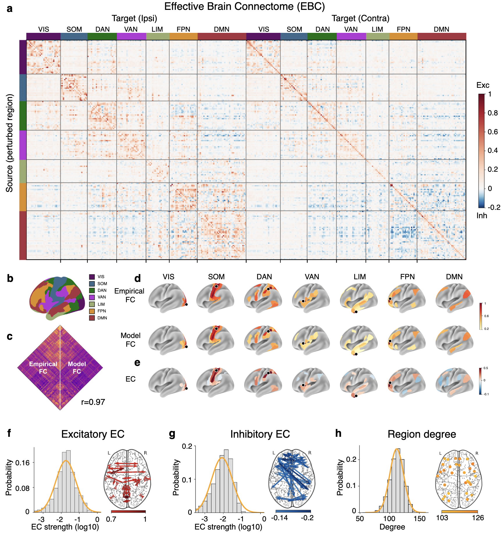
We applied NPI to resting-state fMRI (rs-fMRI) data from 800 subjects in the Human Connectome Project (HCP) dataset parcellated using the Multi-Modal Parcellation atlas with 360 regions (Supplementary Table 5) VanEssen2013WUMinn ; Glasser2016Multimodal . The individualized ANN was trained on the rs-fMRI data of each subject (see Methods). Using the signals from the previous three steps to predict the next step yielded slightly better performance compared to using only the signals from the previous step as input (Supplementary Fig. 8). Therefore, we used the 3-step input MLP model for the following analysis. The trained ANN can be treated as an individualized surrogate model. The group-level FC calculated from the real BOLD signals (i.e., empirical FC) and the ANN-generated BOLD signals (i.e., model FC) have a strong positive correlation (r=0.97, Fig. 3c) and share similar spatial patterns (Fig. 3d), suggesting that the trained ANN captures the complex inter-regional interactions of the biological brain.
After the surrogate model was trained, we applied systematic perturbations to each individualized surrogate model to obtain the whole-brain EC, which we call the effective brain connectome (EBC). We first obtained the individualized EBC by perturbing the individualized surrogate model and then calculated the group-level EBC (i.e., Human EBC) by averaging the EBC across 800 subjects (Fig. 3a). The positive entries indicate excitatory EC and negative entries indicate inhibitory EC. The brain regions are assigned to seven functional networks (i.e., visual network (VIS), somatomotor network (SOM), dorsal attention network (DAN), ventral attention network (VAN), limbic network (LIM), frontoparietal network (FPN), and default mode network (DMN)) according to Yeo et al. ThomasYeo2011organization (Supplementary Table 3, Fig. 3b). Seed-based EC is then analyzed to examine the topographic organization of functional networks. The top 10% excitatory and top 10% inhibitory output EC from seeds in six functional brain networks are plotted, showing a similar structure as networks defined by FC and better reflects how seed regions inhibit other parts across the whole brain (Fig. 3e).
The majority of EC have small and near-zero strengths, with a few having very large strengths. The distribution shows a long-tail property. We fit the strengths to four hypothesized distributions: log-normal, normal, exponential, and inverse Gaussian. According to the Akaike information criterion (AIC), the log-normal distribution is the best fit for both excitatory and inhibitory EC (Fig. 3f,g, Supplementary Table 4). It is consistent with the distribution of SC found in experimental studies using tract-tracing techniques involving mice and macaques Oh2014mesoscale ; Markov2014Weighted . The log-normal distributions of excitatory and inhibitory EC are reproducible under the Automated Anatomical Labeling (AAL) parcellation (Supplementary Fig. 9). The excitatory EC has stronger strength than inhibitory EC. When the maximum strength of excitatory EC is scaled to 1, inhibitory EC has a maximum strength of . The strongest excitatory EC are mostly intra-network connections, either intra-hemisphere or inter-hemisphere (Fig. 3f, Supplementary Fig. 10). The strongest inhibitory EC are mostly inter-network connections and are all inter-hemisphere connections (Fig. 3g, Supplementary Fig. 10). The degree of a node refers to the number of connections it has with other nodes in the network and can be used to measure the centrality or importance of that node in the network. We binarize the EBC at a threshold of absolute EC strengths (0.06). The EC with absolute strengths below the threshold are set to 0, while the rest are set to 1. The excitatory and inhibitory EC are not differentiated in binarized EBC. Since EC is directed and thus asymmetric, the in-degree of a node is different from the out-degree. In binarized EBC, most of the EC are bidirectional (73%), consistent with previous findings on SC Felleman1991Distributed . Regions with the largest averaged in-out degrees are dispersed across the cortex in several functional networks (Fig. 3f). Moreover, we reported the human EBC with 100, 200, …, up to 1000 regions parcellated from the Schaefer atlas schaefer2018local . Results showed that EC inferred with atlases with different numbers of regions are highly stable and reliable (Extended Data Fig. 5).

2.4 EBC is robust and congruent with structural basis
To assess the reliability of EC inferred from fMRI data, we examined the relationship between EC and its structural foundation, derived from DSI. Our analysis revealed a strong correlation between EC and SC, confirming that the brain’s anatomical structure plays a key role in shaping the pathways of functional neural communication (Fig. 4a,b). To further evaluate the robustness and consistency of EC inferred by NPI, we extended our analysis to the Adolescent Brain Cognitive Development (ABCD) dataset saragosa2022practical . The alignment of population-averaged EBC between the HCP and ABCD datasets highlights NPI’s robust applicability across datasets and validates its potential for generalization (Fig. 4c,d).
We then tested the inter-subject variability of inferred EC. The inter-subject variability of within-network and cross-network EC are in the same range (Fig. 4e). Among all the EC pairs, 55% of EC connections are significantly different from zero across 800 subjects, indicating a consistent deviation from a null hypothesis of no connection (Bonferroni corrected, Supplementary Fig. 11). To determine whether NPI-mapped EC depends on the variability of ANN training, we performed NPI twice on each subject from the HCP dataset, training two ANNs with different initializations. We assessed the consistency of EC obtained by perturbing two trained ANNs (termed as ‘ANN trainings’ in Fig. 4f, yellow), showing that NPI-inferred EC is robust across ANN training. To distinguish intrinsic individual variability from potential noise introduced by the method, we conducted assessments of cross-session, inter-subject, and inter-dataset variability (termed as ‘Sessions’, ‘Subjects’ and ‘Datasets’ in Fig. 4f, Supplementary Fig. 15). In the cross-session assessment, we split each individual’s data in half and examined the consistency of EC between the two halves. We found that cross-session EC exhibits a higher correlation than inter-subject EC, suggesting that NPI-inferred EC from the same subject is stable across sessions and NPI-inferred EC captures individual variability. The limbic network exhibited the lowest reliability, likely due to the low signal-to-noise ratio of fMRI in this region Liu2020Individual ; ThomasYeo2011organization . Overall, our results suggest that NPI can reliably capture the general EBC patterns across datasets and effectively characterize the EC profiles of individual brains.
2.5 NPI supports clinical applications
To validate the NPI’s potential for clinical applications, we examined the consistency between the spatial distribution of NPI-inferred EBC and neurostimulation-induced neural responses. We utilized an open-source cortico-Cortical Evoked Potentials (CCEP) dataset (Fig. 5a) from the Functional Tractography (F-TRACT) project lemarechal2022brain , which includes intracortical stimulation and intracerebral stereoencephalographic (SEEG) recordings in epileptic patients (Fig. 5b). By aggregating data from a large cohort of 613 patients—representing stimulation sites across different brain regions — they derived a comprehensive CCEP connectivity matrix of the human brain. This group-level CCEP matrix maps the propagation of neural signals across the cerebral cortex, providing a direct measurement of neural connectivity that is well-suited for validating NPI-inferred EC.
We compared the NPI-inferred whole-brain EC with the CCEP-derived connectivity matrix (Fig. 5c). The analysis revealed a significant correlation between NPI-inferred EC and CCEP (left hemisphere, , ), notably higher than the correlation between FC and CCEP (left hemisphere, , )(Fig. 5d). Our finding demonstrates that EC inferred from resting-state fMRI data by NPI accurately reflects real neurostimulation propagation pathways and, by extension, the underlying causal relationships between brain regions.
To illustrate the potential of NPI-inferred EC in guiding neurostimulation, we examined both output and input EC in the CCEP and NPI-inferred EBC matrices (Fig. 5e). Output EC, represented by a row in the EBC matrix, reflects the propagation range following the stimulation to a specific brain region (i.e., the source). In contrast, input EC, represented by a column in the EBC matrix, indicates the regions capable of propagating stimulation to a given area (i.e., the target). In Fig. 5f,g, we focused on the output EC using the dlPFC as the source and the input EC using the PCC as the target, as these regions are commonly utilized in neuromodulation studies. The results demonstrate that NPI-inferred EBC accurately captures both output and input patterns, with stronger correlations to CCEP-derived output and input connectivity compared to FC.
Notably, the advantages of NPI-inferred EBC go beyond those of CCEP. While CCEP-derived EBC relies on invasive procedures involving electrical stimulation at a single site per patient, requiring data aggregation across many individuals to create a group-level connectivity map, NPI is a non-invasive, data-driven approach that does not require real stimulation but virtually perturb the surrogate brain. This makes NPI not only easier to implement but also more adaptable for widespread research and clinical applications. Its non-invasiveness allows for subject-specific analysis, enabling personalized medical insights—an advantage that traditional CCEP methods, constrained by their invasive nature, cannot provide.
To explore the potential of NPI-inferred subject-level EC as a biomarker, we applied the NPI to fMRI data from the Autism Brain Imaging Data Exchange (ABIDE) dataset di2014autism and the Alzheimer’s Disease Neuroimaging Initiative (ADNI) dataset petersen2010alzheimer (Supplementary Note 6, Supplementary Fig. 12). We found that EC performed comparably to FC in classifying healthy individuals versus patients with disease, suggesting that NPI-inferred EC could serve as a viable alternative to FC as a biomarker for brain disorders. Moreover, the directionality inherent to EC provides valuable insights, potentially guiding personalized treatment strategies.

3 Discussion
NPI is a data-driven framework that maps the whole-brain EC (Fig. 1). We applied NPI to rs-fMRI data, elucidating the directionality, strength, and excitatory/inhibitory properties of the large-scale causal relationships in the human brain (Fig. 3). NPI advances our comprehension of the brain’s functional architecture and has the potential to offer insights into the neural underpinnings of cognitive processes Xu2015Effective ; Mejias2016Feedforward . To validate the effectiveness of NPI, it was applied to synthetic datasets, where it accurately and robustly revealed the ground-truth EC (Fig. 2). Further applications to rs-fMRI data demonstrate that NPI can reliably uncover brain-wide EC, which is stable across datasets and atlases with different numbers of brain regions (Fig. 4). We published the group-level EBC with various atlases for all to use.
The concept of EC is pivotal in neuroscience but is interpreted differently across methodologies Friston2014DCM ; Barnett2014MVGC ; Singh2020Estimation . For example, GC views EC as the predictive influence of one brain region over another, while DCM defines it through coupling coefficients within a state-space model. NPI adopts a ‘perturb and record’ approach that aligns with the statistical notion of causality: a perturbation in one variable that significantly alters another indicates a causal link Pearl2009Causality ; Woodward2016Causation . Such a definition is congruent with empirical methods such as optogenetics, where direct regional perturbations are applied and the resultant neural responses are observed to confirm causal interactions Kim2023Wholebrain ; Hollunder2024Mapping ; Bernal-Casas2017Studying .
NPI offers several distinct advantages over traditional methodologies of deriving EC. Firstly, NPI enables non-invasive mapping of EC, a stark contrast to conventional approaches that often require invasive procedures, thereby reducing potential risks and expanding the applicability to a broader range of subjects Hollunder2024Mapping . Secondly, compared to other computational approaches, NPI uses ANNs to learn the complex, nonlinear dynamics of brain activity directly from data. This approach does not rely on predefined model structures or assumptions about neural mechanisms, allowing NPI to effectively handle various data types and dynamics that traditional parametric models may fail to capture Das2020Systematic . The flexibility of the ANN model within NPI facilitates the use of advanced machine learning techniques, such as pre-training for constructing group-level surrogate models and fine-tuning for developing individual-level models yuan2024brant ; Liang2022Online . Lastly, NPI’s versatility extends to its ability to accommodate various forms and scales of perturbations, once the surrogate model is adequately trained. This adaptability, combined with the efficiency of ANNs in processing large fMRI datasets featuring numerous brain nodes, significantly enhances the practicality of NPI across different experimental settings.
This study employs the NPI technique primarily within the context of rs-fMRI data, using simple impulse perturbations. However, the versatility of the NPI framework extends well beyond this initial application. By customizing ANN architectures and the virtual perturbation protocol, NPI can be adapted to a wide range of neuroimaging modalities, each characterized by unique spatiotemporal features (Supplementary Note 3, Supplementary Fig. 13, 14). The potential applications of NPI are vast, ranging from analyzing the activity of individual neurons to interpreting population-level neural dynamics and large-scale neuroimaging outputs such as EEG and fMRI. The ability of NPI to integrate EC findings across these diverse scales not only deepens our understanding of the brain’s structural-functional interplay but also holds the potential to unveil the neural underpinnings of complex cognitive processes.
NPI holds significant promise for therapeutic applications. Firstly, EC maps inferred by NPI have the potential to serve as biomarkers for neurological disorders, aiding in the mechanistic understanding of these conditions by comparing EC patterns between patients and healthy controls. Furthermore, NPI enhances the precision of neurostimulation therapies used in treating conditions such as Parkinson’s disease and depression, by providing personalized EC maps Schuepbach2013Neurostimulation ; Scangos2021Closedloop . While direct stimulation of deep brain regions is often desired, practical and ethical considerations frequently necessitate targeting more accessible cortical areas. Thus, understanding the pathways of stimulation propagation within the brain is crucial for selecting optimal control nodes for neurostimulation. To validate this, we compared NPI-inferred EC with actual stimulation propagation matrices obtained through CCEP. Results indicate that NPI-inferred EC mirrors the group-level CCEP patterns, suggesting its utility in guiding personalized neurostimulation strategies (Fig. 5). Additionally, NPI’s capability to model the effects of stimulating multiple regions or varying stimulation parameters provides a robust framework for optimizing neurostimulation strategies, potentially improving therapeutic outcomes by customizing interventions to individual brain connectivity profiles.
The NPI framework is a data-driven approach that leverages the predictive capabilities of ANNs to infer EC. It inherits a major challenge of data-driven approaches, that is, the necessity for considerable volumes of high-quality data. A pivotal future direction involves developing surrogate brain models that maintain high predictive accuracy without the need for extensive data. This could include exploring advanced ANN architectures that are effective with shorter neural signals or integrating domain-specific knowledge to enhance model performance. Beyond merely inferring EC, another promising avenue is to apply varied interventions to the trained surrogate ANN model, which may deepen our understanding of the real brain’s dynamics and potentially uncover new insights into brain function.
4 Methods
4.1 The NPI method
4.1.1 Training artificial neural network as a surrogate brain
The ANN in NPI is designed to model the brain’s neural dynamics. It can be implemented using various network architectures. In this study, we employ a multi-layer perceptron (MLP) as the surrogate ANN , which predicts the neural state at the next time step based on the states from the three preceding steps (see Supplementary Note 2 for an optional 1-step input ANN model). The brain’s dynamical system is modeled as
| (1) |
Here, , , and are vectors representing the neural states of various brain regions at times , , and respectively. The function is the MLP model with parameters , which includes all trainable weights of the network. denotes the MLP-predicted neural state at . The network comprises an input layer sized at , two hidden layers sized at and respectively, and an output layer sized at for a dataset involving regions. The network structure is tailored based on the prediction performance on the test set, optimized by grid search (Extended Data Fig. 1).
The MLP is trained by minimizing the one-step-ahead prediction error. Each training sample contains input , , and and output . The loss function is formulated as the prediction error between the MLP’s output and the actual next neural state
| (2) |
Training is conducted over 60 epochs with a batch size of 100, using the Adam optimizer at a learning rate of . Implementation was in PyTorch on an NVIDIA GeForce RTX 4080 GPU.
4.1.2 Perturbing the trained ANN to infer EC
After training, we perturb each input node of the ANN sequentially to infer whole-brain EC. A perturbation involves a selective increase in the signal of one specific region at time while keeping other regions unperturbed. EC from region to all others is quantified as the averaged response at time after applying perturbation to region at time :
| (3) |
Here, is a unit vector with a value of 1 at the entry and 0 elsewhere, representing a perturbation in the region. represents the strength of the perturbation, set at half the standard deviation of the BOLD signals. Given the nonlinear nature of brain dynamics, the response to perturbation varies with brain states, similar to the state-dependent responses observed in real stimulation Scangos2021Statedependent ; Lurie2020Questions . To account for this, we conducted virtual perturbation experiments at each time point’s state. The subject-level EC was obtained by averaging the responses across all states. Group-level EC and FC were derived by numerically averaging connection strengths across subjects.
4.2 Ground-truth neural dynamical models for synthetic data generation and NPI validation
We validated the performance of NPI using a public synthetic fMRI dataset and two generative models with known ground-truth EC including an RNN model and a whole-brain model (WBM). In simulated models, ground-truth EC was obtained by perturbing the activities of a node and observing the propagation of the perturbation among other nodes.
4.2.1 Synthetic data generated by ground-truth RNN models
RNN is designed with nodes. We denote the state of the neuron as and is a -dimensional vector that represents the states of all the neurons in the network. The dynamics of are given by the following equation:
| (4) |
where is the weight matrix, which is defined as SC, and is the activation function. The entries of the weight matrix are independent identically distributed centered Gaussians . The initial state is sampled from a Gaussian distribution . The is the scaling factor of the Gaussian white noise with variance . The RNN dynamics are simulated with the Euler method where :
| (5) |
We extracted the dynamics of with TR=1 (take 1 point for every 100 pints) to be the training data of NPI.
The ground-truth EC of RNN is obtained by perturbing the neural states at time and observing the perturbation-induced response at time . To get the ground-truth EC from node to all other nodes, we perturb the initial signal from to with . Then we run RNN (100 times for ) to get . The ground-truth EC is obtained as the difference between mapped from perturbed and unperturbed .
4.2.2 Public synthetic BOLD dataset with few brain regions
The data generation process involves neural firing rate dynamics followed by a hemodynamic response function (HRF) that transforms the neural signals into BOLD signals. The SC follows a specific topology where most values are 0, with only a few selected positions having non-zero values sampled from a Gaussian distribution with mean = 0.5, standard deviation = 0.1, and values truncated between 0.3 and 0.7. The dataset encompasses 9 network structures with varying degrees of complexity, all of which feature cyclic structures. The number of nodes in these networks ranges from 5 to 10, considering different structures such as unidirectional connections, 2-cycles, and 4-cycles. In the simulation process, the temporal evolution of the neural firing rate follows the linear approximation:
| (6) |
where is a vector representing the firing rate of the regions of interest, is a constant that controls the neuronal lag within and between nodes, is the SC matrix between nodes, and is a matrix that measures the impact of external inputs on the network. The observed BOLD signals are obtained by passing the firing rate through a hemodynamic response function:
| (7) |
where is a vector of observed BOLD signals; is the applied hemodynamic response function; and is a vector of parameters of the function.
From this open dataset, we do not have access to the ground-truth EC. We thus measured the performance of EC inference as the Area Under the Receiver Operating Characteristic Curve (AUC) of classifying the presence or absence of each possible SC connection after binarizing inferred EC.
4.2.3 Synthetic BOLD data using a whole-brain model (WBM)
The dynamic mean field model, proposed by Deco et al., is a computational framework that incorporates realistic biophysical properties of neurons and synapses and aims to describe the large-scale dynamics of the human brain Deco2013RestingState .
Consider excitatory neural assemblies with recurrent self-coupling and long-range excitatory coupling . Let and be the population-firing rate and total synaptic input current for population . The firing rate is determined by the transfer function given by:
| (8) |
where = 270 Hz/nA, = 108 Hz, = 0.154 sec. The net current into population is given by
| (9) |
where is the overall excitatory strength. The coupling parameters and scale the strengths of local and long-range interactions, respectively. Structural connectivity is extracted from healthy humans using diffusion spectrum imaging (DSI) hagmann2008mapping . is the background input into population , which has a mean () and a noise component described by an Ornstein-Uhlenbeck (OU) process:
| (10) |
where nA, filter time constant ms, and noise amplitude nA; is a Gaussian white noise which has zero means with standard deviation equals one. Assume that synaptic drive variable for population obeys:
| (11) |
where synaptic time constant = 100 ms and = 0.641. The synaptic drive is indicative of the level of activity in population at time . The BOLD signal is typically modeled as a delayed low-pass filtered version of . We use the Boynton gamma function as the filter kernel boynton1996linear :
| (12) |
where is a shape parameter, s is a timescale parameter and s is a delay parameter and is the Heaviside function. The BOLD signal generated by is computed by evaluating the convolution of with filter kernel :
| (13) |
We extracted the dynamics of BOLD signals with TR=0.72 (the same as HCP data) to be the training data of NPI.
To derive the ground-truth EC of WBM, we perturb the total synaptic input current at time . Due to the time lag in HRF, the perturbation-induced response starts to be observed at time TR. To get the ground-truth EC from node to all other nodes, we perturb the initial signal from to with . Then we simulate the WBM and get the BOLD signals at time TR. The ground-truth EC is obtained as the difference between BOLD signals at time TR mapped from perturbed and unperturbed .
4.3 Data processing
In this study, we used real data from HCP dataset for healthy subjects VanEssen2013WUMinn , ABCD dataset for healthy subjects saragosa2022practical , CCEP dataset for patients with epilepsy ccep , ABIDE dataset for patients with autism di2014autism and ADNI dataset for Alzheimer’s disease petersen2010alzheimer . Specifically, for the HCP dataset, we used resting-state fMRI (rs-fMRI) data from 800 healthy subjects from the HCP S1200 release VanEssen2013WUMinn . The rs-fMRI data were recorded with a TR of 0.72 seconds, with each subject undergoing four 15-minute sessions. The data were then preprocessed using multi-modal inter-subject registration (MSMAll) Robinson2014MSM . For the ABCD dataset, we used rs-fMRI data from 2000 healthy subjects, also recorded with a TR of 0.72 seconds.
The rs-fMRI data from the HCP and ABCD datasets were preprocessed using the HCP minimal preprocessing pipeline GLASSER2013Minimal . Denoising was performed with ICA-FIX, which removes structured noise by combining independent component analysis with the FSL tool FIX. The denoised data were then further processed using the Nilearn package Abraham2014Machine to extract regional-level BOLD signals in the 0.01 to 0.1 Hz frequency range.
When evaluating the signal prediction performance of the surrogate models, each model is trained on 90% of the individual’s fMRI data (i.e., the full first three sessions and 60% of the fourth session) and tested on the remaining 10% (i.e., the final 40% of the fourth session). On the other hand, FC is estimated by calculating Pearson’s correlation coefficient between the time series of each pair of brain regions, using data from all four sessions. Similarly, when applying NPI to infer the individual EC, all four sessions are used for training the surrogate model.
To analyze the similarity between the structural connectivity (SC) and EC, we used the SC matrix constructed by Demirtaş et al. Demirtas2019Hierarchical , derived using FSL’s bedpostx and probtrackx2 workflows, which count the number of streamlines intersecting white and gray matter. The SC matrix is scaled to a range of to and then log-transformed. The EC matrix for each subject is obtained from the NPI framework, which is trained on four fMRI runs per subject. The EC is then averaged across 800 subjects and scaled so that the strongest connection has a value of one.
In the analysis of the HCP and ABCD datasets, the brain is parcellated into 379 regions according to the Multi-Modal Parcellation (MMP 1.0) atlas Glasser2016Multimodal , which includes 180 cortical regions in each hemisphere and 19 subcortical regions. The analysis focuses on the EC among the 360 cortical regions, with subcortical regions incorporated during training to reduce bias in EC inference from unobserved regions. Parcellation is conducted by averaging BOLD signals across voxels within each cortical region.
The parcellated 360 cortical regions are assigned to seven functional networks, according to the resting-state networks defined in Yeo et al. ThomasYeo2011organization . The seven functional networks are visual network (VIS), somatomotor network (SOM), dorsal attention network (DAN), ventral attention network (VAN), limbic network (LIM), frontoparietal control network (FPN), and default mode network (DMN). Each region is assigned to the functional network with which it shares the most voxels. We place the seed region in the left-hemisphere core brain region of each of the seven functional networks (seeds are shown in Supplementary Table S1). Then we calculate the seed-based FC using Pearson’s correlation between the seed region and all other regions.
The cortico-cortical evoked potentials (CCEP) data are provided by the F-TRACT atlas with MMP parcellation ccep . For the comparison, we use the EBC matrix that NPI inferred from the HCP rs-fMRI data using the same atlas as CCEP. The detailed description of data analysis for the ABIDE and ADNI datasets is in Supplementary Note 6.
4.4 Quantitative metrics and statistics
To measure the goodness of brain signal prediction, we calculated the coefficient of determination () between the ground-truth signal and predicted signal for each brain region, using the following formula, , where represents the actual signals, represents the predicted signals, is the mean of the actual signals, is the number of time points. Overall is the averaged across all brain regions.
To assess ANN’s ability to learn inter-regional relations, we calculated Pearson’s correlation coefficient () between model FC and empirical FC. Model FC was obtained by the model-generated data with 1200 TRs, where we recurrently fed ANN’s output as input to generate BOLD signals. The empirical FC was obtained by calculating the inter-region correlation coefficient of the ground-truth data.
To assess the performance of EC inference, we calculated Pearson’s correlation coefficient between ground-truth EC and NPI-inferred EC. For matrices with binary weights (Fig. 2i,j), we calculated the Area Under the Receiver Operating Characteristic Curve (AUC) to assess the model’s ability to distinguish the presence or absence of specific connections correctly.
Acknowledgments
This work is supported by the National Key R&D Program of China (2021YFF1200804), Shenzhen Excellent Youth Project (RCYX20231211090405003), Shenzhen Science and Technology Innovation Committee (2022410129, KJZD20230923115221044, KCXFZ20201221173400001), Guangdong Provincial Key Laboratory of Advanced Biomaterials (2022B1212010003), Hong Kong RGC Senior Research Fellowship Scheme (SRFS2324-2S05). We thank professors Haiyan Wu, Jing Jiang, Kai Du, Yu Mu, Pengcheng Zhou, Shi Gu, Zaixu Cui, and members of the NCC lab including Chen Wei, Kexin Lou, Zongsheng Li, Xin Xu, and Song Wang for helpful discussions and reviewers for their insightful suggestions.
Declarations
All the authors declare no conflict of interest.
Data availability
Our synthetic data (generated by a ground-truth RNN and a whole-brain model) are publicly available at https://github.com/ncclab-sustech/NPI/. The HCP dataset is available at https://www.humanconnectome.org/study/hcp-young-adult/document/1200-subjects-data-release. The ABCD dataset is available at https://abcdstudy.org/scientists/data-sharing/. The ABIDE dataset is available at http://fcon_1000.projects.nitrc.org/indi/abide/. The CCEP dataset is available at https://f-tract.eu/atlas/.
Code availability
Codes for using NPI are available at https://github.com/ncclab-sustech/NPI/.
References
- \bibcommenthead
- (1) Park, H.-J. & Friston, K. Structural and functional brain networks: From connections to cognition. Science 342 (6158), 1238411 (2013) .
- (2) Deco, G., Vidaurre, D. & Kringelbach, M. L. Revisiting the global workspace orchestrating the hierarchical organization of the human brain. Nature human behaviour 5 (4), 497–511 (2021) .
- (3) Seguin, C., Sporns, O. & Zalesky, A. Brain network communication: concepts, models and applications. Nature reviews neuroscience 24 (9), 557–574 (2023) .
- (4) Yeh, C.-H., Jones, D. K., Liang, X., Descoteaux, M. & Connelly, A. Mapping structural connectivity using diffusion mri: challenges and opportunities. Journal of Magnetic Resonance Imaging 53 (6), 1666–1682 (2021) .
- (5) van den Heuvel, M. P. & Hulshoff Pol, H. E. Exploring the brain network: A review on resting-state fmri functional connectivity. European Neuropsychopharmacology 20 (8), 519–534 (2010) .
- (6) Schippers, M. B., Roebroeck, A., Renken, R., Nanetti, L. & Keysers, C. Mapping the information flow from one brain to another during gestural communication. Proceedings of the National Academy of Sciences 107 (20), 9388–9393 (2010) .
- (7) Manjunatha, K. K. H. et al. Controlling target brain regions by optimal selection of input nodes. PLOS Computational Biology 20 (1), e1011274 (2024) .
- (8) Kim, S. et al. Whole-brain mapping of effective connectivity by fmri with cortex-wide patterned optogenetics. Neuron 111 (11), 1732–1747 (2023) .
- (9) Randi, F., Sharma, A. K., Dvali, S. & Leifer, A. M. Neural signal propagation atlas of caenorhabditis elegans. Nature 623 (7986), 406–414 (2023) .
- (10) Hollunder, B. et al. Mapping dysfunctional circuits in the frontal cortex using deep brain stimulation. Nature Neuroscience 1–14 (2024) .
- (11) Friston, K. J., Kahan, J., Biswal, B. & Razi, A. A dcm for resting state fmri. NeuroImage 94, 396–407 (2014) .
- (12) Li, S., Xiao, Y., Zhou, D. & Cai, D. Causal inference in nonlinear systems: Granger causality versus time-delayed mutual information. Physical Review E 9 (2018) .
- (13) Liang, Z., Luo, Z., Liu, K., Qiu, J. & Liu, Q. Online learning koopman operator for closed-loop electrical neurostimulation in epilepsy. IEEE Journal of Biomedical and Health Informatics 1–12 (2022) .
- (14) Abrol, A. et al. Deep learning encodes robust discriminative neuroimaging representations to outperform standard machine learning. Nature communications 12 (1), 353 (2021) .
- (15) Perich, M. G. et al. Inferring brain-wide interactions using data-constrained recurrent neural network models. BioRxiv 2020–12 (2020) .
- (16) Tu, T., Paisley, J., Haufe, S. & Sajda, P. A state-space model for inferring effective connectivity of latent neural dynamics from simultaneous eeg/fmri. Advances in Neural Information Processing Systems 32 (2019) .
- (17) Das, A. & Fiete, I. R. Systematic errors in connectivity inferred from activity in strongly recurrent networks. Nature Neuroscience 23 (10), 1286–1296 (2020) .
- (18) Ivanovs, M., Kadikis, R. & Ozols, K. Perturbation-based methods for explaining deep neural networks: A survey. Pattern Recognition Letters 150, 228–234 (2021) .
- (19) Dong, M. et al. Causal identification of single-cell experimental perturbation effects with cinema-ot. Nature Methods 20 (11), 1769–1779 (2023) .
- (20) Veit, M. J. et al. Temporal order of signal propagation within and across intrinsic brain networks. Proceedings of the National Academy of Sciences 118 (48), e2105031118 (2021) .
- (21) Ozdemir, R. A. et al. Individualized perturbation of the human connectome reveals reproducible biomarkers of network dynamics relevant to cognition. Proceedings of the National Academy of Sciences 117 (14), 8115–8125 (2020) .
- (22) Sanchez-Romero, R. et al. Estimating feedforward and feedback effective connections from fmri time series: Assessments of statistical methods. Network Neuroscience 3 (2), 274–306 (2019) .
- (23) Power, J. D., Barnes, K. A., Snyder, A. Z., Schlaggar, B. L. & Petersen, S. E. Spurious but systematic correlations in functional connectivity mri networks arise from subject motion. Neuroimage 59 (3), 2142–2154 (2012) .
- (24) Van Essen, D. C. et al. The wu-minn human connectome project: an overview. Neuroimage 80, 62–79 (2013) .
- (25) Glasser, M. F. et al. A multi-modal parcellation of human cerebral cortex. Nature 536 (7615), 171–178 (2016) .
- (26) Thomas Yeo, B. T. et al. The organization of the human cerebral cortex estimated by intrinsic functional connectivity. Journal of Neurophysiology 106 (3), 1125–1165 (2011) .
- (27) Oh, S. W., Harris, J. A., Ng, L. & Winslow, B. A mesoscale connectome of the mouse brain. Nature 21 (2014) .
- (28) Markov, N. T. et al. A weighted and directed interareal connectivity matrix for macaque cerebral cortex. Cerebral Cortex 24 (1), 17–36 (2014) .
- (29) Felleman, D. J. & Van Essen, D. C. Distributed hierarchical processing in the primate cerebral cortex. Cerebral Cortex 1 (1), 1–47 (1991) .
- (30) Schaefer, A. et al. Local-global parcellation of the human cerebral cortex from intrinsic functional connectivity mri. Cerebral cortex 28 (9), 3095–3114 (2018) .
- (31) Saragosa-Harris, N. M. et al. A practical guide for researchers and reviewers using the abcd study and other large longitudinal datasets. Developmental cognitive neuroscience 55, 101115 (2022) .
- (32) Liu, M., Liu, X., Hildebrandt, A. & Zhou, C. Individual cortical entropy profile: Test–retest reliability, predictive power for cognitive ability, and neuroanatomical foundation. Cerebral Cortex Communications 1 (1), tgaa015 (2020) .
- (33) Lemaréchal, J.-D. et al. A brain atlas of axonal and synaptic delays based on modelling of cortico-cortical evoked potentials. Brain 145 (5), 1653–1667 (2022) .
- (34) Di Martino, A. et al. The autism brain imaging data exchange: towards a large-scale evaluation of the intrinsic brain architecture in autism. Molecular psychiatry 19 (6), 659–667 (2014) .
- (35) Petersen, R. C. et al. Alzheimer’s disease neuroimaging initiative (adni) clinical characterization. Neurology 74 (3), 201–209 (2010) .
- (36) Xu, M., Wang, T., Chen, S., Fox, P. T. & Tan, L. H. Effective connectivity of brain regions related to visual word recognition: An fmri study of chinese reading. Human Brain Mapping 36 (7), 2580–2591 (2015) .
- (37) Mejias, J. F., Murray, J. D., Kennedy, H. & Wang, X.-J. Feedforward and feedback frequency-dependent interactions in a large-scale laminar network of the primate cortex. Science Advances (2016) .
- (38) Barnett, L. & Seth, A. K. The mvgc multivariate granger causality toolbox: A new approach to granger-causal inference. Journal of Neuroscience Methods 223, 50–68 (2014) .
- (39) Singh, M. F., Braver, T. S., Cole, M. W. & Ching, S. Estimation and validation of individualized dynamic brain models with resting state fmri. NeuroImage 221, 117046 (2020) .
- (40) Pearl, J. Causality (Cambridge University Press, 2009).
- (41) Woodward, J. in Causation and manipulability Winter 2016 edn, (ed.Zalta, E. N.) The Stanford Encyclopedia of Philosophy (Metaphysics Research Lab, Stanford University, 2016).
- (42) Bernal-Casas, D., Lee, H. J., Weitz, A. J. & Lee, J. H. Studying brain circuit function with dynamic causal modeling for optogenetic fmri. Neuron 93 (3), 522–532.e5 (2017) .
- (43) Yuan, Z., Zhang, D., Chen, J., Gu, G. & Yang, Y. Brant-2: Foundation model for brain signals. arXiv preprint arXiv:2402.10251 (2024) .
- (44) Schuepbach, W. et al. Neurostimulation for parkinson’s disease with early motor complications. New England Journal of Medicine 368 (7), 610–622 (2013) .
- (45) Scangos, K. W. et al. Closed-loop neuromodulation in an individual with treatment-resistant depression. Nature Medicine 27 (10), 1696–1700 (2021) .
- (46) Scangos, K. W., Makhoul, G. S., Sugrue, L. P., Chang, E. F. & Krystal, A. D. State-dependent responses to intracranial brain stimulation in a patient with depression. Nature Medicine 27 (2), 229–231 (2021) .
- (47) Lurie, D. J. et al. Questions and controversies in the study of time-varying functional connectivity in resting fmri. Network Neuroscience 4 (1), 30–69 (2020) .
- (48) Deco, G. et al. Resting-state functional connectivity emerges from structurally and dynamically shaped slow linear fluctuations. Journal of Neuroscience 33 (27), 11239–11252 (2013) .
- (49) Hagmann, P. et al. Mapping the structural core of human cerebral cortex. PLoS biology 6 (7), e159 (2008) .
- (50) Boynton, G. M., Engel, S. A., Glover, G. H. & Heeger, D. J. Linear systems analysis of functional magnetic resonance imaging in human v1. Journal of Neuroscience 16 (13), 4207–4221 (1996) .
- (51) Jedynak, M. et al. F-tract: a probabilistic atlas of anatomo-functional connectivity of the human brain (2023).
- (52) Robinson, E. C. et al. Msm: A new flexible framework for multimodal surface matching. NeuroImage 100, 414–426 (2014) .
- (53) Glasser, M. F. et al. The minimal preprocessing pipelines for the human connectome project. NeuroImage 80, 105–124 (2013) .
- (54) Abraham, A. et al. Machine learning for neuroimaging with scikit-learn. Frontiers in Neuroinformatics 8 (2014) .
- (55) Demirtaş, M. et al. Hierarchical heterogeneity across human cortex shapes large-scale neural dynamics. Neuron 101 (6), 1181–1194.e13 (2019) .
5 Extended Data


Supplementary Notes, Figures and Tables
Supplementary Note 1: Alternative implementations of ANN models.
Supplementary Note 2: 1-step input MLP v.s. 3-step input MLP.
Supplementary Note 3: Alternative perturbations.
Supplementary Note 4: EC inferred as the expected Jacobian matrix of the trained ANN.
Supplementary Note 5: Implementation of competing methods.
Supplementary Note 6: Applying NPI on ADNI and ABIDE datasets.
Supplementary Fig. 1: Optional surrogate model architectures.
Supplementary Fig. 2: Signal changes after perturbing a node of RNN.
Supplementary Fig. 3: Ground-truth EC and NPI-inferred EC of RNN.
Supplementary Fig. 4: NPI outperforms Granger causality (GC) in EC inference from ground-truth RNN generated data.
Supplementary Fig. 5: EC from NPI and GC on the synthetic data generated by WBM.
Supplementary Fig. 6: NPI-inferred EC on the left hemisphere using WBM-generated BOLD data.
Supplementary Fig. 7: Comparison across different prediction models on WBM-generated data.
Supplementary Fig. 8: Performance comparison between single-step-input and three-step-input ANN.
Supplementary Fig. 9: NPI-inferred EBC from the HCP dataset using the AAL atlas.
Supplementary Fig. 10: The EC with the strongest strengths and regions with the largest degrees.
Supplementary Fig. 11: -values of EC inferred from the HCP dataset.
Supplementary Fig. 12: Applying NPI to the ABIDE dataset and ADNI dataset.
Supplementary Fig. 13: EC obtained by incorporating hemodynamic convolution in ANN perturbation.
Supplementary Fig. 14: EC obtained by positive/negative impulse perturbation to the surrogate model.
Supplementary Fig. 15: Correlation of intra-network FC of seven functional networks across sessions, subjects, and datasets.
Supplementary Table 1: Performance of one-step-ahead prediction, FC reproduction, and EC inference across surrogate models and datasets.
Supplementary Table 2: Correlation between the NPI-inferred EC and the SC across surrogate models and datasets.
Supplementary Table 3: MNI Coordinates of seed regions in seven brain functional networks.
Supplementary Table 4: Fitting the distribution of EBC strengths to various density functions.
Supplementary Table 5: Name and order of the MMP atlas for the left hemisphere. Regions in the right hemisphere are ordered using the same order.