Many equiprojective polytopes
Abstract.
A -dimensional polytope is -equiprojective when the projection of along any line that is not parallel to a facet of is a polygon with vertices. In 1968, Geoffrey Shephard asked for a description of all equiprojective polytopes. It has been shown recently that the number of combinatorial types of -equiprojective polytopes is at least linear as a function of . Here, it is shown that there are at least such combinatorial types as goes to infinity. This relies on the Goodman–Pollack lower bound on the number of order types and on new constructions of equiprojective polytopes via Minkowski sums.
1. Introduction
In 1968, Geoffrey Shephard asked a number of questions related to the combinatorics of Euclidean polytopes—convex hulls of finitely many points from [19, 20]. Among them, Question IX asks for a method to construct every equiprojective polytope. A -dimensional polytope is -equiprojective when its orthogonal projection on any plane (except for the planes that are orthogonal to a facet of ) is a polygon with vertices. A straightforward example of equiprojective polytopes is provided by prisms: a prism over a polygon with vertices is -equiprojective. Hallard Croft, Kenneth Falconer, and Richard Guy recall Shephard’s question in their book about unsolved problems of geometry [3, Problem B10]. While a practical criterion (see Theorem 3.2 to follow) and an algorithm to recognise equiprojective polytopes have been proposed by Masud Hasan and Anna Lubiw [11], the problem is still open.
Some equiprojective polytopes have been recently constructed by truncating Johnson solids (-dimensional polytopes whose facets are regular polygons) and by gluing two well-chosen prisms along a facet [10]. The latter construction shows, in particular, that the number of different combinatorial types of -equiprojective polytopes is at least a linear function of (recall that two polytopes have the same combinatorial type when their face lattices are isomorphic). Here, this result is improved as follows.
Theorem 1.1.
There are at least
different combinatorial types of -equiprojective polytopes.
Our proof of Theorem 1.1 is split into two cases depending on the parity of . Recall that a zonotope is a Minkowski sum of line segments. It can be assumed without loss of generality that these segments are pairwise non-collinear, in which case their number is the number of generators of . As observed in [11], a -dimensional zonotope with generators is a -equiprojective polytope. When is even, this observation is the first ingredient in the proof of Theorem 1.1. The second ingredient is the following estimate for the number of combinatorial types of zonotopes that may be of independent interest.
Theorem 1.2.
The number of combinatorial types of -dimensional zonotopes with generators satisfies
when is fixed and goes to infinity.
We establish Theorem 1.2 as a consequence of the Goodman–Pollack bound the number of order types [9] and its refinement by Noga Alon [1].
When is odd, Theorem 1.1 requires a different construction that uses a Minkowski sum with a triangle. In order to analyse how equiprojectivity behaves under Minkowski sums, we rely on the notion of an aggregated cone of a polytope at one of its edge directions. Roughly, an edge direction of a polytope contained in is a vector in the unit sphere parallel to an edge of . The aggregated cone of at is the union of the -dimensional normal cones of contained in the plane through the origin of and orthogonal to . We obtain the following characterization of equiprojectivity.
Theorem 1.3.
A -dimensional polytope is equiprojective if and only if, for every edge direction of , either
-
(i)
the aggregated cone is equal to or
-
(ii)
the relative interior of is equal to .
Since in practice, computing the faces of a Minkowski sum of polytopes is done via their normal fans, Theorem 1.3 provides a way to prove Theorem 1.1 in the case when is odd. More generally, Theorem 1.3 allows to construct new classes of equiprojective polytopes. For instance, we prove the following.
Theorem 1.4.
Consider a -dimensional polytope obtained as a Minkowski sum of finitely many polygons. If no two of these polygons share an edge direction, then is an equiprojective polytope.
More generally, we will provide a condition under which a Minkowski sum of equiprojective polytopes, polygons, and line segments (that are allowed to share edge directions) is equiprojective (see Theorem 4.3). We will also explain how the value of such that this Minkowski sum is -equiprojective can be computed from the aggregated cones of the summands (see Theorem 4.4).
The article is organized as follows. We prove Theorem 1.2 and derive from it the special case of Theorem 1.1 when is even in Section 2. We introduce the aggregated cones of a polytope and establish Theorem 1.3 in Section 3. We give the announced Minkowski sum constructions of equiprojective polytopes and prove Theorem 1.4 in Section 4. We provide the proof of Theorem 1.1 in the case when is odd in Section 5. Finally, we conclude the article with Section 6, where some questions in the spirit of Shephard’s are stated about the decomposability of equiprojective polytopes.
2. The combinatorial types of zonotopes
Up to translation, a zonotope is any subset of of the form
where is a finite, non-empty set of pairwise non-collinear vectors from , which we refer to as a set of generators of . Note that admits several sets of generators, each obtained from by negating a part of the vectors it contains. In particular, has sets of generators, each of the same cardinality. We will refer to this common cardinality as the number of generators of .
Recall that the face lattice of a polytope is the set of its faces ordered by inclusion and that two polytopes have the same combinatorial type if their face lattices are isomorphic (here, by an isomorphism, we mean a bijection that preserves face inclusion). The goal of this section is to estimate the number of combinatorial types of zonotopes in terms of their number of generators. This will allow to prove Theorem 1.1 when is even thanks to the following statement from [11], which we provide an alternative proof for.
Proposition 2.1.
A -dimensional zonotope is a -equiprojective polytope, where is twice the number of generators of .
Proof.
Consider a -dimensional zonotope contained in and denote by a set of generators of . Further consider a plane , also contained in , that is not orthogonal to a facet of and denote by the orthogonal projection on . By construction can be expressed as
up to translation. As an immediate consequence, is a Minkowski sum of line segments contained in and, therefore, it is a -dimensional zonotope (or in other words, a zonogon). Since is not orthogonal to a facet of , the orthogonal projections on of two distinct generators of cannot be collinear. Hence, and have the same number of generators.
Finally, recall that the number of vertices of a zonogon is twice the number of its generators. Therefore, we have shown that the number of vertices of the orthogonal projection of on a plane that is not orthogonal to any of its facets is always twice the number of generators of , as desired. ∎
It is well known that the combinatorial types of zonotopes are determined by the oriented matroids of their sets of generators [2]. Let us recall what the oriented matroids of a finite subset of are. First pick a bijection
whose role is to order the vectors of so that each of them corresponds to a coordinate of . A vector from is a covector of with respect to when there exists a non-zero vector in such that is the sign of for every . The set of all the covectors of with respect to is an oriented matroid of . Note that the other oriented matroids of can be obtained by varying or, equivalently, by letting the isometries of that permute the coordinates act on . For more details on oriented matroids, see for instance [2] or [17]. Two finite subsets and of are called oriented matroid equivalent when they have at least one oriented matroid in common. It is easy to check that oriented matroid equivalence is indeed an equivalence relation on the finite subsets of .
The following statement is proven in [2] (see Corollary 2.2.3 therein). It provides the announced correspondence between the combinatorial type of a zonotope and the oriented matroids of its sets of generators.
Proposition 2.2.
Two zonotopes and have the same combinatorial type if and only if for every set of generators of , there exists a set of generators of such that and are oriented matroid equivalent.
According to Proposition 2.2, counting the number of combinatorial types of -dimensional zonotopes with generators amounts to counting the number of oriented matroids of -dimensional sets of vectors from . Estimates on these numbers have been given by Jacob Goodman and Richard Pollack [9] and by Noga Alon [1] in the terminology of order types [5, 6, 7, 8, 13]. Theorem 4.1 from [1] can be rephrased as follows in terms of oriented matroids. Observe that the lower bound in that statement is established in [9, Section 5].
Theorem 2.3.
The number of oriented matroids of sets of vectors that span and whose last coordinate is positive satisfies
when goes to infinity.
Combining Proposition 2.2 and Theorem 2.3 makes it possible to provide estimates on the number of combinatorial types of zonotopes in terms of their dimension and number of generators. We prove Theorem 1.2 when is fixed and grows large instead of when grows large as in the statement of Theorem 2.3 because we will only need it in the -dimensional case.
Proof of Theorem 1.2.
When and are both greater than ,
Hence, it follows from Theorem 2.3 that
when is fixed and goes to infinity. Hence, it suffices to show that
and use Stirling’s approximation formula which implies
when goes to infinity.
Let be a -dimensional zonotope with generators contained in . Note that admits sets of generators that are contained in an open half-space of bounded by a hyperplane through the origin: these sets of generators can be obtained by appropriately negating some of the vectors in an arbitrary set of generators of . Denote by the union of the equivalence classes modulo oriented matroid equivalence of all these sets of generators of . Further note that any oriented matroid in any of these equivalence classes is the oriented matroid of a set of vectors spanning and whose last coordinate is positive. This is due to the fact that isometries of do not change the oriented matroid of a set of vectors. It follows from Proposition 2.2 that a zonotope has the same combinatorial type as if and only if coincides with . This shows, in particular that is at most .
By construction, the oriented matroid of a set of vectors that span and whose last coordinate is positive is contained in , where is any zonotope that admits as a set of generators. Moreover, is the union of at most equivalence classes modulo oriented matroid equivalence because has sets of generators and each of these sets has at most oriented matroids. Therefore, is at most times , as desired. ∎
When is even, one obtains from Proposition 2.1 and Theorem 1.2 that the number of -equiprojective polytopes is at least
The special case of Theorem 1.1 when is even follows from this inequality and the observation that, if is greater than , then
3. Aggregated cones
In order to prove Theorem 1.1 when is odd, we will use a construction of equiprojective polytopes via Minkowski sums. The behavior of equiprojectivity with respect to Minkowski sums will be determined via Theorem 1.3, whose proof is given in this section. Our starting point for this proof is the article by Masud Hasan and Anna Lubiw [11]. Let us recall some of the terminology introduced in that article. In the following definition, given at the beginning of Section 2 in [11], an edge-facet incidence of a -dimensional polytope is a pair such that is a facet of and an edge of .
Definition 3.1.
Two edge-facet incidences and of a -dimensional polytope compensate when and are parallel, and either
-
(i)
and coincide but and are distinct or
-
(ii)
and are parallel and distinct facets of whose relative interiors are on the same side of the plane that contains and .
The following theorem is Theorem 1 from [11].
Theorem 3.2.
A -dimensional polytope is equiprojective if and only if the set of its edge-facet incidences can be partitioned into compensating pairs.
Now recall that, given a polytope contained in (of dimension possibly less than ) and a face of , the normal cone of at is defined as
The normal cone of a -dimensional face of is a -dimensional closed polyhedral cone. In particular, if is a polytope of any dimension contained in , then a normal cone of is -dimensional if and only if it is a normal one of at one of its edges. Moreover, the normal cones of at two of its edges span the same plane when these edges are parallel. Recall that the plane through the origin of orthogonal to a non-zero vector is denoted by .
Definition 3.3.
Consider a polytope and a non-zero vector , both contained in . The aggregated cone of at is the union of all the -dimensional normal cones of that are contained in .
It should be noted that, while an aggregated cone of is not necessarily convex, it is still a cone in the sense that it is invariant upon multiplication by a positive number. Further observe that in the statement of Definition 3.3, if there is no edge of parallel to , then is empty. For this reason, we are only really interested in the vectors that model the edge directions of a polytope. In addition, it will be useful in the sequel to have just one vector for each possible edge direction and we propose the following definition.
Definition 3.4.
Consider a polytope contained in (of dimension possibly less than ). A vector from is an edge direction of when
-
(i)
the first non-zero coordinate of is positive and
-
(ii)
there is an edge of parallel to .
Note that edge directions could alternatively be defined as a finite subset of the real projective plane . The aggregated cones of a polygon or a line segment at their edge directions are particularly well-behaved.
Remark 3.5.
The aggregated cone of a polygon at an edge direction is a plane when has two edges parallel to and a half-plane when has a single edge parallel to . Moreover, a line segment has a unique edge direction and its aggregated cone at this edge direction is a plane.
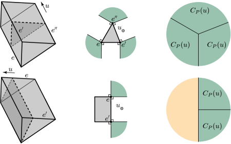
The notion of an aggregated cone at an edge direction is illustrated in Figures 2 and 1. Figure 1 shows a triangular prism and two of its aggregated cones. At the top of the figure, is the edge direction of parallel to the three edges , , and of that are not contained in a triangular face. The orthogonal projection of along is depicted at the center of the figure. In that case, coincides with as shown on the right of the figure. At the bottom of Figure 1, is an edge direction parallel to two edges and , each contained in one of the triangular faces of and is the half-plane depicted on the right of the figure. Again, the orthogonal projection of along is shown at the center of the figure. Note that has exactly three edge directions parallel to the edges of its triangular faces. In particular, up to symmetry, Figure 1 shows all the aggregated cones of a triangular prism.
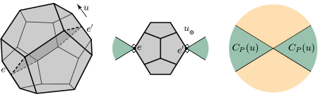
A regular dodecahedron and two of its opposite edges and are depicted on the left of Figure 2. Both of these edges are parallel to the same edge direction . The orthogonal projection of on is shown at the center of the figure and the aggregated cone is depicted on the right. It can be seen that is the union of two opposite cones that do not entirely cover . In particular, this illustrates that, while is always a cone, this cone is not always convex. It should be noted that is not equiprojective: its orthogonal projection on a plane parallel to a facet is a decagon while its orthogonal projection along a line through two opposite vertices is a dodecagon. However, an example of an equiprojective polytope with a non-convex aggregated cone—the equitruncated tetrahedron [10]—will be discussed in Section 6. Observe that, by the symmetries of the regular dodecahedron, the aggregated cones at the edges of this polytope are all equal up to isometry. In particular, Figure 2 depicts all the aggregated cones of the regular dodecahedron.
Note that a facet of has at most two edges parallel to any given edge direction of . Moreover, has exactly one edge parallel to if and only if the normal cone of at is one of the half-lines that compose the relative boundary of . We will use this in the proof of Theorem 1.3. This theorem is an equivalence and we shall prove two separate implications.
Lemma 3.6.
Consider a -dimensional polytope . If is equiprojective, then for any edge direction of , either
-
(i)
the aggregated cone is equal to or
-
(ii)
the relative interior of is equal to .
Proof.
Assume that is equiprojective and consider an edge direction of such that is not equal to . Let be a unit vector in the relative boundary of such that the relative interior of lies counter-clockwise from . Denote by the first unit vector in counter-clockwise from that is contained in the relative boundary of . Let us show in a first step that and both belong to the relative boundary of .
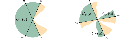
As discussed above, and span the normal cones of at two facets and , respectively, that each admit a unique edge parallel to . Denote these edges of and by and . Since is equiprojective, it follows from Theorem 3.2 that the edge-facet incidence must be compensated, but since doesn’t have another edge parallel to , there must exist a facet of distinct from but parallel to and an edge of parallel to such that the relative interiors of and are on the same side of the plane that contains these two edges. Now observe that cannot have another edge parallel to . Indeed the edge-facet incidence formed by such an edge with couldn’t be compensated by any other edge-facet incidence than but this one already compensates . Hence is in the relative boundary of . By symmetry, is also in the relative boundary of .
Since belongs to the relative boundary of , it cannot lie before counterclockwise from as shown on the left of Figure 3. Hence, , , and all the unit vectors between them counter-clockwise from are contained in a half-plane as shown on the right of the figure. As the relative interiors of and are on the same side of the plane that contains and , the relative interior of must lie clockwise from as shown on the right of Figure 3. Likewise, the relative interior of lies counter-clockwise from . In particular, all the unit vectors in counter-clockwise from and clockwise from must belong to . Indeed, otherwise one of these vectors would belong to the relative boundary of and, as we have just established, its opposite would be a unit vector in the relative boundary of that would lie before counter-clockwise from , contradicting our assumption on .
This shows that the relative interior of is contained in . By symmetry, one can exchange with the closure of in the above argument and the inverse inclusion therefore also holds. ∎
The following lemma states the other implication from Theorem 1.3. It will be proven via Theorem 3.2 by constructing an explicit partition of the set of all edge-facet incidences into compensating pairs.
Lemma 3.7.
If, for any edge direction of a -dimensional polytope ,
-
(i)
the aggregated cone is equal to or
-
(ii)
the relative interior of is equal to .
then is equiprojective.
Proof.
Assume that the condition in the statement of the lemma holds for any edge direction of a -dimensional polytope . We will partition the edge-facet incidences of into compensating pairs and the desired result will follow from Theorem 3.2. Consider a facet of and an edge of . Denote by the edge direction of parallel to and by the unit vector that spans the normal cone of at . We consider two mutually-exclusive cases.
First, assume that is the only edge of parallel to . In that case, is not equal to and belongs to the relative boundary of . According to assertion (ii), so does . Therefore, has a facet parallel to and distinct from that has a unique edge parallel to . By the same assertion, the relative interior of either lies counter-clockwise from and clockwise from or clockwise from and counter-clockwise from . As a consequence, the relative interiors of and lie on the same side of the plane that contains and . This shows that compensates and we assign these two edge-facet incidences to a pair in the announced partition. Observe that the same process starting with instead of would have resulted in the same pair of compensating edge-facet incidences of .
Now assume that has an edge parallel to other than . In that case, and compensate and we assign these two edge-facet incidences to a pair of the announced partition. Again, starting with instead of results in the same pair of edge-facet incidences of . Hence, repeating this process for all the edge-facet incidences of allows to form a partition of the edge-facet incidences of into compensating pairs, as desired. ∎
Theorem 1.3 is obtained by combining Lemmas 3.6 and 3.7. Let us illustrate this theorem on our examples from Figures 1 and 2. It is well known that a triangular prism is equiprojective [10, 11]. This can be immediately be recovered from Theorem 1.3 by observing that the aggregated cones of a triangular prism at its edge directions are either planes or half-planes as shown in Figure 1. In contrast, a regular dodecahedron is not equiprojective and this can also be obtained from Theorem 1.3. Indeed, the aggregated cones of a regular dodecahedron at its edge directions, depicted in Figure 2, are the union of two opposite cones that do not collectively cover the plane that they span.
4. Equiprojectivity and Minkowski sums
In this section, we exploit Theorem 1.3 in order to study the equiprojectivity of Minkowski sums. We will also determine the value of for which a polytope or a Minkowski sum of polytopes is -equiprojective.
Definition 4.1.
Consider an edge direction of a polytope contained in . The multiplicity of as an edge direction of is equal to when coincides with and to when it does not.
Note that, in Definition 4.1, can be a -dimensional polytope, a polygon or a line segment. From now on, we denote by the value of such that an equiprojective polytope is -equiprojective.
Theorem 4.2.
If is an equiprojective polytope, then
where the sum is over the edge directions of .
Proof.
Consider an equiprojective polytope contained in and a plane through the origin of that is not orthogonal to any of the facets of . Denote by the orthogonal projection on . Since is not orthogonal to any facet of , a line segment is an edge of if and only if it is the image by of an edge of such that the relative interior of intersects . Hence, is the number of the normal cones of at its edges whose relative interior is non-disjoint from . Let us count these normal cones of .
We consider an edge direction of and count the normal cones of at its edges parallel to , whose relative interior intersects . Since is not orthogonal to any facet of , the planes and are distinct and their intersection is a straight line . For the same reason, this line cannot contain any of the normal cones of at a facet. In other words, intersects exactly two normal cones of in their relative interior and these normal cones are at a vertex or at an edge of . According to Theorem 1.3, two cases are possible: either coincides with or the relative interior of is equal to . In the former case, is equal to and intersects the relative interior of two normal cones of at distinct edges parallel to . In the latter case, is equal to and intersects the relative interior of the normal cones of at an edge parallel to and at a vertex. Hence, summing over the edge directions of provides the desired equality. ∎
Now recall that the faces of the Minkowski sum of two polytopes and can be recovered from the normal cones of these polytopes (see for instance Proposition 7.12 in [22]): the faces of are precisely the Minkowski sums of a face of with a face of such that the relative interiors of and are non-disjoint. For this reason, Theorem 1.3 provides a convenient way to determine how equiprojectivity behaves under Minkowski sums.
Theorem 4.3.
Let and each be an equiprojective polytope, a polygon, or a line segment contained in . The Minkowski sum is equiprojective if and only if for each edge direction shared by and , either
-
(i)
or is equal to or
-
(ii)
coincides with or with .
Proof.
First assume that, for each edge direction of , at least one of the two assertions (i) and (ii) from the statement of the theorem holds. Pick an edge direction of such that is not equal to and let us prove that the relative interior of is equal to . It will then follow from Theorem 1.3 that is an equiprojective polytope.
Note that must be an edge direction of or one of . If is not an edge direction of both then it follows from (1) that the aggregated cone is equal to or to . In that case, Theorem 1.3 and Remark 3.5 imply that the relative interior of coincides with , as desired. If is an edge direction of both and , then by our assumption, either one of the cones and is equal to or the cone coincides with or with . However, is not equal to . Therefore, because of (1), this implies that coincides with . In that case, again by (1), is equal to and in turn, according to Theorem 1.3 and Remark 3.5, the relative interior of is equal to . It follows that is equal to , as desired.
Now assume that is equiprojective and that is an edge direction shared by and such that neither or is equal to . Observe that is a union of finitely many circular arcs and denote by the sum of the lengths of these arcs. Likewise, denote by and the sum of the lengths of the circular arcs contained in and in , respectively. Since and each are an equiprojective polytope, a polygon, or a line segment, whose aggregated cones at are not equal to , it follows from Theorem 1.3 and from Remark 3.5 that the relative interiors of and coincide with and , respectively. Hence, and are both equal to half the circumference of a unit circle. Also according to Theorem 1.3, either is equal to or the relative interior of coincides with . Therefore, is equal to the circumference of a unit circle or to half of it. In the former case, is equal to the sum of and . By (1), this can only happen when coincides with . In the latter case, , , and are equal and it follows from (1) that and coincide. ∎
Recall that the multiplicity of edge directions is defined for polygons and line segments and not just for -dimensional polytopes. From now on, if is a polygon or a line segment contained in , we denote
by analogy with Theorem 4.2, where the sum is over the edge directions of . It should be noted that when is a polygon, is equal to the number of edges of and when is a line segment, is always equal to .
Consider two polytopes and contained in . If each of them is an equiprojective polytope, a polygon, or a line segment, then we denote
where is the number of edge directions common to and such that both and are equal to while is the number of edge directions common to and such that the cones and are not both equal to and one of them is contained in the other.
Theorem 4.4.
Consider two polytopes and contained in , each of which is an equiprojective polytope, a polygon, or a line segment. If the Minkowski sum is an equiprojective polytope, then
Proof.
Assume that is equiprojective and consider an edge direction of . Note that is then an edge direction of or an edge direction of . It follows from Proposition 7.12 in [22] that
Hence, if is an edge direction of but not one of , then
| (2) |
and if is an edge direction of but not , then
| (3) |
If and share as an edge direction, we review the different possibilities given by Theorem 4.3 for how , and relate to one another. If both the aggregated cones and are equal to , then , and are all equal to . Hence,
| (4) |
If and are not both equal to , but one of these aggregated cones is contained in the other, then
Moreover, the smallest value between and is equal to . Hence,
| (5) |
Finally, if and are opposite and not equal to , then and are both equal to while is equal to . Therefore,
| (6) |
Observe that when two polytopes and do not share an edge direction, vanishes. Hence, we obtain the following corollary from Theorems 4.3 and 4.4. In turn, that corollary immediately implies Theorem 1.4.
Corollary 4.5.
Consider two polytopes and contained in , each of which is an equiprojective polytope, a polygon, or a line segment. If and do not share an edge direction, then is equiprojective and
5. Many -equiprojective polytopes when is odd
The goal of this section is to build many -equiprojective polytopes when is a large enough odd integer. This will be done using Minkowski sums between zonotopes with generators and well-chosen triangles. In this section, all the considered polytopes are contained in .
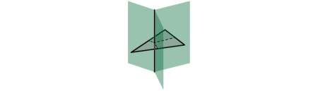
For any -dimensional zonotope , we consider a triangle whose edge directions do not belong to any of the planes spanned by two edge directions of and such that the plane spanned by the edge directions of does not contain any edge direction of . Note that such a triangle always exists because and have only finitely many edge directions. A consequence of these requirements is that does not share any edge direction with . Moreover, the normal cones of at its facets are never contained in the normal cone of at itself or in the plane spanned by the normal cone of at one of its edges (see Figure 4 for an illustration of the normal cones of a triangle at its edges and at itself). Inversely, the normal cone of at itself is not contained in the plane spanned by the normal cone of at any of its edges. It should be noted that there are many possible choices for but we fix that choice for each zonotope so that defines a map that sends a zonotope to a triangle.
It follows from the results of Section 4 that the Minkowski sum of with is always an equiprojective polytope.
Lemma 5.1.
If is a -dimensional zonotope with generators, then its Minkowski sum with is a -equiprojective polytope.
Proof.
Recall that the edge directions of are precisely the edge directions of and the edge directions of . By Proposition 2.1, is -equiprojective where is the number of generators of .
Now recall that when is a polygon, is equal to the number of edges of . As a consequence, is equal to and since does not share an edge direction with , it follows from Corollary 4.5 that the Minkowski sum of with is a -equiprojective polytope. ∎
Recall that the normal cones of a polytope ordered by reverse inclusion collectively form a lattice , called the normal fan of and that
is an isomorphism (see for instance Exercise 7.1 in [22]). Note that in this context, an isomorphism is a bijective morphism between two lattices. It will be important to keep in mind that reverses inclusion. This correspondence between the face lattice and the normal fan of a polytope will be useful in order to determine the combinatorial type of the Minkowski sum between a -dimensional zonotope and its associated triangle .
Further recall that a face of is uniquely written as the Minkowski sum of a face of with a face of . We will denote by the face of that appears in this Minkowski sum. Note that defines a morphism from the face lattice of to that of in the sense that it preserves face inclusion. This is a consequence, for instance of Proposition 7.12 from [22].
The remainder of the section is mostly devoted to proving that if and have the same combinatorial type, then so do and . This will be done via two lemmas. The first of these lemmas is the following.
Lemma 5.2.
Consider two -dimensional zonotopes and . If
is an isomorphism, then there is a commutative diagram
where is an isomorphism.
Proof.
Assume that is an isomorphism from the face lattice of to that of . Observe that has exactly two parallel triangular facets each of which is a translate of . Further observe that all the other facets of are centrally-symmetric, since they are the Minkowski sum of a centrally-symmetric polygon with a line segment or a point. The same observations hold for the Minkowski sum of with : that Minkowski sum has exactly two parallel triangular facets, each a translate of and its other facets all are centrally-symmetric. As induces an isomorphism between the face lattices of any facet of and the face lattice of , this shows that sends the two triangular facets of to the two triangular facets of . Moreover, two parallel edges of a centrally-symmetric facet of are sent by to two parallel edges of a centrally-symmetric facet of .
Recall that all the aggregated cones of are half-planes. As and do not have any edge direction in common, the aggregated cones of at the edge directions of are still half-planes. Note that the two half-lines that bound these half-planes are precisely the normal cones of at its triangular facets. Similarly, the aggregated cones of at the edge directions of are half-planes bounded by the normal cones of at its triangular facets. Since two parallel edges of a centrally-symmetric facet of are sent by to two parallel edges of a centrally-symmetric facet of , this implies that for every edge of , there exists an edge of such that any face of contained in is sent to by .
By the correspondence between face lattices and normal fans,
provides an isomorphism from to . Consider two edges and of and denote by the vertex they share. Let be the set of the normal cones of at its two triangular faces and at the faces contained in and in . Similarly, let denote the set made up of the normal cones of at its triangular faces and at the faces from and . By the above, is equal to . Moreover, it follows from Proposition 7.12 in [22] that and are polyhedral decompositions of the boundaries of the normal cone of at and of the normal cone of at the vertex shared by and . Observe that the boundaries of these normal cones (that are depicted in Figure 4) each separate into two connected components. As is an isomorphism from to , it must then send the normal cones of at the faces from to the normal cones of at the faces from . In other words, any face of contained in is sent to by . Hence, setting to results in the desired isomorphism . ∎
Recall that, for an arbitrary -dimensional zonotope , a face of is the Minkowski sum of a unique face of with . We will denote by the face of that appears in this sum. This defines a morphism from to . We will derive a statement similar to Lemma 5.2 regarding . In order to do that, we first establish the following proposition as a consequence of our requirements for the choice of .
Proposition 5.3.
Consider a -dimensional zonotope and two proper faces and of . If is a facet of , then either
-
(i)
coincides with or
-
(ii)
coincides with .
Proof.
Let us first assume that is a facet of and an edge of . It follows from our choice for that every polygonal face of is the Minkowski sum of a facet of with a vertex of , of a vertex of with itself, or of an edge of with an edge of . If is a polygon and a vertex of then it is immediate that is the Minkowski sum of an edge of with and therefore, coincides with . Similarly, if is a vertex of and is equal to , then must be an edge of and is equal to . Now if is an edge of and an edge of , then observe that is a parallelogram. As is an edge of , it must be a translate of either or . In the former case, is equal to and in the latter, is equal to , as desired.
Finally, assume that is an edge of and a vertex of . Recall that and do not share an edge direction. As a consequence, either is an edge of and a vertex of or inversely, is a vertex of and an edge of . In the former case, is equal to and in the latter coincides with , which completes the proof. ∎
We can now prove the following statement similar to that of Lemma 5.2.
Lemma 5.4.
Consider two -dimensional zonotopes and . If
is an isomorphism, then there is a commutative diagram
where is an isomorphism.
Proof.
Consider a proper face of and let us show that all the faces of contained in have the same image by . Assume for contradiction that this is not the case and recall that by Proposition 7.12 from [22], the normal cone is decomposed into a polyhedral complex by the normal cones of it contains. Since is convex and
is an isomorphism, must contain two faces and whose images by differ and such that the normal cone of at is a facet of the normal cone of at . By the correspondence between the face lattice of a polytope and its normal fan, is a facet of . Now recall that
and
It follows that must differ from as and would otherwise be equal. Hence, by Lemma 5.2, and have different images by . As they also have different images by and as is a facet of , this contradicts Proposition 5.3. As a consequence, all the faces of contained in have the same image by . In other words, there exists a face of such that sends to a subset of . In fact, this subset is necessarily itself. Indeed, observe that
is a partition of . Similarly,
is a partition of . As is a bijection, it must then send precisely to . It follows that is a bijection from to such that is equal to , as desired.
Finally, if is a face of and a face of , then observe that some face of from must be contained in a face from . Since is a morphism, this shows that is a face of . Hence is an isomorphism from the face lattice of to that of . ∎
The following is an immediate consequence of Lemma 5.4.
Lemma 5.5.
Consider two -dimensional zonotope and . If the Minkowski sums and have the same combinatorial type, then the zonotopes and have the same combinatorial type.
Consider an odd integer greater than or equal to (under this assumption, there exist zonotopes with generators). It follows from Lemmas 5.1 and 5.5 that the number of different combinatorial types of -equiprojective polytopes is at least the number of zonotopes with generators. Hence, Theorem 1.1 in the case of the -equiprojective polytopes such that is odd follows from Theorem 1.2 and from the observations that
and that
as goes to infinity.
6. Equiprojective polytopes and decomposability
Our results show that Minkowski sums allow for a sequential construction of equiprojective polytopes, thus providing a partial answer to Shephard’s original question. Two of the possible kinds of summands in these Minkowski sums, line segments and polygons, are well understood. However, equiprojective polytopes can also appear as a summand, and one may ask what the primitive building blocks of these sequential Minkowski sum constructions look like. More precisely, recall that a polytope is decomposable when it can be written as a Minkowski sum of two polytopes, none of which is homothetic to [12, 16, 18, 21]. This notion appears naturally within the study of the deformation cones of polytopes [14] and in particular in the case of the submodular cone [15]. It also appears in the study of the diameter of polytopes [4].
We ask the following question in the spirit of Shephard’s.
Question 6.1.
Are there indecomposable equiprojective polytopes?
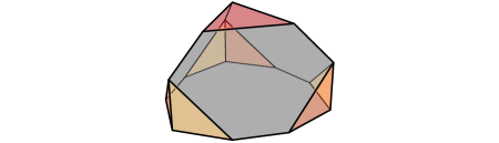
According to Lemma 3.7, any -dimensional polytope whose aggregated cones at all edge directions are planes or half-planes is necessarily equiprojective. These equiprojective polytopes form a natural superset of the zonotopes since the aggregated cones of -dimensional zonotopes at their edge directions are planes. It should be noted that this superset of the zonotopes does not contain all equiprojective polytopes. For instance, the equitruncated tetrahedron described in [10] has an aggregated cone at an edge direction that is neither a plane nor a half-plane. This equiprojective polytope is shown in Figure 5. It is obtained by cutting a tetrahedron along seven planes. The nonagonal face and the three hexagonal faces colored gray in the figure are what remains of the triangular faces of . The seven triangular faces of the equitruncated tetrahedron each result from one of the cuts. Six of these triangular faces are incident to the nonagonal face and colored yellow and orange in Figure 5. They all have a common edge direction orthogonal to the nonagon. Moreover, each of them shares a single edge direction with . The seventh triangular face, colored red in the figure, is parallel to the nonagonal face. It is not hard to see that the aggregated cone of the equitruncated tetrahedron at the edge direction orthogonal to the nonagonal face is the union of three cones whose pairwise intersection is reduced to the origin of . In particular, this aggregated cone is distinct from both a plane and a half-plane. This is another example of a non-convex aggregated cone. One can also see on the figure that the aggregated cones of the equitruncated tetrahedron at all of its other edge directions are half-planes. Note that this polytope is decomposable and in particular, it admits a tetrahedron homothetic to as a summand.
Finally, observe that, if the aggregated cone of a -dimensional polytope at some of its edge directions is a plane, then that polytope is decomposable (see for example [4]). However, the above question on polytope decomposability is open for the -dimensional polytopes whose aggregated cones at all edge directions are half-planes. By the above, these polytopes form a subclass of the equiprojective polytopes disjoint from zonotopes.
Question 6.2.
Does there exist an indecomposable -dimensional polytope whose aggregated cones at all edge directions are half-planes?
Acknowledgements. We are grateful to Xavier Goaoc for useful comments on an early version of this article and to anonymous referees for helpful suggestions and remarks. The PhD work of the first author has been partially funded by the MathSTIC (CNRS FR3734) research consortium.
References
- [1] Noga Alon, The number of polytopes, configurations and real matroids, Mathematika 33 (1986), no. 1, 62–71.
- [2] Anders Björner, Michel Las Vergnas, Bernd Sturmfels, Neil White, and Gunter M. Ziegler, Oriented matroids, Cambridge University Press, 1999.
- [3] Hallard T. Croft, Kenneth J. Falconer and Richard K. Guy, Unsolved problems in geometry, Springer New York, NY, 1991.
- [4] Antoine Deza and Lionel Pournin, Diameter, decomposability, and Minkowski sums of polytopes, Canadian Mathematical Bulletin 62 (2019), no. 4, 741–755.
- [5] David Eppstein, Forbidden configurations in discrete geometry, Cambridge University Press, 2018.
- [6] Stefan Felsner and Jacob E. Goodman, Pseudoline arrangements, Handbook of Discrete and Computational Geometry, third edition (Jacob E. Goodman, Joseph O’Rourke and Csaba D. Tóth, eds.), CRC Press, Boca Raton, FL, 2017, pp. 125–157.
- [7] Xavier Goaoc and Emo Welzl, Convex hulls of random order types, Journal of the ACM 70 (2020), no. 1, article no. 8.
- [8] Jacob E. Goodman and Richard Pollack, Multidimensional sorting, SIAM Journal on Computing 12 (1983), no. 3, 484–507.
- [9] Jacob E. Goodman and Richard Pollack, Upper bounds for configurations and polytopes in , Discrete & Computational Geometry 1 (1986), no. 3, 219–227.
- [10] Masud Hasan, Mohammad Monoar Hossain, Alejandro López-Ortiz, Sabrina Nusrat, Saad Altaful Quader, and Nabila Rahman, Some non-trivial examples of equiprojective polyhedra, Geombinatorics 31 (2022), no. 4, 170–177.
- [11] Masud Hasan and Anna Lubiw, Equiprojective polyhedra, Computational Geometry 40 (2008), no. 2, 148–155.
- [12] Michael Kallay, Indecomposable polytopes, Israel Journal of Mathematics 41 (1982), 235–243.
- [13] Jiří Matoušek, Order types and the same-type lemma, Lectures on Discrete Geometry, Graduate Texts in Mathematics, vol. 212, Springer, 2002, pp. 215–223.
- [14] Walter Meyer, Indecomposable polytopes, Transactions of the American Mathematical Society 190 (1974), 77–86.
- [15] Arnau Padrol, Vincent Pilaud and Germain Poullot, Deformed graphical zonotopes, Discrete & Computational Geometry, to appear (2021).
- [16] Krzysztof Przesławski and David Yost, Decomposability of polytopes, Discrete & Computational Geometry 39 (2008), 460–468.
- [17] Jürgen Richter-Gebert and Günter M. Ziegler, Oriented matroids, Handbook of Discrete and Computational Geometry, third edition (Jacob E. Goodman, Joseph O’Rourke and Csaba D. Tóth, eds.), CRC Press, Boca Raton, FL, 2017, pp. 159–184.
- [18] Geoffrey C. Shephard, Decomposable convex polyhedra, Mathematika 10 (1963), 89–95.
- [19] Geoffrey C. Shephard, Twenty problems on convex polyhedra part I, The Mathematical Gazette 52 (1968), no. 380, 136–147.
- [20] Geoffrey C. Shephard, Twenty problems on convex polyhedra part II, The Mathematical Gazette 52 (1968), no. 382, 359–367.
- [21] Zeev Smilansky, Decomposability of polytopes and polyhedra, Geometriae Dedicata 24 (1987), no. 1, 29–49.
- [22] Günter M. Ziegler, Lectures on polytopes, Graduate Texts in Mathematics, vol. 152, Springer, 1995.