Many-body multipole indices revealed by the real-space dynamical mean-field theory
Abstract
The multipole moments are fundamental properties of insulators, and have attracted lots of attention with emerging of the higher-order topological insulators. A couple of ways, including generalization of the formula for the polarization and the Wilson loop, have been proposed to calculate it in real materials. However, a practical method to explore it in correlated insulators is still lacking. Here, we proposed a systematic way, which combines the general Green’s function formula for multiopoles with the real-space dynamical mean-field theory, to calculate the multipole moments in correlated materials. Our demonstrating calculations are consistent with symmetry analysis, and the calculations of the spectral functions further confirm our results. This method opens the new avenue to study the topological phase transitions in correlated multipole insulators and other crucial physical quantities closely related to multipole moments.
I introduction
The polarization is a fundamental property of insulators, and it has been under intensive study for decades [1, 2, 3, 4, 5, 6, 7]. It is a ground-breaking progress to realize that the change of polarization is closely related to the integral of the Berry curvature in the parameter space [1, 2]. The emergence of topological insulators offers a new platform for the study of polarization, which works as a topological index for the topological phase transition. However, for a long time, a systematic method to reveal the polarization in a correlated insulator remains elusive, even if there are detailed discussion on this formalism [4, 8]. In Resta’s pioneering work [9], a formula for the polarization is proposed, and affords the possibility of exploring the polarization in the interacting case. Furthermore, with the concept of localization length [10], its connection with Kohn’s theory of insulating state [11] has been established. To explore the properties of multipole moments, which offers a distinctive point of view to uncover the nontrivial topological physics, is fundamentally important.
The topics on the polarization and its multipole generalization have become more active with the generalized concept of higher-order topological insulator. The higher-order topological phase, which is a key playground for multipole indices, is characterized by the quantized multipole indices, pioneered by Benalcazar et al. [12]. This novel concept has been identified in different non-crystalline lattices without periodicity [13, 14]. The generalization of Resta’s formula to the multipole case has opened the avenue to study the multipole [15], which can serve as an index to classify the higher-order topological insulators. Even though a couple of issues have been pointed out in this generalization [16], detailed calculations have been done for non-interacting models [17], and its effectiveness has been verified. Its relationship with the Wilson-loop formulation [12, 18] has been elaborated. Furthermore, several ways have been tried out to study multipole indices of correlated insulator. In Ref. [19], the polarization of the Hubbard model is explored with the dynamical mean-field theory (DMFT) [20]. However, it is hard to apply it to the multipole moments. In Ref. [21], correlation effects in quadrupole insulators are studied with the quantum Monte Carlo simulations and topological Hamiltonians. In Ref. [22] a many-body invariant is extracted from Resta’s operator for the polarization with methods of exact diagonalization and infinite density matrix renormalization group. Clearly, these are indirect ways to calculate the multipole indices in correlated systems.
However, a practical procedure for directly calculating the many-body multipole index of correlated insulators is still lacking. Here, we propose a Green’s function formalism in the real space for the multipole indices, which can be perfectly fitted into the scheme of the real-space dynamical mean-field theory (R-DMFT) [23, 24, 25]. We have carried out calculations of multipole indices of the correlated Benalcazar-Bernevig-Hughes (BBH) model with different spatial symmetries. The results are consistent with the symmetry analysis, and shed light on the exploration of multipole indices of the correlated insulator. Furthermore, we would like to point out that our formalism can be adopted to study the higher-order topological phase in crystalline systems with quenched disorder and in non-crystalline systems, and that it also affords a way to compute the localization length of the electron [10], the polarization fluctuation [26], and the quantum geometric tensor [27] in the correlated lattices.
The rest of the manuscript has been organized as follows. In Sec. II, we show our derivation details for the general formula of the multipoles, explain our protocol on how to combine them with the R-DMFT, and point out its further generalization. In Sec. III, we show our demonstrating calculation results for the correlated BBH model with different spatial symmetries. A summary and outlook is presented in Sec. IV.
II Many-body multipole indices in Green’s function formalism
We propose a Green’s function formalism for the electrical polarization for a crystal, which is ready to be studied in a correlated system,
| (1) |
This is the central result in this work. Here . , and is a matrix of Green’s function with the -th element as , where is the Matsubara frequency, and () is the creation (annihilation) operator on the lattice site () in a supercell with sizes as , , and for one, two and three-dimensional cases, respectively. is the identity matrix. is dimension-dependent as , , for different dimensions, which is the area perpendicular to the direction. is the contribution from the background charge, with the local density of electrical states. It can be combined with fixed boundary condition, periodic boundary condition and a hybrid boundary condition. The generalization to include the spin flavor is straightforward.
We outline the crucial derivation steps for Eq. (1). Starting from the formula [9, 15], , where , we have,
| (2) |
For the electron, we note the nilpotency property of the electron number operator , which is a key observation here, and it follows that with . Therefore, we come to
| (3) | ||||
| (4) |
where the last step is obtained by a direct multiplication. We define a matrix , with , (). A second key observation [28] is that different orders of principal minors for coincides with different order of terms for in Eq. (4) with Wick’s theorem. As an example, we can see that the second order of principal minors of are , with , which coincide with in Eq. (4) by using Wick’s theorem to the latter form. Furthermore, assuming eigenvalues for are (), we have an identity for with eigenvalues as [29],
| (5) |
Compared with the characteristic polynomials , and setting , we find
| (6) |
Therefore, finally we have the polarization in the formalism of Green’s functions,
| (7) |
With the identity , we have obtained Eq. (1). We have a remark here for the numerical implementation. As is known that polarization is an intensive quantity. In practical calculations, one cannot adopt Eq. (7), of which the first term tends to go to zero in the thermodynamic limit in the more than one-dimensional space [30], because numerically the imaginary part of the logarithm function lies in the interval .
Similarly, we can write down the formula for the quadrupole moment in a crystal,
| (8) |
Here , and . , for two- and three-dimensional case, which is the length perpendicular to the plane. . A generalization to the case of the octupole moment is straightforward.
The key issue in the calculations in Eqs. (1) and (8) is to obtain the matrix of Green’s function , and we are interested in correlated systems described by the fermionic Hubbard model. It is necessary to obtain of a correlated lattice model for calculating of many-body multipole moments. Real-space dynamical mean-field theory (R-DMFT) [20, 23, 24, 25] is perfectly suitable for this purpose. In this scheme, a strongly correlated system on a lattice is mapped into a group of impurities on lattice sites with the same spatial symmetry, along with hopping between different sites. In this way both the onsite interactions and the inhomogeneous due to hopping are taken into account. One then solves the DMFT problem on all the sites until it is fully converged. Therefore, the interaction effects are taken into account on the DMFT level. Once the R-DMFT loop is converged, we then adopt Eqs. (1) and (8) to compute multipole indices. The flow chart for the whole computation process is shown in Fig. 1, which can be mostly divided into two parts: (1) the R-DMFT part, and (2) the computation of many-body multipole indices. We comment on the efficiency of this algorithm. The most time-consuming part would be the R-DMFT routines, which can be accelerated with parallel implementation and optimized by the spatial symmetry consideration. With convergent Green’s function, the calculations of multipole indices are quite efficient.
To sum up, we have achieved two significant advancements. (1) We have a formula in the formalism of real-space Green’s functions for the multipole indices, which is ready to be combined with the DMFT method, and one can further introduce disorders to lattices to explore the rich physics of disorder effects, quasi-crystal lattice [31], amorphous lattices [32, 33] and so on. (2) With the multipole indices as a bridge, one can certainly study the localization length of the electron [10], the polarization fluctuation [26], and the quantum geometric tensor [27] in the correlated lattices.

III Demonstrating R-DMFT calculations of the interacting BBH model with staggered potentials
In this section, we implement the multipole moment of the correlated BBH model based on Eqs. (1) and (8) with the real-space Green’s function calculated by the R-DMFT, and discuss the correlation effects explicitly.
III.1 The interacting BBH Model
The interacting BBH model [12, 18] on a two-dimensional lattice with the Hubbard interaction and staggered potentials reads,
where
and is the onsite staggered potential. The non-interacting part is a standard toy model of the higher-order topological insulator. In general, spatial symmetries are closely related the quantization of the polarization and quadrupole moments [12, 18]. By the term we can tune the spatial symmetry, and explore the correlating effects by introducing the Hubbard interaction term. We are mainly interested into two cases with different spatial symmetries as follows: case (i) preserving the spatial inversion symmetry, and case (ii) or which respects mirror symmetry along the -direction (or the -direction).
III.2 Results and discussion
As a demonstration for our general protocol to calculate the multipole indices in correlated insulators, we present results for the polarization and quadrupole moments of the interacting BBH model when the onsite staggered potential is nonzero, which affords us a way to tune the spatial symmetry. For the R-DMFT part calculations, an impurity solver of iterative perturbation theory [20] is adopted. We choose the periodical boundary conditions for lattices, work at the half-filling with , and focus on the paramagnetic phase. As a side remark, we point out that all the multipole moments data are presented by modulo 1.
III.2.1 Case (i)
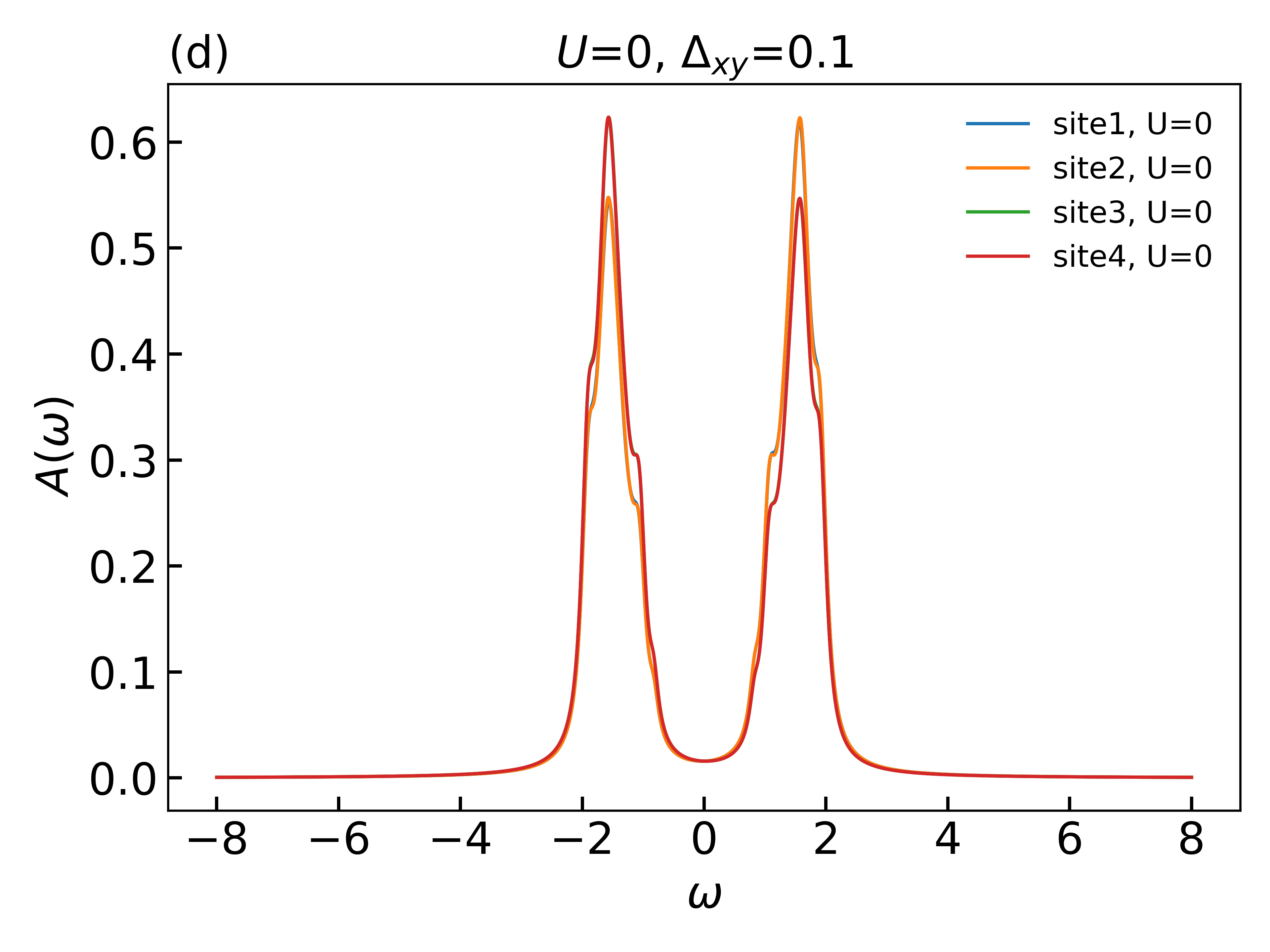
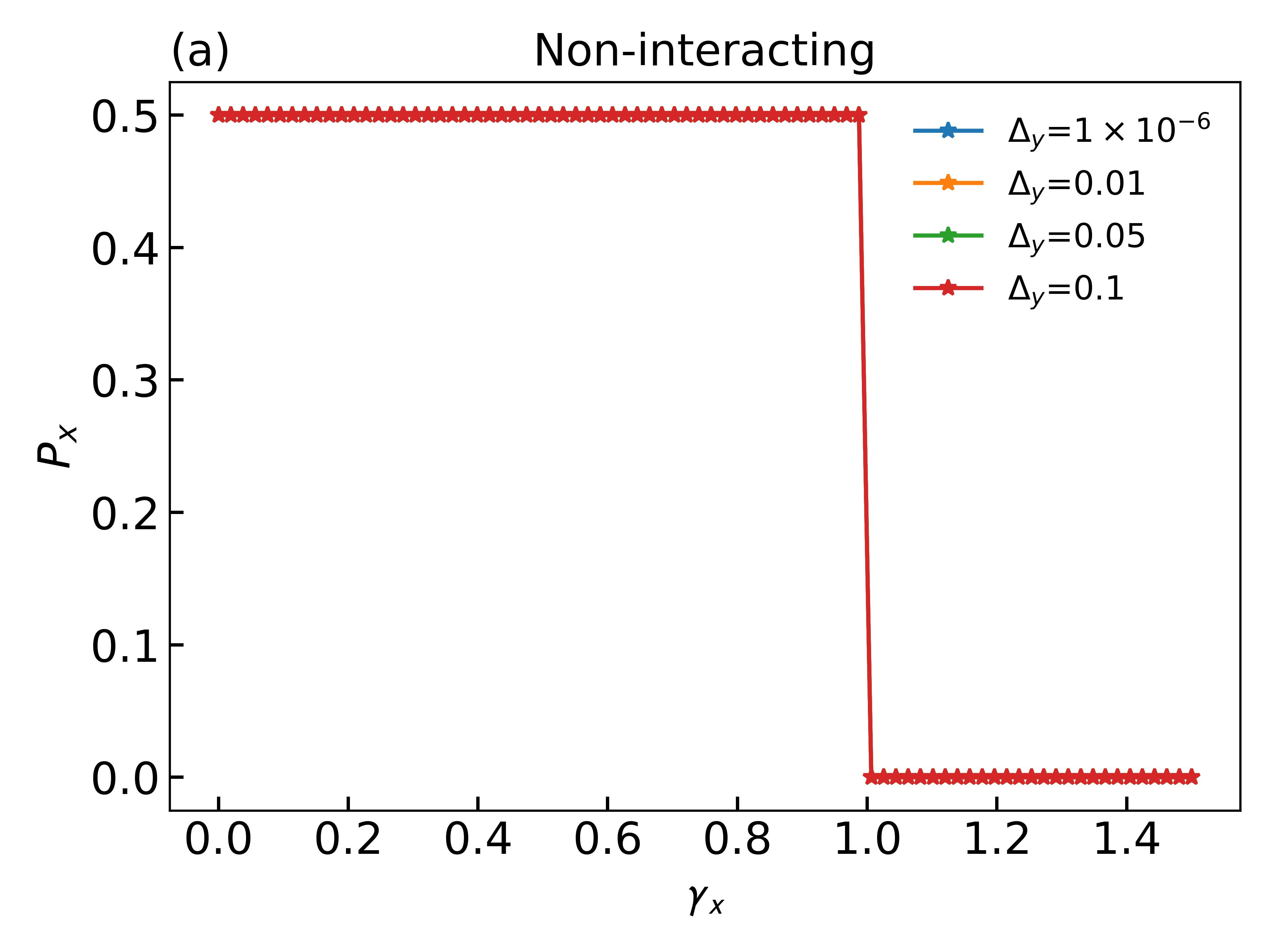
As shown in Fig. 2, there are quantized polarization component and sharp topological phase transitions in non-interacting case, which are features of the BBH model, and remarkably similar phenomena in interacting regimes. The results given by the formula (1) are consistent with the spatial symmetry analysis. In Fig. 2, we do not present results for , whose features are quite similar to these for . The onsite staggered potential breaks the reflection symmetries about both and axes, but keeps the inversion symmetry, which leaves the polarization quantized in Fig. 2 for non-interacting case (a), weakly interacting case (b) and strongly interacting case (c). Within the R-DMFT method, even though the interaction is turned on, the polarization component keep quantized as long as the spatial symmetry conditions for quantization are preserved. In Fig. 2, we show the spectral functions for four different sites in one unit cell, and the gaps due to interactions together with emergent side-bands in Figs. 2(e-f) for very strong interactions clearly show that the system is driven into the Mott insulator phase when the interaction is large enough. To sum up, we show that even in the correlating regime, the quantization of polarization is still determined by the spatial symmetries.
Furthermore, we present our results for the quadrupole moment calculations with Eq. (8) in Fig. 3. If the reflection symmetries are absent, the quadrupole moment is unquantized in Figs. 3(a) with nonzero , and (c) with both and interaction turned on. As long as the reflection symmetry is preserved in both and directions, the quadrupole moment stays quantized as shown in Fig. 3(b). It shows that the spatial symmetry is a dominant factor for the quantization of the quadrupole moment in the paramagnetic phase.


III.2.2 Case (ii)
In this subsection, we present our results for the polarization and for case (ii) with , which respects the mirror symmetry in the direction. In Fig. 4(a) for non-interacting case with different strengths of , (b) for weak interactions with finite and (c) for strong interaction with finite , we observe perfect quantization of the polarization and clear topological transition when both the interaction and is finite. Due to the spatial symmetry of case (ii), the topological transition here is in fact quite similar to that in the one-dimensional Su-Schrieffer-Heeger model [35]. As a sharp contrast in Figs. 4(d-f), we can see the quantization of is broken once is nonzero, indicating the broken of the mirror symmetry. By the comparison between and , we clearly see that the spatial symmetry is a vital factor for the quantization of the polarization in the paramagnetic phase. As a side comment, in Figs. 4(a, d), we introduce a tiny to break the mirror symmetry with the axis a little, as a numerical trick to remove the “degeneracy” between and for the polarization in the sense of modulo [18].


IV Summary and outlook
To sum up, we propose a practical calculation scheme for the multipole moments in correlated materials on the level of R-DMFT. By calculations of BBH with different spatial symmetries due to staggered potentials, and different strengths of interactions we show the effectiveness of our method in exploring the properties of the multipole indices. However, its full potential is not fully unleashed. Our general method is ready to be implemented to explore a disordered correlated lattice. The close relation of polarization with the localization length [10], and the quantum geometric tensor [27] affords us a way to explore these interesting physical quantities. Our demonstrating calculations show that the spatial symmetry is a dominant factor for the quantization of the polarization and quadrupole moments even in the correlating regime, at least in the paramagnetic phase.
Acknowledgements.
T.Q. and J.H.Z. were supported by the National Natural Science Foundation of China under Grants No.12174394 and U2032164. J.H.Z. was also supported by HFIPS Director’s Fund (Grants No. YZJJQY202304 and No. BJPY2023B05) and Anhui Provincial Major S&T Project (s202305a12020005), the High Magnetic Field Laboratory of Anhui Province under Contract No. AHHM-FX-2020-02. A portion of this work was supported by Chinese Academy of Sciences under contract No. JZHKYPT-2021-08.References
- Resta [1992] R. Resta, Ferroelectrics 136, 51 (1992).
- King-Smith and Vanderbilt [1993] R. D. King-Smith and D. Vanderbilt, Phys. Rev. B 47, 1651 (1993).
- Resta [1994] R. Resta, Rev. Mod. Phys. 66, 899 (1994).
- Ortiz and Martin [1994] G. Ortiz and R. M. Martin, Phys. Rev. B 49, 14202 (1994).
- Coh and Vanderbilt [2009] S. Coh and D. Vanderbilt, Phys. Rev. Lett. 102, 107603 (2009).
- Xiao et al. [2010] D. Xiao, M.-C. Chang, and Q. Niu, Rev. Mod. Phys. 82, 1959 (2010).
- Vaidya et al. [2024] S. Vaidya, M. C. Rechtsman, and W. A. Benalcazar, Phys. Rev. Lett. 132, 116602 (2024).
- Ortiz et al. [1996] G. Ortiz, P. Ordejón, R. M. Martin, and G. Chiappe, Phys. Rev. B 54, 13515 (1996).
- Resta [1998] R. Resta, Phys. Rev. Lett. 80, 1800 (1998).
- Resta and Sorella [1999] R. Resta and S. Sorella, Phys. Rev. Lett. 82, 370 (1999).
- Kohn [1964] W. Kohn, Phys. Rev. 133, A171 (1964).
- Benalcazar et al. [2017a] W. A. Benalcazar, B. A. Bernevig, and T. L. Hughes, Science 357, 61 (2017a).
- Xie et al. [2021] B. Xie, H.-X. Wang, X. Zhang, P. Zhan, J.-H. Jiang, M. Lu, and Y. Chen, Nat Rev Phys 3, 520 (2021).
- Yang et al. [2024] Y.-B. Yang, J.-H. Wang, K. Li, and Y. Xu, J. Phys.: Condens. Matter 36, 283002 (2024).
- Kang et al. [2019] B. Kang, K. Shiozaki, and G. Y. Cho, Phys. Rev. B 100, 245134 (2019).
- Ono et al. [2019] S. Ono, L. Trifunovic, and H. Watanabe, Phys. Rev. B 100, 245133 (2019).
- Lee et al. [2022] W. Lee, G. Y. Cho, and B. Kang, Phys. Rev. B 105, 155143 (2022).
- Benalcazar et al. [2017b] W. A. Benalcazar, B. A. Bernevig, and T. L. Hughes, Phys. Rev. B 96, 245115 (2017b).
- Nourafkan and Kotliar [2013] R. Nourafkan and G. Kotliar, Phys. Rev. B 88, 155121 (2013).
- Georges et al. [1996] A. Georges, G. Kotliar, W. Krauth, and M. J. Rozenberg, Rev. Mod. Phys. 68, 13 (1996).
- Peng et al. [2020] C. Peng, R.-Q. He, and Z.-Y. Lu, Phys. Rev. B 102, 045110 (2020), publisher: American Physical Society.
- Kang et al. [2021] B. Kang, W. Lee, and G. Y. Cho, Phys. Rev. Lett. 126, 016402 (2021).
- Potthoff [2003] M. Potthoff, Eur. Phys. J. B 32, 429 (2003).
- Helmes [2008] R. Helmes, Dynamical Mean Field Thoery of inhomogeneous correlated systems, PhD Thesis, Koln University (2008).
- Hofstetter and Qin [2018] W. Hofstetter and T. Qin, Journal of Physics B: Atomic, Molecular and Optical Physics 51, 082001 (2018).
- Resta [2006] R. Resta, Phys. Rev. Lett. 96, 137601 (2006).
- Souza et al. [2000] I. Souza, T. Wilkens, and R. M. Martin, Phys. Rev. B 62, 1666 (2000).
- Cheong and Henley [2004] S.-A. Cheong and C. L. Henley, Phys. Rev. B 69, 075111 (2004).
- Meyer [2023] C. D. Meyer, Matrix Analysis and Applied Linear Algebra, Second Edition (Society for Industrial and Applied Mathematics, Philadelphia, PA, 2023).
- Resta [2021] R. Resta, J. Chem. Phys. 154, 050901 (2021).
- Tran et al. [2015] D.-T. Tran, A. Dauphin, N. Goldman, and P. Gaspard, Phys. Rev. B 91, 085125 (2015).
- Agarwala and Shenoy [2017] A. Agarwala and V. B. Shenoy, Phys. Rev. Lett. 118, 236402 (2017), publisher: American Physical Society.
- Yang et al. [2019] Y.-B. Yang, T. Qin, D.-L. Deng, L.-M. Duan, and Y. Xu, Phys. Rev. Lett. 123, 076401 (2019).
- Vidberg and Serene [1977] H. J. Vidberg and J. W. Serene, Journal of Low Temperature Physics 29, 179 (1977).
- Su et al. [1980] W. P. Su, J. R. Schrieffer, and A. J. Heeger, Phys. Rev. B 22, 2099 (1980).
- Yatsugi et al. [2022] K. Yatsugi, T. Yoshida, T. Mizoguchi, Y. Kuno, H. Iizuka, Y. Tadokoro, and Y. Hatsugai, Commun Phys 5, 180 (2022).
- Dong et al. [2021] J. Dong, V. Juričić, and B. Roy, Phys. Rev. Res. 3, 023056 (2021), publisher: American Physical Society.