Many-body localization in one dimensional optical lattice with speckle disorder
Abstract
The many-body localization transition for Heisenberg spin chain with a speckle disorder is studied. Such a model is equivalent to a system of spinless fermions in an optical lattice with an additional speckle field. Our numerical results show that the many-body localization transition in speckle disorder falls within the same universality class as the transition in an uncorrelated random disorder, in contrast to the quasiperiodic potential typically studied in experiments. This hints at possibilities of experimental studies of the role of rare Griffiths regions and of the interplay of ergodic and localized grains at the many-body localization transition. Moreover, the speckle potential allows one to study the role of correlations in disorder on the transition. We study both spectral and dynamical properties of the system focusing on observables that are sensitive to the disorder type and its correlations. In particular, distributions of local imbalance at long times provide an experimentally available tool that reveals the presence of small ergodic grains even deep in the many-body localized phase in a correlated speckle disorder.
I Introduction
Isolated quantum many-body systems are generically expected to reach thermal equilibrium according to eigenstate thermalization hypothesis Deutsch (1991); Srednicki (1994); Rigol et al. (2008); D’Alessio et al. (2016). The approach to thermal equilibrium may be precluded by strong disorder resulting in phenomenon of Many-Body Localization (MBL) Gornyi et al. (2005); Basko et al. (2006) investigated in recent years both theoretically and experimentally (for reviews see Huse et al. (2014); Nandkishore and Huse (2015); Alet and Laflorencie (2018); Abanin et al. (2019)). Further examples of nonergodic many body-systems include models with constrains Sala et al. (2020); Khemani et al. (2020); Rakovszky et al. (2020), lattice gauge theories Smith et al. (2017); Brenes et al. (2018); Magnifico et al. (2020); Chanda et al. (2020a); Giudici et al. (2020); Surace et al. (2020) often linked with periodic oscillatory behavior coined, in the wake of well known quantum chaos notion Heller (1984); Bogomolny (1988), as quantum scarring Turner et al. (2018); Ho et al. (2019); Khemani et al. (2019); Iadecola and Žnidarič (2019); Schecter and Iadecola (2019), as well as surprizingly basic systems as interacting particles in tilted lattices (Stark-like localization) Schulz et al. (2019); van Nieuwenburg et al. (2019) or even harmonic potentials featuring coexistence of localized and delocalized phases James et al. (2019); Chanda et al. (2020b); Yao and Zakrzewski (2020a).
The theoretical studies of MBL typically consider uniform uncorrelated random potential as a source of disorder in the system. In contrast, the experimental setups used much easier to realize quasiperiodic potential Schreiber et al. (2015); Choi et al. (2016) correlated at arbitrary length scales. The behavior of one-dimensional (1D) models deep in the localized phase is similar in both cases (leading e.g. to preservation of the information about initial states in time dynamics Schreiber et al. (2015); Choi et al. (2016)). The situation is more complicated in the crossover between localized and extended phases. It is claimed even that the observed behavior suggest different universality classes of MBL transition depending on the disorder type Khemani et al. (2017); Sierant and Zakrzewski (2019). For uncorrelated disorder one expects to observe the influence of rare events, the so called Griffiths regions Griffiths (1969); Vojta (2010) i.e. grains of the minority phase on the either side of the transition (e.g. presence of ergodic grains on the localized side). Those affect the time dynamics and lead to e.g. subdiffusive transport on the delocalized side Agarwal et al. (2015); Luitz et al. (2015); Agarwal et al. (2017); Gopalakrishnan et al. (2016); Luitz et al. (2016); Luitz and Lev (2017). Even though the rare Griffiths regions are a priori absent in the deterministic quasiperiodic potential, the resulting dynamics are similar as in the uncorrelated disorder featuring a power-law decay of time-correlators as well as a power-law growth of the entanglement entropy Luitz et al. (2016); Lüschen et al. (2017) - for a recent review see Gopalakrishnan and Parameswaran (2020).
Surpizingly much less is known about MBL in a random speckle potential, despite the fact that such a potential has been successfully used in single particle physics e.g. for the experimental demonstration of Anderson localization in cold atomic gases Billy et al. (2008); Piraud and Sanchez-Palencia (2013). For attractively interacting bosons the bright soliton can be trapped in a speckle-disorder potential and get Anderson localized Sacha et al. (2009); Delande et al. (2013). A study of MBL in two-dimensional continuum Nandkishore (2014) concludes that perturbation theory diverges for arbitrarily weak interactions in a speckle potential. Moreover, it is not clear whether the insulating state of a strongly correlated atomic Hubbard gas in a speckle potential observed in center-of-mass velocity measurements Kondov et al. (2015) can be attributed to MBL since the phenomenon is believed to be not stable beyond one dimension De Roeck and Huveneers (2017). A recent theoretical study of MBL in a speckle potential Mujal et al. (2019) was limited to few particles only due to numerical requirements of the continuum approach.

The aim of this work is to provide an in depth study of MBL in a speckle potential in a one dimensional chain which is the typical geometry in which MBL is studied both experimentally and theoretically. While MBL has been studied for spinless or spin-1/2 fermions Mondaini and Rigol (2015) as well as for bosons in optical lattices potential Sierant et al. (2017); Sierant and Zakrzewski (2018); Orell et al. (2019); Hopjan and Heidrich-Meisner (2020); Yao and Zakrzewski (2020b) we choose to consider the simplest, paradigmatic model used in MBL studies, namely, the disordered Heisenberg chain. There are at least two reasons underlying this choice. Firstly, for random uniform as well as quasiperiodic disorder the Heisenberg spin chain has been quite deeply analyzed already, thus a direct comparison with random uniform results allow us to better comprehend the differences resulting from the nature of the speckle potential. Secondly, with the local on-site Hilbert space dimension equal to 2, one may, using exact diagonalization approach reach system size of the order of straightforwardly. That allows us for an in-depth analysis of properties of the system. That would be much harder for bosons or spinful fermions – for the latter, in addition, the inherent SU(2) symmetry affects deeply the MBL transition Prelovšek et al. (2016); Zakrzewski and Delande (2018); Kozarzewski et al. (2018); Protopopov and Abanin (2019); Suthar et al. (2020).
The paper is organized as follows. Section II introduces the model and the speckle disorder, we review its basic properties there. With this knowledge we consider properties of eigevalues and eigenstates of the model in Section III while the time dynamics is discussed in Section IV. Appendices provide additional discussion on specialized topics. We summarize our findings in Section V.
II The model.
We consider a 1D Heisenberg spin chain, widely used in MBL studies Luitz et al. (2015); Agarwal et al. (2015); Bera et al. (2015, 2017); Herviou et al. (2019); Colmenarez et al. (2019). This model maps, via Jordan-Wigner transformation, to a system of interacting spinless fermions which allows us to make the connection with optical lattice experiments. Instead of quasiperiodic disorder imposed by a secondary weak optical lattice with period incommensurate with the primary lattice (in which the tight binding approximation is inherently assumed) as in experiments Schreiber et al. (2015); Lüschen et al. (2017) we imagine that the disorder is added by an additional optical potential due to a speckle radiation. This additional light may operate on a different optical transition than the primary optical lattice and, within the tight binding approximation for the latter, leads to a desired speckle disorder. The resulting Hamiltonian of the system reads:
| (1) |
where are spin-1/2 matrices, will be considered as the energy unit, open boundary conditions are assumed. The local magnetic fields, , are drawn from the speckle distribution where (an overbar denotes an average over disorder realizations). Similarly, is the standard deviation of the exponential distribution. Importantly, values may be correlated depending on their relative position. The speckle is typically generated by transmission of light through a ground glass plate Goodman (2007). The correlations in the speckle pattern result from interference of light scattered by different parts of the plate and are, therefore, controlled by the aperture of the object. Assuming a rectangular plate, see Lugan et al. (2009) for more details, the correlation function takes a form (in discrete representation) with and the distance (unit lattice constant assumed) - compare Fig. 1.
Few remarks are in order. The disorder is asymmetric with assumed positive . We could also change the sign of all to have an opposite case (in atomic implementation a change of the sign corresponds to the change of the sign of the detuning on the atomic transition). This sign is relevant and important for low lying states Sacha et al. (2009); Delande et al. (2013) (as the disorder corresponds to either peaks or valleys of the potential). However we shall consider highly excited states from the middle of the spectrum and this sign becomes irrelevant. Second, in an optical implementation may be as low as Billy et al. (2008) i.e. a fraction of the typical lattice spacing in experiment Schreiber et al. (2015); Lüschen et al. (2017). In the tight binding model we have then simply an uncorrelated disorder. Increasing we may study how finite correlations in the potential affect MBL, the option apparently not available for other types of experimentally relevant disorder used till now.
For reference, we shall use also the uniform random (UR) disorder, for which the fields are independent random variables drawn from uniform distribution on interval .
III Properties of eigenvalues and eigenstates
III.1 Locating the transition
With the model defined we study first its spectral properties to verify the presence of the ergodic-MBL transition. Consider a mean gap ratio, , calculated as an average of
| (2) |
where (with being eigenvalues of the system) and the average is taken over a region of spectrum and over disorder realizations. The mean gap ratio was proposed as a simple probe of level statistics in Oganesyan and Huse (2007) with for Poisson statistics (PS) (corresponding to localized, integrable case) and for Gaussian orthogonal ensemble (GOE) Mehta (1990); Haake (2010) of random matrices well describing statistically an ergodic system.

We determine the mean gap ratio as a function of the disorder amplitude for several system sizes. Since the total spin projection on the axis is conserved, we consider the largest nontrivial sector of the Hamiltonian with – that restricts system sizes considered to even. Typically, we consider about eigenenergies from the middle of the spectrum, i.e. where with being the lowest (highest) eigenvalue for a given disorder realization. The results are averaged over 1000 disorder realizations or twice that number close to the estimated transition point. Data for and are obtained by full exact diagonalization, the ones for and are obtained using POLFED algorithm Sierant et al. (2020a). The results are shown in Fig. 2. Curves corresponding to different system sizes cross typically in the vicinity of - this crossing point is taken as an estimate of the critical disorder value, for different disorders. We refrain from using the procedure of a single parameter finite size scaling Luitz et al. (2015); Mondaini and Rigol (2015); Khemani et al. (2017) as it has became apparent recently Laflorencie et al. (2020); Šuntajs et al. (2020) that the transition may be of Kosterlitz-Thouless type and such a finite size scaling approach may be not valid.
The critical values of disorder for for all considered models are given in Table I. Note that for UR disorder we get close to obtained with finite size scaling in the system with open boundary conditions Chanda et al. (2020c). The critical disorder values are used to rescale the disorder amplitude to facilitate a comparison between various models of disorder. From now on we shall use, whenever possible, the rescaled disorder, .
| UR | ||||
|---|---|---|---|---|
| 3.4 | 2.25 | 4 | 6.5 |
Comparison of Fig. 2(a) and Fig. 2(b) shows that the crossover between ergodic and localized phases for UR disorder is sharper than for the uncorrelated speckle disorder (). The disorder strength at which the average gap ratio departs from the GOE value reaches for the UR disorder and system size and for speckle disorder with . This can be traced back to the unbounded on-site distribution of the speckle potential: the probability of having a fully ergodic system at e.g. is diminished, in comparison to the UR disorder case, by the rare events in which the field is large on one of the sites. The effect of broadening of the crossover is further enhanced when the correlations () are introduced in the speckle potential.
This suggests that finite size effects are stronger for the correlated disorder which is seemingly contradicted by the fact that curves for different sizes are much closer to each other for the correlated speckle disorder. However, a weaker size dependence of is a sign of strong finite size effects – relatively small changes in system sizes available to exact diagonalization are simply too small to have a visible effect on dependence for the correlated speckle disorder.
III.2 Inter-sample randomness

A more detailed characteristic of ergodic to MBL transition is obtained when one examines variation of system properties for individual disorder realizations Sierant and Zakrzewski (2019). To that end we average the gap ratios obtained from eigenvalues from the middle of the spectrum () for a single disorder realization which yields a sample-averaged gap ratio . The distributions of (obtained from calculating for many disorder realizations) vastly differ between UR disorder and quasiperiodic potential Sierant and Zakrzewski (2019) pointing out the dominant role of inter-sample randomness in the MBL transition in the UR disorder. The large inter-sample randomness, in turn, may be linked to the existence of rare Griffiths regions. Hence, it was suggested Khemani et al. (2017) that MBL transitions for UR disorder and quasiperiodic potential belong to different universality classes.
The distribution of the sample averaged gap ratio obtained for the speckle disorder are compared with the UR disorder case in Fig. 3. Three values of the rescaled disorder are considered: and corresponding to delocalized and localized phases, respectively, and intermediate one corresponding to (for RU disorder ). Such intermediate values of disorder correspond to the maximal inter-sample randomness in the system with the biggest variance of the distribution and in the thermodynamic limit they tend to the respective critical values provided that MBL persists in the thermodynamic limit (this issue is a topic of the current debate Šuntajs et al. (2019); Panda et al. (2020); Sierant et al. (2020b, a); Šuntajs et al. (2020)).
Observe that, as it could be expected, the distributions for the localized and delocalized cases are quite similar for UR and for the speckle disorders with different correlation lengths. The situation is markedly different in the transition regime. For the system with UR disorder the distribution is unimodal, although broad. On the other hand, for the speckle disorder one can observe a bimodal shape. With the increase of the correlation length the two peaks observed for speckle potential become more pronounced and overlap more the distributions for delocalized and localized phases.
Apparently, the sample averaged gap ratio distribution catches an important difference between the speckle and UR disorder. The speckle distribution is exponential favoring small values of disorder. Thus, it is quite probable to obtain nearby sites with very small difference in the local potential – that facilitates transport. This observation may be quantified by finding the probability distribution for the difference between consecutive random numbers which, for speckle disorder is also exponential. At the intermediate rescaled disorder, , the probability of having an ergodic system is enhanced for the uncorrelated speckle disorder. At the same time, the unbounded exponential distribution may give rise to few sites with a significantly larger values of resulting in a localized sample , explaining the bimodal structure of the distribution for the speckle disorder with . This mechanism is further reinforced by the presence of correlations in the speckle potential ().
All in all, our results confirm that the inter-sample randomness plays a significant role in the ergodic-MBL transition both for the UR and speckle disorder. This suggests that both UR and speckle disorder correspond to the same universality class of MBL transition, dominated by strong fluctuations in sample-to-sample properties and interplay of ergodic and localized grains. This is in sharp contrast to the MBL transition in quasiperiodic potential observable in current experimental setups where the system properties are much more uniform Agrawal et al. (2020).
III.3 Participation entropies of eigenstates and multifractality
While gap ratio statistics provides statistical information about eigenvalues of the model, additional information may be gained from eigenvector properties. Those may be probed via e.g. participation entropies. Following Macé et al. (2019) we consider participation entropies defined via the -th moments of wavefunction following the exprespages = 036206,sion:
| (3) |
where are the coefficients of wavefunction in the basis state , i.e. , is the dimension of Hilbert space. While providing supplementary information to that hidden in eigenvalues one should remember that the participation entropies are basis dependent (becoming trivial in e.g. the eigenbasis of the Hamiltonian). We shall consider the eigenbasis of operators, equivalent to the basis of Fock states in the language of spinless fermions. On the delocalized side this basis is to a large extent unbiased. On the localized size, since the so called local integrals of motion of the Heisenberg chain Serbyn et al. (2013); Huse et al. (2014); Ros et al. (2015); Imbrie (2016); Wahl et al. (2017); Mierzejewski et al. (2018); Thomson and Schiró (2018) can be thought of as dressed operators this basis is rather close to the eigenbasis (for any reasonable measure of the basis distance Bengtsson and Życzkowski (2006)). While this may be considered as a drawback, this choice assures that participation entropies are sensitive to the localization transition. We considered only the lowest moments and : and that are equal to to the Shannon entropy of distribution and logarithm of the inverse participation ratio (IPR), respectively.
To probe the distributions of participation entropies we again consider where we have accumulated data for disorder realizations for all cases studied. We take eigenfunctions corresponding to the middle of the spectrum around . We show here the results for - the logarithm of IPR - the celebrated measure of localization studies in single particle physics Fyodorov and Sommers (1995); Evers and Mirlin (2000) as reviewed in Evers and Mirlin (2008).
(a)

(b)
The distributions are shown in Fig. 4. Top panel compares UR disorder with the speckle for localized and delocalized regimes highlighting differences in the two regimes. In the delocalized case, for UR disorder we observe a narrow, almost symmetric gaussian-like distribution. This is not the case for speckle potential despite the fact that lays deeply in the delocalized regime. Distributions of show a pronounced asymmetry with a broad tail extending towards smaller values of . The tail significantly grows with the speckle correlation length. The presence of this tail indicates relatively rare situations where a partial localization occurs within the sample. A reversed trend is observed on the localized side. Here the participation entropy for an UR disorder shows a characteristic shape with a tail decaying as , for this value of we find . The uncorrelated speckle disorder leads to a similar distribution but with, again, the tail which decays more slowly. The tail gets heavier when the correlations in speckle disorder are introduced. In the vicinity of the transition (see bottom panel of Fig. 4) the distributions become very broad for both types of disorder, corroborating our claims about the same universality class for MBL transition in UR and speckle disorder, even in presence of a finite range correlations in the latter case. We also note that for the speckle potential an apparent excess of large corresponding to delocalized samples occurs.
The distribution shapes differ for UR and speckle disorder. A quantitative analysis is obtained by finding the scaling with the system size - here we follow closely the similar analysis performed for RU disorder Macé et al. (2019). It was shown that in that case to a good approximation , where is the Hilbert space dimension of the system studied. The eigenstates are multifractal if the fractal dimensions differ among themselves. This is to be contrasted with for fully localized/delocalized case, respectively. It was found that the Heisenberg chain in MBL regime possesses multifractal eigenstates.
We show that this is also the case for the speckle disorder – compare Fig. 5 where the scaling with the system size is studied in the deeply localized regime . The speckle potential leads to slightly higher multifractal dimensions in comparison to UR case as it is already visible for . The increase of speckle correlation length shows a further increase of multifractal dimensions revealing that localization is somehow “weaker” for the speckle potential at same, linearly rescaled disorder. Interestingly, observe, however, that the subleading coefficient remains positive for all cases considered (suggesting a localization as noted in Macé et al. (2019)).

IV Time dynamics
IV.1 Time evolution of the imbalance
While eigenvalues and eigenvector properties provide us with an understanding of the difference between random and speckle potential they are not directly accessible in experiments. Standard MBL experiments Schreiber et al. (2015); Lüschen et al. (2017); Lukin et al. (2019); Rispoli et al. (2019) consider instead the dynamics inferring the information from time evolution of appropriately chosen initial states. The first and simple conceptually approach Schreiber et al. (2015) considers the evolution of the density-wave like state with every second site occupied and every second empty (for spinful fermions). Analogously, for the Heisenberg spin chain one may consider a Néel state with spins up/down on even/odd sites, respectively (or vice versa). In time evolution starting from the state , the spin correlation function defined as
| (4) |
where is a normalization constant (so that ) is followed. The spin correlation function for the Néel state is mapped, via Jordan-Wigner transformation, to the difference of populations of spinless fermions at even and odd sites at time , hence we refer to it as an imbalance. While in the delocalized regime the imbalance rapidly decays to zero in accordance with eigenstate thermalization hypothesis Rigol et al. (2008); D’Alessio et al. (2016), in fully localized case, after an initial transient, it saturates to a certain value dependent on the disorder amplitude. Theoretical and experimental studies Luitz et al. (2016); Lüschen et al. (2017) addressed the time dependence of imbalance also in the transition regime observing typically its power-law decay. This effect has been used to estimate the critical disorder for MBL transition for large system sizes Sierant and Zakrzewski (2018); Doggen and Mirlin (2019); Chanda et al. (2020c, 2020).

The exemplary behavior of the imbalance (4) for the studied disorder types is depicted in Fig. 6. Results are obtained for system using Chebyshev propagation technique Tal-Ezer and Kosloff (1984); Fehske and Schneider (2008). The curves indeed show the algebraic decay with that persists to long times and disorder strengths. The algebraic decay describes well the time dependence of for both UR and speckle disorder.

Fig. 7 shows the fitted exponents as a function of the scaled disorder amplitude for system sizes . Firstly, we observe, that the size dependence is similar for UR disorder and for the speckle potential, there is little difference between exponents obtained for the available system sizes. A question that we leave for further studies is whether the slow increase in the exponent observed for system sizes for UR Doggen and Mirlin (2019); Chanda et al. (2020c, 2020) appears for the speckle disorder as well. Another interesting observation is that the power changes differently with disorder amplitude for various cases depicted in Fig. 7. The functional form of for UR disorder is well approximated by an exponential decay (a straight line in the lin-log plot). A similar dependence is apparent for an uncorrelated speckle potential, with one difference: the exponent decreases significantly more slowly with . The presence of correlations in the speckle disorder further enhances the slow decay of imbalance at large disorder strengths as we observe a non-zero exponent even for . This suggest that a linear rescaling of the disorder (by the critical disorder value) does not fully compensate for correlations in the disorder, the transition for larger correlation length is “broader” with larger transition region. This parallels a similar observation made for participation entropies as well as the dependence of the fractal dimensions on the speckle correlation length and can be linked to a formation of small ergodic grains deep in the MBL phase as we show in the next section.

IV.2 Local imbalances
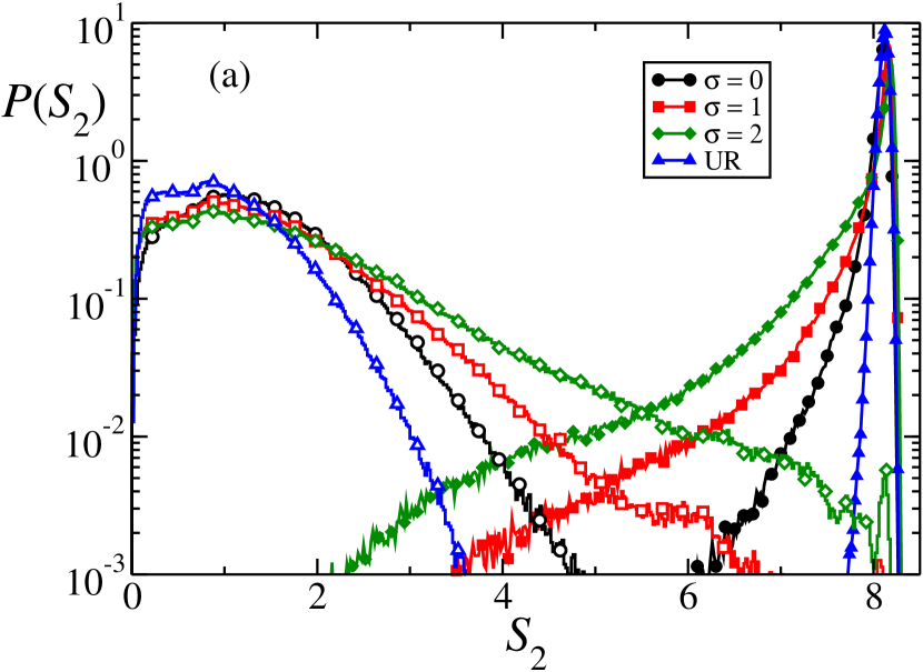
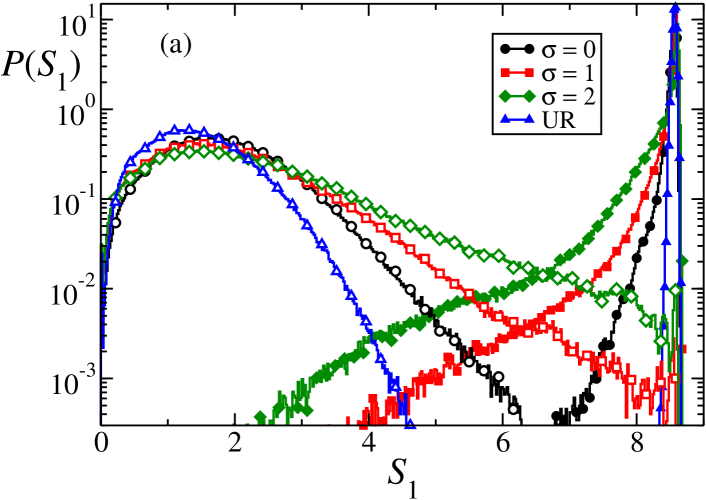
Is it possible to reveal in a more pronounced way the different properties of MBL for UR and speckle disorders in time dynamics? After all those differences were quite strikingly visible in the eigenvector spectral properties was well as in participation entropies. The answer is positive. What we need is a measure of local localization properties, as the broad entropic distributions discussed above convincingly revealed the presence, even in the same sample, of regions seemingly localized to a different degree. Such a measure may be constructed as a local imbalance , involving spins on sites:
| (5) |
The global imbalance is just a sum of . The local imbalances provide information about local scrambling of spin degrees of freedom.
We consider a set of local imbalances at times (in the units) for . Gathering the sets of local imbalances for a large number of disorder realizations we plot the resulting distributions of local imbalance, , in Fig. 8. Consider first the distribution for UR disorder shown in panel (a): for large disorder the distribution is sharply peaked near its maximal unit value indicating an almost complete localization and a good memory of the initial state. On the contrary, for small disorder we observe a smooth gaussian-like profile centered at - a signature of a lost memory of the initial state. With increasing disorder this distribution sharpens, becomes asymmetric (as a total imbalance becomes positive) developing a tail at positive values of . Around a critical disorder value the distribution of is broad reaching the edge at unity. For speckle uncorrelated disorder – Fig. 8(b) – the curves look similar although a careful inspection reveals that for the localized case the tail extending to small is higher than for UR disorder. The broadest distribution, extending almost uniformly between zero and unity is obtained at slightly different value, in comparison to the UR case. The picture changes for the correlated speckle disorder. We observe a spectacular narrowing of distributions in the delocalized case. This may be easily understood, once some disorder value is chosen for a given site, the next correlated site has, with a large probability, a similar disorder value facilitating delocalization. Interestingly the broadest distributions (at values of disorder shifting towards slightly larger values) develop local maxima at showing the abundance of completely delocalized as well as localized local imbalances. Correlated speckle disorder leads thus to the formation of localized and delocalized grains of small size. This behavior becomes even more pronounced at when even for large corresponding globally to the deep MBL case, a noticeable maximum at still exists pointing towards the existence of small regions that locally thermalize.
Note the real resemblance between bimodal distributions observed for local imbalance with the similarly shaped characteristics of the sample averaged gap ratio shown in Fig. 3. The local imbalance allows us to get a similar understanding of the system behavior as eigenvalue statistics not only on the level of the global properties reflected by the imbalance but on a deeper, local level. Let us stress that the measurement of local imbalances requires a single site resolution - however in cold atomic systems as well as in spin models such resolution is already achieved experimentally Gross and Bloch (2017).
V Conclusions
We investigate an optical speckle field placed on top of a quasi one-dimensional optical lattice which allows us to go beyond the continuum approaches considered so far and to model the system within a tight binding description in which the speckle field gives rise to a on-site perturbation. The speckle disorder obtained in that manner has unique features enabling a control over its correlation length. On one hand, the speckle disorder allows us to study MBL transition in an uncorrelated “trully random” disorder, as opposed to the routinely realized experimentally case of quasiperiodic potential which leads to MBL transition of different universality class Khemani et al. (2017). On the other hand, the speckle field opens up the possibility of studying the influence of correlations in disorder on many-body localization transition. A specific exponential distribution function of the uncorrelated speckle already leads to certain differences in the system behavior as compared to usually studied random uniform disorder, the effects become amplified when the speckle correlation length is increased. We observe more pronounced finite size effects that are, surprizingly, hidden in the reduced sensitivity of the system response to changes of its size. This suggests that system sizes of few hundreds sites, available in current experiments in optical lattices may be needed to reach the thermodynamic limit. MBL in the speckle potential has increased sample to sample variation as compared to random uniform disorder, as visualized in the gap ratio analysis as well as in the study of eigenvector properties. With increasing correlations the critical regime of transition broadens.
Additional insights may be obtained from time dynamics. Global imbalance decay confirms the broadening of the transition while a local imbalance, a tool introduced in this work, allows us to visualize the origin of the resistance against localization observed in (particularly correlated) speckle potential. Apparently it favors creation, even for large disorder amplitude, of small grains that locally thermalize. That resembles the behavior expected of rare Griffiths regions for uncorrelated disorder but, surprisingly, the correlations of finite range actually enhance their importance. Excitingly, such local imbalances seem to be readily accessible experimentally offering possible experimental verification of the results presented.
Acknowledgements.
We thank Dominique Delande for providing the code for the speckle potential and discussions. The latter were also enjoyed with Titas Chanda. We acknowledge support by PL-Grid Infrastructure. This research has been supported by National Science Centre (Poland) under projects 2015/19/B/ST2/01028 (P.S. and A.M.), 2018/28/T/ST2/00401 (doctoral scholarship – P.S.) and 2019/35/B/ST2/00034 (J.Z.). Partial support by the Foundation for Polish Science under Polish-French Maria Skłodowska and Pierre Curie Polish-French Science Award is also acknowledged. P.S. acknowledges support by the Foundation for Polish Science (FNP) through scholarship START.Appendix A Appendix
We present here additional numerical results for the model. Those results, while not essential for the conclusions reached in the main text, supplement them with additional numerical evidence.
A.1 Energy dependence of the transition and density of states


The mean gap ratio as a function of the disorder amplitude and the relative energy is presented in Fig. 9. The latter is defined as with being the lowest (highest) eigenvalue for a given disorder realization. We take slices in with size 0.05 obtaining 20 bins for energy. For i.e. an uncorrelated disorder we observe a rather symmetric in energy lobe resembling the one shown in Luitz et al. (2015). The correlation in disorder makes low lying states being more resistant to localization as clearly visible for plot in Fig. 9.
This, at a first glance, surprizing behavior may be partially explained by the energy dependence of the density of states - compare Fig. 10. The raw (unscaled) density is perfectly symmetric with respect to origin. Scaling, performed for each diagonalization separately, shifts slightly the maximum of the density of states to below . For a finite disorder value the maximum of the density concentrates around - that only partially explains the behaviour of the lobe for which, for a correlated disorder has a tip at around .


Still, however, for the maximum of DOS does not corresponds to the lobe in the energy gap ratio observed at . The central part of DOS distribution for scaled eigenenergies [Fig. 10 (b)] is Gaussian for the system with the uniform random and the uncorrelated speckle potential (at least within the range ). For non-zero correlations in the speckle potential the range of DOS with approximately Gaussian distribution decreases with . The non-Gaussian character of DOS distribution is more pronounced for unscaled eigenenergies where for correlated speckle potential the exponential tails are observed.
A.2 Correlations between participation entropy and the sample averaged gap ratio
While in the main text we have shown the participation entropy distributions in different regimes, here we show, compare Fig. 11 that similar picture we obtain for the Shannon entropy . The relatively broad distributions obtained, in particular in the transition regime calls for comparing with gap ratio distributions.


Having in mind the sample-to-sample randomness as exhibited by one may consider the similar properties on the entropy level. Fig. 12 shows the distribution of obtained for disorder realizations with given sample averaged gap ratio , we take . We observe a strong correlation between the center of the distribution of and the value of the sample averaged gap ratio . To quantify those correlations we consider the eigenvectors for 300 eigenvalues around , find their participation entropies and average them for each disorder realization separately. Let as denote such an average of for - sample of values as . The resulting correlation between and sample averaged Shannon entropy is shown in Fig. 13. The correlations are bigger for the speckle than for the random uniform disorder and further increase with the correlation length of the speckle potential. The increase of correlations between the sample averaged quanities and with correlation length can be understood as an effect of diminishing number of uncorrelated random fields in a given disorder sample: for larger values of , the potential fluctuations across a given sample are smaller and hence properties of the sample, reflected either by or , vary less yielding the larger , correlation. For uniform disorder the maximum of the , correlation occurs at the scaled disorder shifting towards for the largest correlation length considered by us. With an increase of the system size the correlation maximum shifts towards higher disorder values. One may speculate that, provided MBL persists in the thermodynamic limit, eventually the maximum shifts towards i.e. the critical point. The dependence of the position of the correlation maximum on system size was checked for systems with to (not shown). It was observed that the shift of the maximum is slower with increasing supporting the observation made for the gap ratio that finite size effects increase with correlation length of the speckle potential.

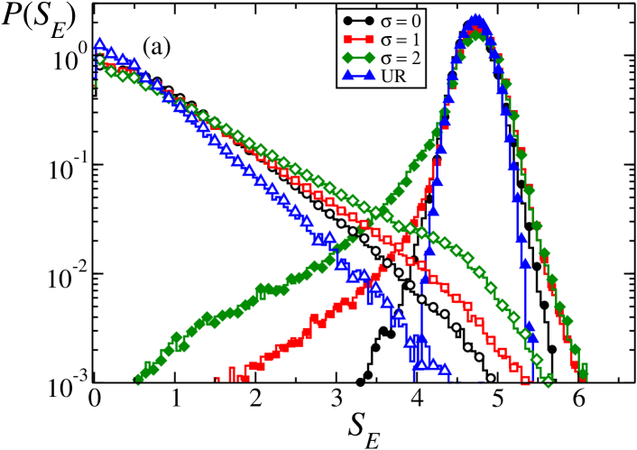

A.3 Bipartite entanglement entropy of eigenstates
To complete the analysis of entropic properties let us consider a different measure, the bipartite entanglement entropy defined as when the system is devided into two parts and . The entanglement entropy is evaluated from Schmidt decomposition as follow
| (6) |
where are singular values obtained from decomposition. The size of the subsystem A over which the partial trace is taken has beens chosen as a half-size of the entire chain, i.e. .
In an analogy to distributions of participation entropy we consider the distributions of entanglement entropy. The results are shown in Fig. 14 for delocalized and localized phase (Fig. 14 (a)), and for transient regime (Fig. 14 (b)).
The behavior of entanglement entropy distributions is qualitatively similar to the ones for participation entropy. The UR potential leads to the Gaussian shape ofentanglement entropy for delocalized phase whereas the distributions for the system with speckle potential become asymmetric with tails that extends towards small region, i.e. there are non-negligible number of values of that correspond to delocalized and localized phases. The overlapped area is increased with increase of correlation length of the speckle potential .
In localized phase the distribution of entanglement entropy seems exponential with the shape independent of the nature of the disorder potential. In this case the slope (in the log scale) of the distribution is maximal for UR potential and is decreasing for speckle potential especially with increase of the speckle correlation length. In the transition regime the distributions are broad and become less sensitive to the correlation length of the speckle potential.
References
- Deutsch (1991) J. M. Deutsch, Phys. Rev. A 43, 2046 (1991).
- Srednicki (1994) M. Srednicki, Phys. Rev. E 50, 888 (1994).
- Rigol et al. (2008) M. Rigol, V. Dunjko, and M. Olshanii, Nature 452, 854 EP (2008).
- D’Alessio et al. (2016) L. D’Alessio, Y. Kafri, A. Polkovnikov, and M. Rigol, Advances in Physics 65, 239 (2016), https://doi.org/10.1080/00018732.2016.1198134 .
- Gornyi et al. (2005) I. V. Gornyi, A. D. Mirlin, and D. G. Polyakov, Phys. Rev. Lett. 95, 206603 (2005).
- Basko et al. (2006) D. Basko, I. Aleiner, and B. Altschuler, Ann. Phys. (NY) 321, 1126 (2006).
- Huse et al. (2014) D. A. Huse, R. Nandkishore, and V. Oganesyan, Phys. Rev. B 90, 174202 (2014).
- Nandkishore and Huse (2015) R. Nandkishore and D. A. Huse, Annual Review of Condensed Matter Physics 6, 15 (2015), https://doi.org/10.1146/annurev-conmatphys-031214-014726 .
- Alet and Laflorencie (2018) F. Alet and N. Laflorencie, Comptes Rendus Physique 19, 498 (2018), quantum simulation / Simulation quantique.
- Abanin et al. (2019) D. A. Abanin, E. Altman, I. Bloch, and M. Serbyn, Rev. Mod. Phys. 91, 021001 (2019).
- Sala et al. (2020) P. Sala, T. Rakovszky, R. Verresen, M. Knap, and F. Pollmann, Physical Review X 10, 011047 (2020).
- Khemani et al. (2020) V. Khemani, M. Hermele, and R. Nandkishore, Phys. Rev. B 101, 174204 (2020).
- Rakovszky et al. (2020) T. Rakovszky, P. Sala, R. Verresen, M. Knap, and F. Pollmann, Physical Review B 101, 125126 (2020).
- Smith et al. (2017) A. Smith, J. Knolle, R. Moessner, and D. L. Kovrizhin, Phys. Rev. Lett. 119, 176601 (2017).
- Brenes et al. (2018) M. Brenes, M. Dalmonte, M. Heyl, and A. Scardicchio, Phys. Rev. Lett. 120, 030601 (2018).
- Magnifico et al. (2020) G. Magnifico, M. Dalmonte, P. Facchi, S. Pascazio, F. V. Pepe, and E. Ercolessi, Quantum 4, 281 (2020).
- Chanda et al. (2020a) T. Chanda, J. Zakrzewski, M. Lewenstein, and L. Tagliacozzo, Phys. Rev. Lett. 124, 180602 (2020a).
- Giudici et al. (2020) G. Giudici, F. M. Surace, J. E. Ebot, A. Scardicchio, and M. Dalmonte, Phys. Rev. Research 2, 032034 (2020).
- Surace et al. (2020) F. M. Surace, P. P. Mazza, G. Giudici, A. Lerose, A. Gambassi, and M. Dalmonte, Phys. Rev. X 10, 021041 (2020).
- Heller (1984) E. J. Heller, Phys. Rev. Lett. 53, 1515 (1984).
- Bogomolny (1988) E. Bogomolny, Physica D 31, 169 (1988).
- Turner et al. (2018) C. J. Turner, A. A. Michailidis, D. A. Abanin, M. Serbyn, and Z. Papić, Nature Physics 14, 745 (2018).
- Ho et al. (2019) W. W. Ho, S. Choi, H. Pichler, and M. D. Lukin, Phys. Rev. Lett. 122, 040603 (2019).
- Khemani et al. (2019) V. Khemani, C. R. Laumann, and A. Chandran, Physical Review B 99, 161101 (2019).
- Iadecola and Žnidarič (2019) T. Iadecola and M. Žnidarič, Phys. Rev. Lett. 123, 036403 (2019).
- Schecter and Iadecola (2019) M. Schecter and T. Iadecola, Phys. Rev. Lett. 123, 147201 (2019).
- Schulz et al. (2019) M. Schulz, C. A. Hooley, R. Moessner, and F. Pollmann, Phys. Rev. Lett. 122, 040606 (2019).
- van Nieuwenburg et al. (2019) E. van Nieuwenburg, Y. Baum, and G. Refael, Proceedings of the National Academy of Sciences 116, 9269 (2019).
- James et al. (2019) A. J. A. James, R. M. Konik, and N. J. Robinson, Phys. Rev. Lett. 122, 130603 (2019).
- Chanda et al. (2020b) T. Chanda, R. Yao, and J. Zakrzewski, Coexistence of localized and extended phases: Many-body localization in a harmonic trap (2020b), arXiv:arXiv:2004:00954 .
- Yao and Zakrzewski (2020a) R. Yao and J. Zakrzewski, Many-body localization of bosons in optical lattice: Dynamics in disorder-free potentials (2020a), arXiv:arXiv:2007.04745 .
- Schreiber et al. (2015) M. Schreiber, S. S. Hodgman, P. Bordia, H. P. Lüschen, M. H. Fischer, R. Vosk, E. Altman, U. Schneider, and I. Bloch, Science 349, 842 (2015).
- Choi et al. (2016) J.-y. Choi, S. Hild, J. Zeiher, P. Schauß, A. Rubio-Abadal, T. Yefsah, V. Khemani, D. A. Huse, I. Bloch, and C. Gross, Science 352, 1547 (2016).
- Khemani et al. (2017) V. Khemani, D. N. Sheng, and D. A. Huse, Phys. Rev. Lett. 119, 075702 (2017).
- Sierant and Zakrzewski (2019) P. Sierant and J. Zakrzewski, Phys. Rev. B 99, 104205 (2019).
- Griffiths (1969) R. B. Griffiths, Phys. Rev. Lett. 23, 17 (1969).
- Vojta (2010) T. Vojta, J. Low Temp. Phys. 161, 299 (2010).
- Agarwal et al. (2015) K. Agarwal, S. Gopalakrishnan, M. Knap, M. Müller, and E. Demler, Phys. Rev. Lett. 114, 160401 (2015).
- Luitz et al. (2015) D. J. Luitz, N. Laflorencie, and F. Alet, Phys. Rev. B 91, 081103 (2015).
- Agarwal et al. (2017) K. Agarwal, E. Altman, E. Demler, S. Gopalakrishnan, D. A. Huse, and M. Knap, Annalen der Physik 529, 1600326 (2017).
- Gopalakrishnan et al. (2016) S. Gopalakrishnan, K. Agarwal, E. A. Demler, D. A. Huse, and M. Knap, Phys. Rev. B 93, 134206 (2016).
- Luitz et al. (2016) D. J. Luitz, N. Laflorencie, and F. Alet, Phys. Rev. B 93, 060201 (2016).
- Luitz and Lev (2017) D. J. Luitz and Y. B. Lev, Annalen der Physik 529, 1600350 (2017).
- Lüschen et al. (2017) H. P. Lüschen, P. Bordia, S. Scherg, F. Alet, E. Altman, U. Schneider, and I. Bloch, Phys. Rev. Lett. 119, 260401 (2017).
- Gopalakrishnan and Parameswaran (2020) S. Gopalakrishnan and S. Parameswaran, Physics Reports 862, 1 (2020), dynamics and transport at the threshold of many-body localization.
- Billy et al. (2008) J. Billy, V. Josse, Z. Zuo, A. Bernard, B. Hambrecht, P. Lugan, D. Clément, L. Sanchez-Palencia, P. Bouyer, and A. Aspect, Nature 453, 891 (2008).
- Piraud and Sanchez-Palencia (2013) M. Piraud and L. Sanchez-Palencia, The European Physical Journal Special Topics 217, 91 (2013).
- Sacha et al. (2009) K. Sacha, C. A. Müller, D. Delande, and J. Zakrzewski, Phys. Rev. Lett. 103, 210402 (2009).
- Delande et al. (2013) D. Delande, K. Sacha, M. Płodzień, S. K. Avazbaev, and J. Zakrzewski, New J. of Phys. 15, 045021 (2013).
- Nandkishore (2014) R. Nandkishore, Phys. Rev. B 90, 184204 (2014).
- Kondov et al. (2015) S. S. Kondov, W. R. McGehee, W. Xu, and B. DeMarco, Phys. Rev. Lett. 114, 083002 (2015).
- De Roeck and Huveneers (2017) W. De Roeck and F. Huveneers, Phys. Rev. B 95, 155129 (2017).
- Mujal et al. (2019) P. Mujal, A. Polls, S. Pilati, and B. Juliá-Díaz, Phys. Rev. A 100, 013603 (2019).
- Mondaini and Rigol (2015) R. Mondaini and M. Rigol, Phys. Rev. A 92, 041601 (2015).
- Sierant et al. (2017) P. Sierant, D. Delande, and J. Zakrzewski, Phys. Rev. A 95, 021601 (2017).
- Sierant and Zakrzewski (2018) P. Sierant and J. Zakrzewski, New Journal of Physics 20, 043032 (2018).
- Orell et al. (2019) T. Orell, A. A. Michailidis, M. Serbyn, and M. Silveri, Phys. Rev. B 100, 134504 (2019).
- Hopjan and Heidrich-Meisner (2020) M. Hopjan and F. Heidrich-Meisner, Phys. Rev. A 101, 063617 (2020).
- Yao and Zakrzewski (2020b) R. Yao and J. Zakrzewski, Phys. Rev. B 102, 014310 (2020b).
- Prelovšek et al. (2016) P. Prelovšek, O. S. Barišić, and M. Žnidarič, Phys. Rev. B 94, 241104 (2016).
- Zakrzewski and Delande (2018) J. Zakrzewski and D. Delande, Phys. Rev. B 98, 014203 (2018).
- Kozarzewski et al. (2018) M. Kozarzewski, P. Prelovšek, and M. Mierzejewski, Phys. Rev. Lett. 120, 246602 (2018).
- Protopopov and Abanin (2019) I. V. Protopopov and D. A. Abanin, Phys. Rev. B 99, 115111 (2019).
- Suthar et al. (2020) K. Suthar, P. Sierant, and J. Zakrzewski, Phys. Rev. B 101, 134203 (2020).
- Bera et al. (2015) S. Bera, H. Schomerus, F. Heidrich-Meisner, and J. H. Bardarson, Phys. Rev. Lett. 115, 046603 (2015).
- Bera et al. (2017) S. Bera, G. De Tomasi, F. Weiner, and F. Evers, Phys. Rev. Lett. 118, 196801 (2017).
- Herviou et al. (2019) L. Herviou, S. Bera, and J. H. Bardarson, Phys. Rev. B 99, 134205 (2019).
- Colmenarez et al. (2019) L. Colmenarez, P. A. McClarty, M. Haque, and D. J. Luitz, SciPost Phys. 7, 64 (2019).
- Goodman (2007) J. Goodman, Speckle Phenomena in Optics: Theory and Applications (Roberts and Co., Englewood, 2007).
- Lugan et al. (2009) P. Lugan, A. Aspect, L. Sanchez-Palencia, D. Delande, B. Grémaud, C. A. Müller, and C. Miniatura, Phys. Rev. A 80, 023605 (2009).
- Oganesyan and Huse (2007) V. Oganesyan and D. A. Huse, Phys. Rev. B 75, 155111 (2007).
- Mehta (1990) M. L. Mehta, Random Matrices (Elsevier, Amsterdam, 1990).
- Haake (2010) F. Haake, Quantum Signatures of Chaos (Springer, Berlin, 2010).
- Sierant et al. (2020a) P. Sierant, M. Lewenstein, and J. Zakrzewski, Polynomially filtered exact diagonalization approach to many-body localization (2020a), arXiv:2005.09534 [cond-mat.dis-nn] .
- Laflorencie et al. (2020) N. Laflorencie, G. Lemarié, and N. Macé, arXiv e-prints , arXiv:2004.02861 (2020), arXiv:2004.02861 [cond-mat.dis-nn] .
- Šuntajs et al. (2020) J. Šuntajs, J. Bonča, T. Prosen, and L. Vidmar, Phys. Rev. B 102, 064207 (2020).
- Chanda et al. (2020c) T. Chanda, P. Sierant, and J. Zakrzewski, Phys. Rev. B 101, 035148 (2020c).
- Šuntajs et al. (2019) J. Šuntajs, J. Bonča, T. Prosen, and L. Vidmar, arXiv e-prints , arXiv:1905.06345 (2019), arXiv:1905.06345 [cond-mat.str-el] .
- Panda et al. (2020) R. K. Panda, A. Scardicchio, M. Schulz, S. R. Taylor, and M. Žnidarič, Europhysics Letters 128, 67003 (2020).
- Sierant et al. (2020b) P. Sierant, D. Delande, and J. Zakrzewski, Phys. Rev. Lett. 124, 186601 (2020b).
- Agrawal et al. (2020) U. Agrawal, S. Gopalakrishnan, and R. Vasseur, Nature Communications 11, 2225 (2020).
- Macé et al. (2019) N. Macé, F. Alet, and N. Laflorencie, Phys. Rev. Lett. 123, 180601 (2019).
- Serbyn et al. (2013) M. Serbyn, Z. Papić, and D. A. Abanin, Phys. Rev. Lett. 111, 127201 (2013).
- Ros et al. (2015) V. Ros, M. Mueller, and A. Scardicchio, Nuclear Physics B 891, 420 (2015).
- Imbrie (2016) J. Z. Imbrie, Phys. Rev. Lett. 117, 027201 (2016).
- Wahl et al. (2017) T. B. Wahl, A. Pal, and S. H. Simon, Phys. Rev. X 7, 021018 (2017).
- Mierzejewski et al. (2018) M. Mierzejewski, M. Kozarzewski, and P. Prelovšek, Phys. Rev. B 97, 064204 (2018).
- Thomson and Schiró (2018) S. J. Thomson and M. Schiró, Phys. Rev. B 97, 060201 (2018).
- Bengtsson and Życzkowski (2006) I. Bengtsson and K. Życzkowski, Geometry of Quantum States (University Press, Cambridge, 2006).
- Fyodorov and Sommers (1995) Y. V. Fyodorov and H.-J. Sommers, Zeitschrift für Physik B Condensed Matter 99, 123 (1995).
- Evers and Mirlin (2000) F. Evers and A. D. Mirlin, Phys. Rev. Lett. 84, 3690 (2000).
- Evers and Mirlin (2008) F. Evers and A. D. Mirlin, Rev. Mod. Phys. 80, 1355 (2008).
- Lukin et al. (2019) A. Lukin, M. Rispoli, R. Schittko, M. E. Tai, A. M. Kaufman, S. Choi, V. Khemani, J. Léonard, and M. Greiner, Science 364, 256 (2019).
- Rispoli et al. (2019) M. Rispoli, A. Lukin, R. Schittko, S. Kim, M. E. Tai, J. Léonard, and M. Greiner, Nature 573, 385 (2019).
- Doggen and Mirlin (2019) E. V. H. Doggen and A. D. Mirlin, Phys. Rev. B 100, 104203 (2019).
- Chanda et al. (2020) T. Chanda, P. Sierant, and J. Zakrzewski, Many-body localization transition in large quantum spin chains: The mobility edge (2020), arXiv:2006.02860 .
- Tal-Ezer and Kosloff (1984) H. Tal-Ezer and R. Kosloff, J. Chem. Phys. 81, 3967 (1984), https://doi.org/10.1063/1.448136 .
- Fehske and Schneider (2008) H. Fehske and R. Schneider, Computational many-particle physics (Springer, Germany, 2008).
- Gross and Bloch (2017) C. Gross and I. Bloch, Science 357, 995 (2017).