Manipulating topological charges via engineering zeros of wave functions
Abstract
Topological charges are typically manipulated by managing their energy bands in quantum systems. In this work, we propose a new approach to manipulate the topological charges of systems by engineering density zeros of localized wave excitations in them. We demonstrate via numerical simulation and analytical analysis that the winding number of a toroidal Bose condensate can be well manipulated by engineering the relative velocities between the dark solitons and their backgrounds. The crossing of relative velocities through zero makes a change in winding number by inducing density zeros during acceleration, with the direction of crossing determining whether charge increases or decreases. Possibilities of observing such winding number manipulation are discussed for current experimental settings. This idea may also be to higher dimensions. These results will inspire new pathways in designing topological materials using quantum simulation platforms.
The stability of topological defects is generally guaranteed by the conservation of their topological charges MerminRMP1979 ; ChaikinCambridge1995 ; KlemanSpringer2003 . In liquid crystals, their stability is determined by the homotopy group of loops surrounding the singularities in the real space StephenRMP1974 ; BallSpringer2017 ; FumeronLCR2023 ; FumeronEPJST2023 . Meanwhile, in recent two decades, the great efforts have been devoted to studying topological defects in the Bloch bands in the momentum space using similar mathematical tools CooperRMP2019 ; ZhangAP2019 ; HasanRMP2010 ; ShenSpringer2017 ; AsbothSpringer2016 . In this way, the topological phase transition can only occur when the conduction and valence bands are closed and reopened at some critical parameters, and in the topological phase, the bulk-edge correspondence ensures the emergence of edge states HasanRMP2010 ; ShenSpringer2017 ; AsbothSpringer2016 . The search for various topological phases and their potential application in topological quantum computation remains one of the most important themes in condensed matter physics and quantum simulation HasanRMP2010 ; ShenSpringer2017 ; AsbothSpringer2016 ; NayakRMP2008 ; BulutaRPP2011 ; BlochNP2012 ; GrossSince2017 ; TerhalRMP2015 ; TokuraNRP2019 . In experiments, the topology of bands can well explain the quantum Hall effect HeNSR2014 ; KlitzingNRP2020 ; ChangRMP2023 , Thouless pumping CitroNRP2023 ; NakajimaNP2016 ; LohseNP2016 ; JurgensenNature2021 , quantized Hall drifts AidelsburgerNP2015 ; ZhuSince2023 , and other topological phenomena in terms of the Berry curvature Berry1984 ; XiaoRMP2010 .
The robustness of topological phases implies that it is hard to engineer the topological charges without destroying the geometry of the manifolds ShenSpringer2017 ; AsbothSpringer2016 ; XiaoRMP2010 ; RachelRPP2018 ; DingNRP2022 . This general conclusion also means that we can engineer the topological charges by controlling the singularities in the manifolds. These singularities correspond to the touches of conduction and valence bands of the Bloch bands or the zeros of wave functions ShenSpringer2017 ; AsbothSpringer2016 ; XiaoRMP2010 . As we have shown in Refs. ZhaoPRE2021 ; WangPS2024 , the zeros of wave functions carries the nonzero topological charges in real space, which can be transferred to the system under consideration if they are carefully designed. As a central idea of this work, we expect that engineering the zeros of wave functions could provide an alternative approach for manipulating topological charges.
This Letter reports the manipulation of topological charges in a toroidal Bose condensate by engineering the zeros of wave functions. The major idea is that the acceleration motion of dark solitons usually involves the density zeros ZhaoPRA2020 ; MengJPB2024 , which can be used to manipulate the topology of the condensate. To this end, we consider one or more dark solitons imprinted on a ring-shaped condensate and demonstrate that the topological charge, characterized by its winding number, can be manipulated by controlling the relative velocities between the solitons and their background density currents through accelerating the solitons. We propose two protocols for accelerating dark solitons: loading (I) impurity atoms or (II) bright solitons in dark solitons and applying weak forces on them. These protocols can address the challenges of directly accelerating dark solitons due to their backgrounds. Each crossing of the zero relative velocities (corresponding to the emergence of density zeros) induces a abrupt change in the winding number, with the direction of crossing determining whether winding number increases or decreases. We further show that accelerating (III) multiple dark solitons provides diverse techniques for tailoring topological charges. This idea may be used to engineer the topology of the Bloch bands, leading to the control of the associated edge states.
Physical Model: We use a binary toroidal Bose condensate as platform to demonstrate our idea. After rescaling the atomic mass and Planck’s constant to be , the dimensionless mean-field energy of system in polar coordinates can be expressed as DalfovoRMP1999 ; PitaevskiiOUPress2016
| (1) |
where and represent the dark solitons and localized waves components, respectively. The localized waves (either impurity atoms or bright solitons) are trapped by dark solitons through the nonlinear interaction . The dimensionless paraments , and represent the corresponding interaction strengths among atoms. To avoid snaking instability CarreteroNonlinearity2008 ; FrantzeskakisJPA2010 , the trapping frequency must be sufficiently large along the radial direction , making the condensate appearing as a quasi-one-dimensional ring along the angular direction . The forces acting on the localized waves can accelerate the dark solitons without modifying their background density, which provides a good protocol for controlling the motions of dark solitons ZhaoPRA2020 ; MengJPB2024 . Hereafter, we set the radius of the toroidal condensate to . In the following, we present three different strategies for manipulating the topological charges of the condensate.
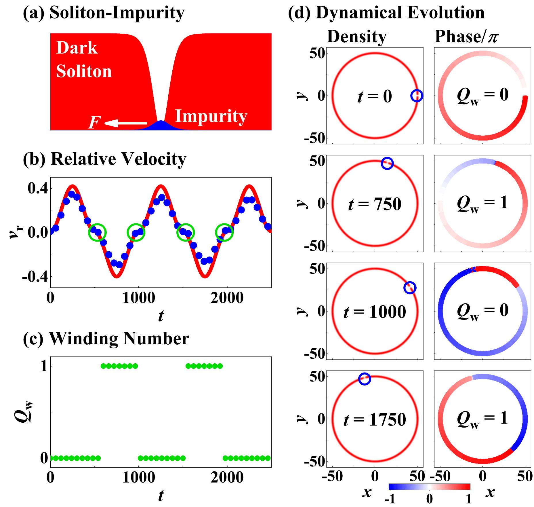
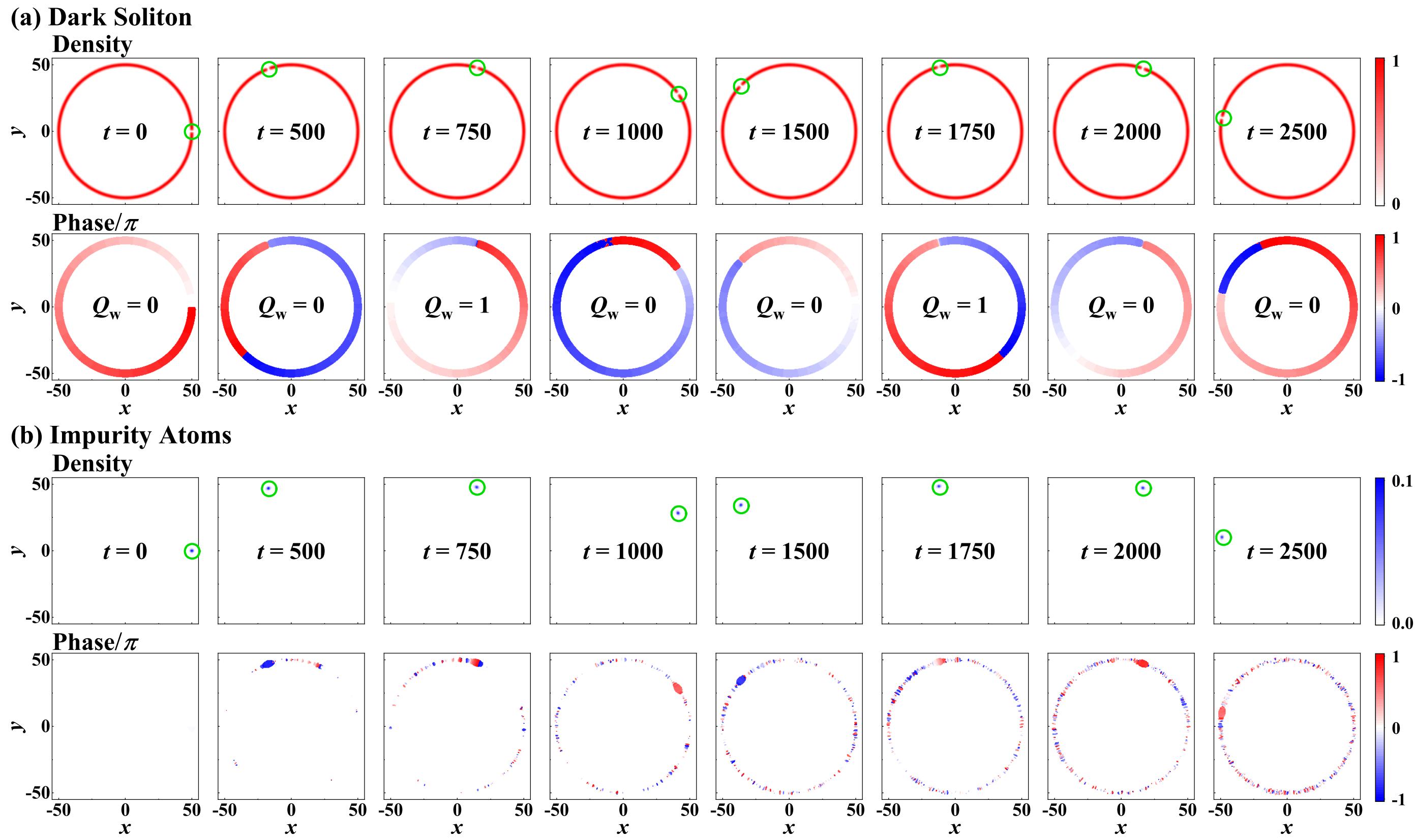
(I): We consider a dark soliton coupled with some impurity atoms, where the impurity atoms are driven by a weak force , as shown in Fig. 1 (a). For convenience, we replace the localized wave with to account for the impurity atoms. The initial wave function of these two components can be expressed as MengNJP2023 ; MengJPB2024
| (2a) | |||
| (2b) | |||
In the above states, is the toroidal ground state of the condensate, which can be obtained through the imaginary-time evolution method YangSIAM2010 ; BaoKRM2013 ; BaoJCP2003 ; ChiofaloPRE2000 ; LehtovaaraJCP2007 by solving the two-dimensional Gross-Pitaevskii (GP) equations, assuming that two components admit the same density. The parameters , and represent the soliton velocity, background density velocity, and sound speed, respectively. Therefore, signifies the relative velocity between the soliton and background density. Seeing Eq. (2), we can easily check that when is sufficiently large, while .
The phase jump of dark soliton is given by with , and . Notably, when , occurs at , yielding the zero of dark soliton, which is essential for its phase jump. In this way, the topological phase transition can only occur when the relative velocity . During the evolution of GP equations, the profiles of two components can still be described by Eq. (2), with and being time-dependent, thus can still be employed to identify the phase transition and the associated phase jump of dark soliton. Furthermore, the single-valued nature of the order parameter requires that the phase variations along the ring should satisfy BrandJPB2001 ; MateoPRA2015 ; ShamailovPRA2019
| (3) |
where represents the phase shift induced by the background density current; see Eq. (2a). The integer signifies the winding number of toroidal condensate, which can be defined as the number of times the phase winds through in a closed loop counterclockwise around the ring. In recent experiments RyuPRL2007 ; RamanathanPRL2011 ; WrightPRL2013 ; RyuPRL2013 ; EckelNature2014 , the winding number can only be manipulated by a rotating weak link in the absence of dark solitons, which is by changing ; however, an easier way to achieve this is by changing , see below.
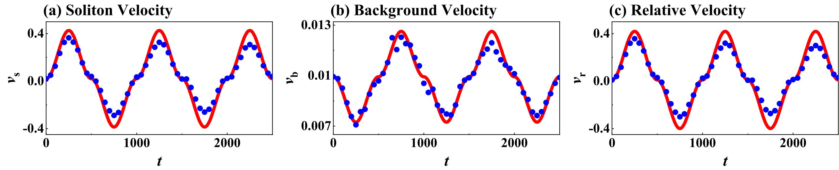
We present our numerical results employing the Fourier pseudo-spectral method YangSIAM2010 ; BaoKRM2013 ; BaoJCP2003 with the Strang splitting scheme to solve the GP equations in Fig. 1. The initial parameters for this our simulation are and , and the weak force is designed as , where denotes the floor function. Since dark soliton admits a negative inertial mass, its acceleration is directed opposite to the direction of weak force MengNJP2023 ; FrantzeskakisJPA2010 ; MengJPB2024 ; AycockPNAS2017 ; HurstPRA2017 . The density and phase of dark soliton at various moments are shown in Fig. 1 (d), and the detailed dynamical evolutions of the dark soliton and impurity atoms are presented in Sec. SI of Supplemental Material (SM), which includes a video representation. The positions of the dips in the dark soliton are monitored to determine while the phase gradient of the background density enables the determination of , allowing for the identification of . The winding number can be obtained by integrating the phase gradient of the condensate along the ring. The evolution of and are depicted in Fig. 1 (b) and (c), respectively. Our results demonstrate that the density zero occurs at , precisely corresponding to the abrupt jump points of . Moreover, the crossing direction of the zero relative velocity determines whether the winding number increases or decreases. As previously mentioned, the profiles of the two components can still be described by Eq. (2) during evolution, which enables us to theoretically describe the evolution of the soliton by quasiparticle theory using the Lagrangian variational method (see Sec. SII of SM for details). As depicted in Fig. 1 (b), the results given by quasiparticle theory agree with those of numerical simulation.
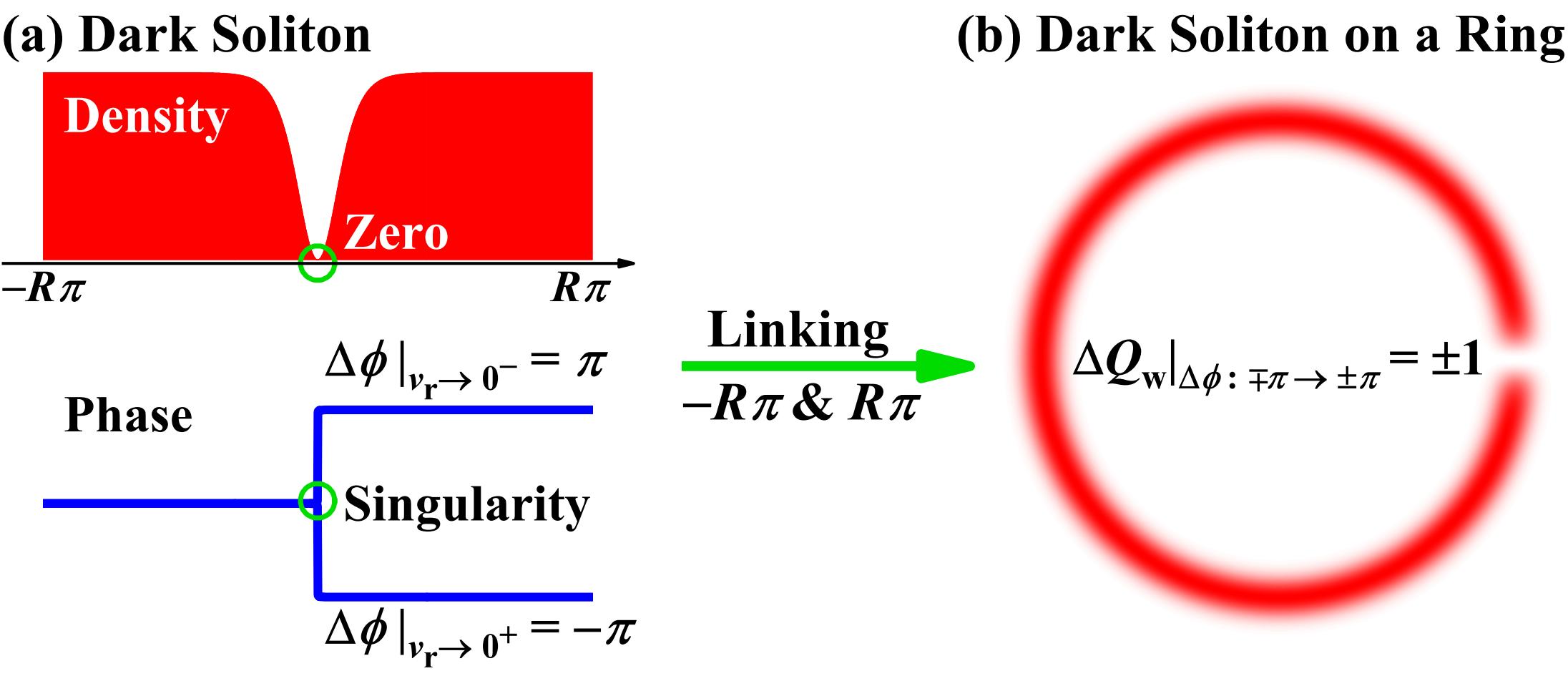
In Refs. ZhaoPRE2021 ; WangPS2024 , we have shown that the wave function admits a phase jump of at the density zero, with the sign determined by the approach direction. For one dark soliton, we find that
| (4) |
Therefore, as the zero relative velocity is approached from different directions, the phase jump direction varies. For instance, when changes from a positive value to zero, a phase jump of occurs; and when changes from zero to a negative value, a phase jump of occurs; then a total phase jump of occurs, as demonstrated in Fig. 2 (a); and vice versa. In one-dimensional settings with open boundaries, this phase jump occurs in accelerating dark soliton but is not observable. Linking the two ends of a one-dimensional dark soliton to form a ring configuration, we uncover a significant finding. As derived from Eq. (3), a phase jump induced by the crossing of zero relative velocity brings a change of in the winding number , as demonstrated in Fig. 2 (b). Explicitly, each crossing of zero relative velocity induces a change in the winding number, with the direction of the crossing determining whether the winding number increases or decreases.
The density zeros of wave functions have deep origins in physics. These singularities induce the emergence of nonintegrable phase factors in certain parameter spaces, with the integration encircling these singularities typically yielding a nonzero topological phase. This idea can even be traced back to Dirac’s work on monopoles DiracPRSLA1931 , wherein the relation between nonintegrable phases and the integer topological magnetic charges. Furthermore, Nye and Berry pointed out that the wave dislocations in wave systems correspond to the zeros of wave functions, and the phase singularities play essential roles in many striking phenomena in wave physics NyePRSLA1974 ; BerryLSA2023 . The dynamics of zeros are also closely related with the topological properties of physical systems DuanPRE1999 ; DuanPRE199960 , such as quantifying the spatiotemporal behavior of spiral wave by tracking phase singularities ZhangCPL2007 ; LiPRE2018 ; HePRE2021 . These results, together with the results presented in this work, suggest that the zeros of wave functions have the profound implications for physics.
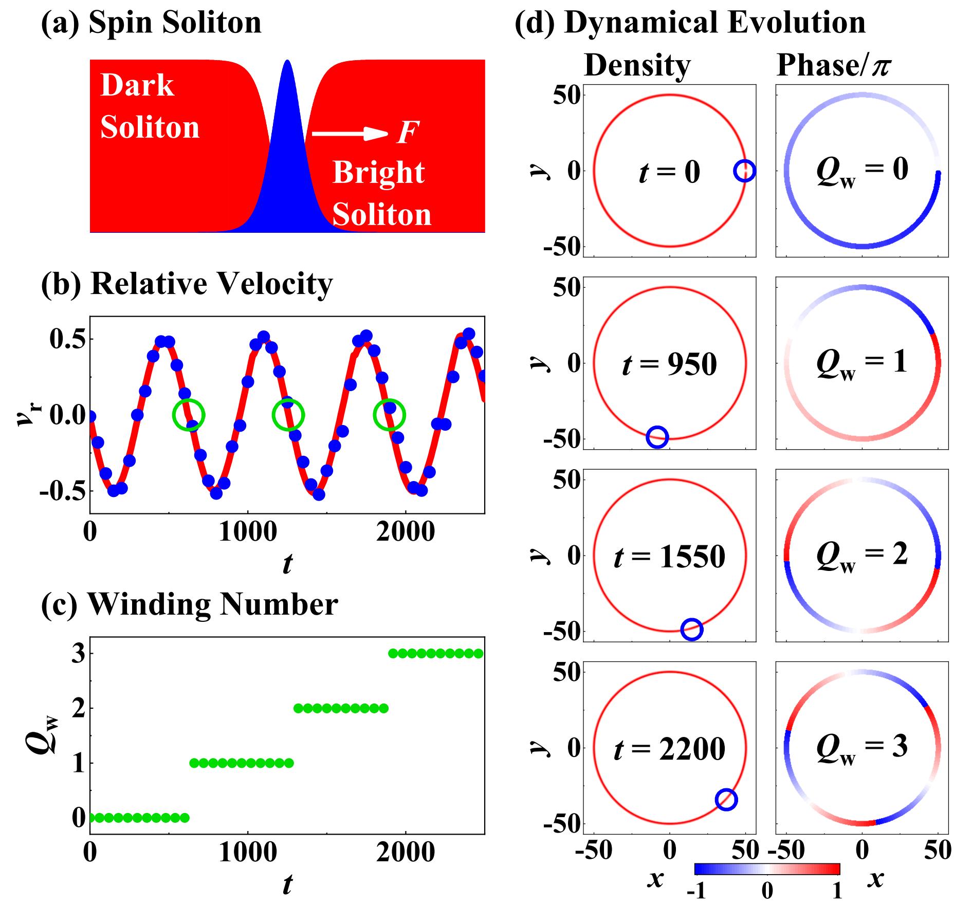
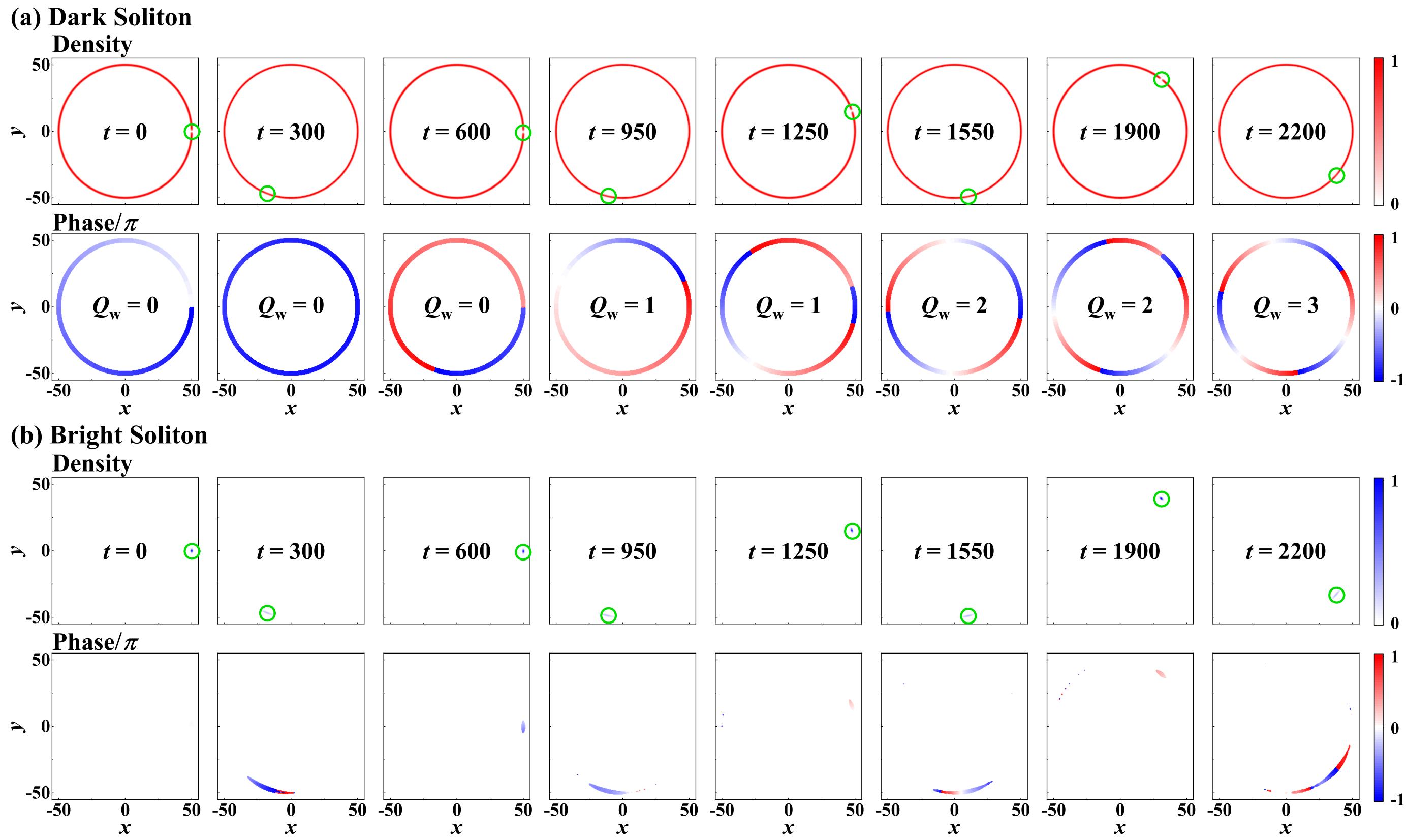
(II): The above protocol can only realize two states, characterized by the winding number of . This limitation prompts us to consider a more general question: can we manipulate the winding number to a arbitrary integer number? In following, we propose a feasible protocol to progressively increase or decrease winding number based on the oscillation of the spin soliton driven by a weak constant force ZhaoPRA2020 ; MengPRA2022 ; MengCNSNS2022 , as shown in Fig. 3 (a). Here, we replace the localized wave with the bright soliton and set . The initial wave function of these two components can be expressed as ZhaoPRA2020 ; MengPRA2022
| (5a) | |||
| (5b) | |||
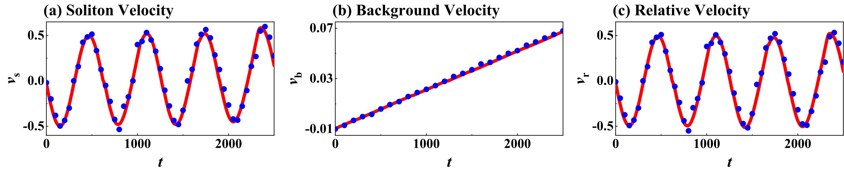
where , which is related to the velocity limit of spin soliton MengPRA2022 . The basic characteristic of spin soliton admits a uniform total density , as shown in Fig. 3 (a). Applying a weak constant force on bright soliton and setting initial parameters as and , we perform numerical simulation and results are shown in Fig. 3. The density and phase of dark soliton at various moments are shown in Fig. 3 (d), and the detailed dynamical evolutions of the dark and bright solitons are presented in Sec. SI of SM, which includes a video representation. We find that that the relative velocity exhibits a periodic oscillation, which corresponds to the ac oscillation induced by periodic transition between negative and positive inertial mass ZhaoPRA2020 ; MengPRA2022 ; MengCNSNS2022 . Notably, density zero only emerges when the relative velocity crosses zero from positive to negative values, as pointed by the green circles in in Fig. 3 (b), where the spin soliton admits the negative inertial mass. There is no density zero for inverse crossing direction, which is due to different properties of spin solitons with different inertial masses ZhaoPRA2020 ; MengPRA2022 ; MengCNSNS2022 . Therefore, the dark soliton does admit the density zero at zero relative velocity in the same manner, which leads to a step-like increment in the winding number , as presented in Fig. 3 (c). Also, as depicted in Fig. 3 (b), the results given by quasiparticle theory (see Sec. SII of SM for details) agree with those of numerical simulation. However, it should be emphasized that the system may become unstable and eventually break when the winding number reaches very high values with the increment of background density velocity . For the parameters used in Fig. 3, the maximum observed value for is approximately .
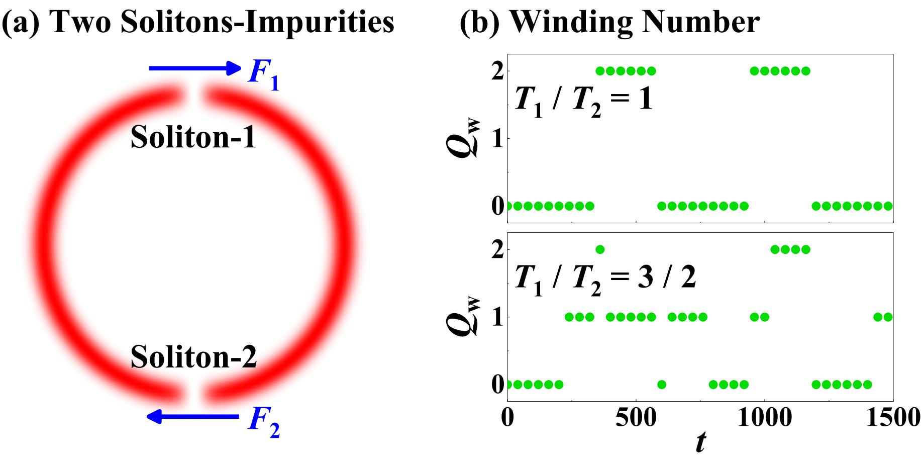
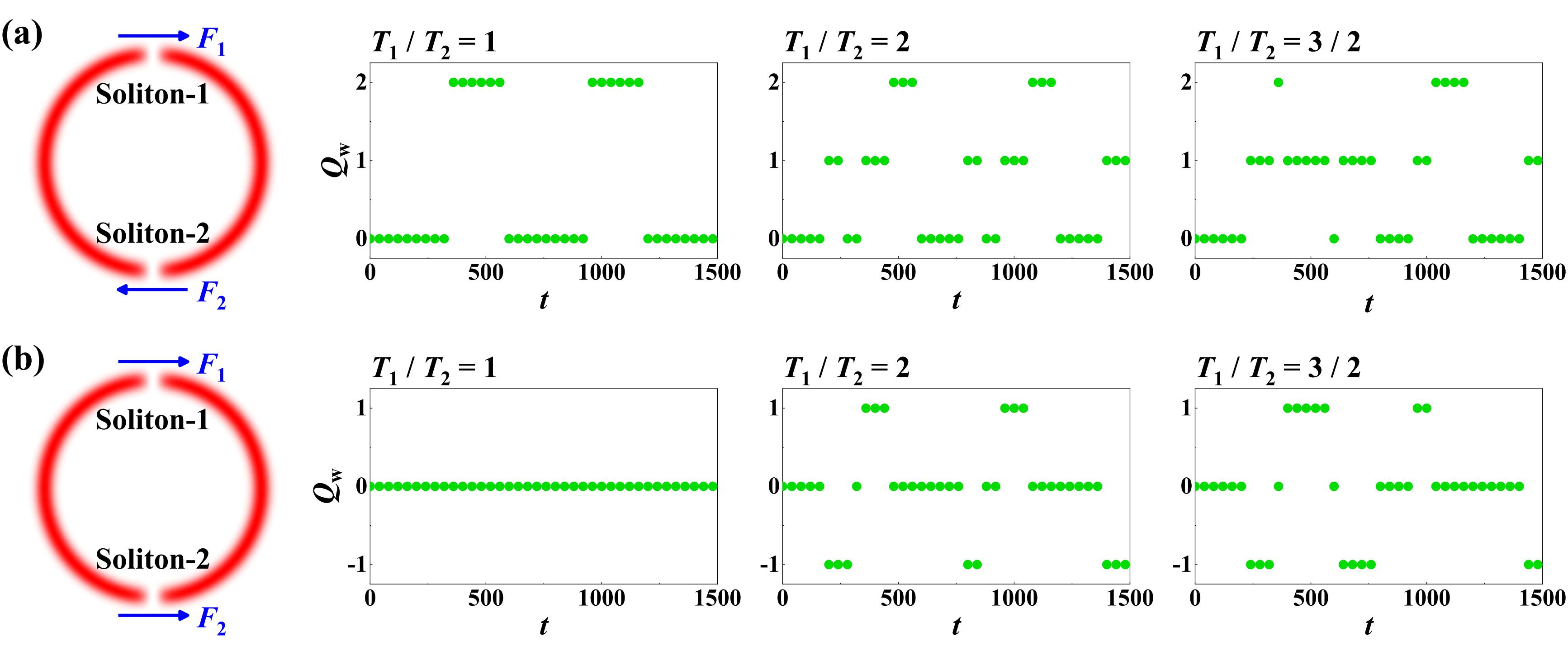
(III): We investigate two well-separated dark solitons with coupling impurity atoms driven by two weak force , as shown in Fig. 4 (a), which can be used as a platform to demonstrate the arbitrary tunability of winding number. The initial states for two dark solitons and coupled impurities are described by and with . Each soliton-impurity is driven by a weak force . We present different evolution of winding number by adjusting period ratio in Fig. 4 (b). When , the winding number jumps two times of the case of one dark soliton (see in in Fig. 1 (c)); when , the winding number evolves in a near random way due to the different frequencies and directions of the density zero crossings. More manipulations of winding number and cases involving multiple spin solitons are provided in Sec. SIII of SM.
Experimental Observation: Finally, we discuss the possibilities to observe the winding number manipulations in real experiments. Let’s consider a Bose condensate with two internal states HallPRL1998 ; MertesPRL2007 ; BeckerNP2008 to observe the results presented in Fig. 1. The related scattering lengthes are about ( being the Bohr radius) HallPRL1998 ; MertesPRL2007 . The condensate can be loaded in a toroidal optical dipole trap RyuPRL2007 ; RamanathanPRL2011 ; WrightPRL2013 ; RyuPRL2013 ; EckelNature2014 with radial and vertical trapping frequencies of and a radius of . The initial states can be prepared well by imprinting a dark soliton with atoms (the background density of ) in state and filling the density dip with atoms in state FrantzeskakisJPA2010 ; BeckerNP2008 . The effective radial length is with healing length of . A weak uniform gradient magnetic field can be applied along the angle coordinate as the effective force to drive atoms LuoSR2016 . By setting a sinusoidal modulating gradient magnetic field LuoSR2016 ; AnnalaPRR2024 ; RayNature2014 ; RayScience2015 with peak gradient of and period of , one can observe 2 times winding number jumps within the time duration of . The predictions in this work could be realized through the state-of-the-art experimental techniques.
Conclusion and Discussion: To conclude, we demonstrate that the topological charge of a toroidal Bose condensate can be well manipulated by engineering its density zeros. When the relative velocities between the dark solitons and their background density currents are zeros, the density zeros occur. In our schemes, loading and driving dark solitons open up the possibility of manipulating winding number, which provides a new approach for quantum computation, quantum simulation, and other quantum-based applications NayakRMP2008 ; BulutaRPP2011 ; BlochNP2012 ; GrossSince2017 ; TerhalRMP2015 ; TokuraNRP2019 ; AmicoRMP2022 ; PoloQT2024 .
Further, vortices, as fundamental topological excitations in high-dimensional systems, also admit the presence of density zeros and their charges determine the topology of systems PitaevskiiOUPress2016 ; FetterRMP2009 ; MatthewsPRL1999 ; LeanhardtPRL2002 . The higher-order vortices exhibit distinctive properties of density zeros compared with fundamental ones ShinPRL2004 ; IsoshimaPRL2007 ; LanPRL2023 . We expect that the charges of various vortices can be well manipulated through engineering the density zeros. These results could inspire new pathways in the design of topological systems by engineering the zeros of localized waves.
This work is supported by the National Natural Science Foundation of China (Contracts No. 12375005, No. 12235007 and No. 12247103) and the Major Basic Research Program of Natural Science of Shaanxi Province (Grant No. 2018KJXX-094).
SM A: Dynamical Evolutions of Solitons
In order to visualize the dynamics of soliton in Figs. 1 and 3 in main text more clearly, we provide the dynamical evolutions of soliton driven by a weak force in a toroidal Bose condensate at various moments (see the videos for more details).
.1 Densities and Phases Evolutions of Soliton-Impurity System
We provide the density and phase evolution of a dark soliton with impurity atoms driven by a weak force , as shown in Fig. 5. We set the weak force as and soliton relative velocity as (with soliton velocity and background density velocity ), where the parameters are the same as those in Fig. 1 in main text. When a weak force applies on the impurity atoms trapped in the dark soliton, the direction of acceleration of dark soliton is in the opposite direction of force due to its negative mass effect MengNJP2023 ; MengJPB2024 . Therefore, the dark soliton will initially move in a counterclockwise direction and tend towards zero relative velocity. Subsequently, dark soliton will move in a clockwise direction and reverse its relative velocity direction due to the reversal of direction of force . This process will be repeated accordingly, as indicated by the green circles markers in Fig. 5. Explicitly, each crossing of zero relative velocity induces a change in the winding number, with the direction of the crossing determining whether the winding number increases or decreases.
.2 Densities and Phases Evolutions of Spin Soliton
We provide the density and phase evolution of a spin soliton driven by a weak force , as shown in Fig. 6. We set the weak force as and soliton relative velocity as (with soliton velocity and background density velocity ), where the parameters are the same as those in Fig. 3 in main text. When a weak constant force applies on the bright soliton trapped in the dark soliton, the spin soliton exhibits a periodic oscillation due to the negative-positive mass transition ZhaoPRA2020 ; MengPRA2022 . Thus the spin soliton will initially move in a clockwise direction and then move in a counterclockwise direction. This process will be repeated accordingly, as indicated by the green circles markers in Fig. 6. Notably, the density zero only emerges when the relative velocity crosses zero from positive to negative values, where spin soliton admits the negative inertial mass ZhaoPRA2020 ; MengPRA2022 . Therefore, the continuous crossing of zero relative velocity in the same manner induces a step-like increment in the winding number .
SM B: Derivation of Quasiparticle Description
The profiles of solitons in two components admit certain particle properties during evolution, which provide possibilities to theoretically describe the evolution of solitons by quasiparticle theory using the Lagrangian variational method.
.3 Quasiparticle Description of Soliton-Impurity System
Considering a dark soliton coupled with some impurity atoms along the ring, the dynamics of quasi-one-dimensional coupled system can be described by
| (6a) | ||||
| (6b) | ||||
We try to use the Lagrangian variational method to evaluate the dynamics of solitons by introducing the following trial wavefunctions (taking ) MengNJP2023 ; MengJPB2024
| (7a) | ||||
| (7b) | ||||
where accounts for the depth of dark soliton, for its width, and for its position angle. Considering the single-valued order parameter whenever a closed loop is followed, we need introduce the continuity condition . Then the Lagrangian of the system can be written as
| (8) |
where . It is now straightforward to apply the Euler-Lagrangian equation , where . Solving them, the most essential relations for soliton motion can be derived as follows
| (9) |
and
| (10) |
where and denotes the particle number of impurity atoms. In order to describe the evolution of solitons in Fig. 1 of main text, we firstly numerically calculate from Eq. (9); then, we can obtain the soliton velocity from Eq. (10). The background density velocity can be calculated through . Thus, we can directly get the relative velocity , which is presented as the red lines in Fig. 1 (b) of main text. As shown in Fig. 7, results of quasiparticle theory are in agree with those of numerical simulation.
.4 Quasiparticle Description of Spin Soliton
Considering a spin soliton along the ring, the dynamics of quasi-one-dimensional coupled system can be given by
| (11a) | ||||
| (11b) | ||||
We try to use the Lagrangian variational method to evaluate the dynamics of soliton by introducing the following trial wavefunctions (taking ) ZhaoPRA2020 ; MengPRA2022
| (12a) | ||||
| (12b) | ||||
where accounts for the depth of dark soliton, for its width, and for its position angle. Considering the single-valued order parameter whenever a closed loop is followed, we need introduce the continuity condition . Then the Lagrangian of the system can be written as
| (13) | |||||
where . It is now straightforward to apply the Euler-Lagrangian equation , where . Solving them, the most essential relations for soliton motion can be derived as follows
| (14) |
and
| (15) |
where denotes the particle number of bright solitons. In order to describe the evolution of solitons in Fig. 3 of main text, we firstly numerically calculate from Eqs. (14) and (15); then, we can obtain the soliton velocity from Eq. (14). The background density velocity can be calculated through . Thus, we can directly get the relative velocity , which is presented as the red lines in Fig. 3 (b) of main text. As shown in Fig. 8, results of quasiparticle theory are in agree with those of numerical simulation.
SM C: Weak Force-Driven Multiple Dark Solitons Protocol for Manipulating Winding Number
We would like to further discuss the abundant manipulations of winding number by considering more solitons in a toroidal Bose condensate.
.5 Weak Force-Driven Two Solitons in Solitons-Impurities System
Considering two well-separated dark solitons coupled with impurity atoms, the initial states can be expressed as
| (16) | |||||
| (17) |
Two solitons-impurities are driven by the sinusoidal driving forces and , respectively. The amplitudes of force are set to in Fig. 9 (a) and in Fig. 9 (b), respectively. One can investigate different evolutions of winding numbers by adjusting the periodic rate . For , the winding number jumps two times that of the one dark soliton (see in Fig. 1 in in main text) when ; or there are no change for winding number when . For , the winding number will evolve in a near random way due to the different frequencies and directions of the density zero crossings, when both .
.6 Weak Force-Driven Two Spin Solitons
Considering two well-separated spin solitons, the initial states can be expressed as
| (18) | |||||
| (19) |
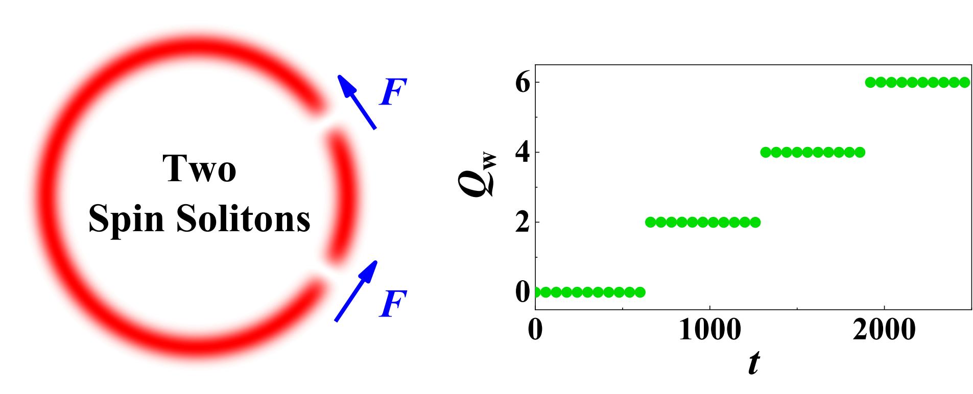
Two spin solitons are both driven by a weak constant force . One can see that the winding number jumps two times that of the one spin soliton in the step-like behavior (see in Fig. 3 in in main text), as shown in Fig. 10. More manipulation of winding number can be realized by involving multiple spin solitons.
References
- (1) N. D. Mermin, The topological theory of defects in ordered media, Rev. Mod. Phys. 51, 591 (1979).
- (2) P. M. Chaikin and T. C. Lubensky, Principles of Condensed Matter Physics, (Cambridge University Press, Cambridge, 1995).
- (3) M. Kleman and O. D. Lavrentovich, Soft Matter Physics, (Springer, New York, 2003).
- (4) M. J. Stephen and J. P. Straley, Physics of liquid crystals, Rev. Mod. Phys. 46, 617 (1974).
- (5) J. M. Ball, E. Feireisl, F. Otto, Mathematical Thermodynamics of Complex Fluids, (Springer, Cham, 2017).
- (6) S. Fumeron, B. Berche, and F. Moraes, Geometric theory of topological defects: methodological developments and new trends, Liq. Crys. Rev. 9, 85 (2023).
- (7) S. Fumeron and B. Berche, Introduction to topological defects: from liquid crystals to particle physics Eur. Phys. J. Spec. Top. 232, 1813 (2023).
- (8) N. R. Cooper, J. Dalibard, and I. B. Spielman, Topological bands for ultracold atoms, Rev. Mod. Phys. 91, 015005 (2019).
- (9) D. W. Zhang, Y. Q. Zhu, Y. X. Zhao, H. Yan, and S. L. Zhu, Topological quantum matter with cold atoms, Adv. Phys. 67, 253 (2019).
- (10) M. Z. Hasan and C. L. Kane, Colloquium: Topological insulators, Rev. Mod. Phys. 82, 3045 (2010).
- (11) S. Q. Shen, Topological Insulators, (Springer, Singapore, 2017).
- (12) J. K. Asbóth , L. Oroszlány , and A. Pályi A Short Course on Topological Insulators, (Springer, Cham, 2016).
- (13) C. Nayak, S. H. Simon, A. Stern, M. Freedman, and S. D. Sarma, Non-Abelian anyons and topological quantum computation, Rev. Mod. Phys. 80, 1083 (2008).
- (14) I. Buluta, S. Ashhab, and F. Nori, Natural and artificial atoms for quantum computation, Rep. Prog. Phys. 74, 104401 (2011).
- (15) I. Bloch, J. Dalibard and S. Nascimbène, Quantum simulations with ultracold quantum gases, Nat. Phys. 8, 267 (2012).
- (16) C. Gross, I. Bloch, Quantum simulations with ultracold atoms in optical lattices, Science 357, 995 (2017).
- (17) B. M. Terhal, Quantum error correction for quantum memories, Rev. Mod. Phys. 87, 307 (2015).
- (18) Y. Tokura, K. Yasuda and A. Tsukazaki, Magnetic topological insulators, Nat. Rev. Phys. 1, 126 (2019).
- (19) K. He, Y. Y. Wang, and Q. K. Xue, Quantum anomalous Hall effect, Nat. Sci. Rev. 1, 38 (2014).
- (20) K. von Klitzing, T. Chakraborty, P. Kim, V. Madhavan, X. Dai, J. McIver, Y. Tokura, L. Savary, D. Smirnova, A. M. Rey, C. Felser, J. Gooth, and X. L. Qi, 40 years of the quantum Hall effect, Nat. Rev. Phys. 2, 397 (2020).
- (21) C. Z. Chang, C. X. Liu, and A. H. MacDonald, Colloquium: Quantum anomalous Hall effect, Rev. Mod. Phys. 95, 011002 (2023).
- (22) R. Citro and M. Aidelsburger, Thouless pumping and topology, Nat. Rev. Phys. 5, 87 (2023).
- (23) S. Nakajima, T. Tomita, S. Taie, T. Ichinose, H. Ozawa, L. Wang, M. Troyer and Y. Takahashi, Topological Thouless pumping of ultracold fermions, Nat. Phys. 12, 296 (2016).
- (24) M. Lohse, C. Schweizer, O. Zilberberg, M. Aidelsburger and I. Bloch, A Thouless quantum pump with ultracold bosonic atoms in an optical superlattice, Nat. Phys. 12, 350 (2016).
- (25) M. Jürgensen, S. Mukherjee and M. C. Rechtsman, Quantized nonlinear Thouless pumping, Nature 596, 63 (2021).
- (26) M. Aidelsburger, M. Lohse, C. Schweizer, M. Atala, J. T. Barreiro, S. Nascimbène, N. R. Cooper, I. Bloch and N. Goldman, Measuring the Chern number of Hofstadter bands with ultracold bosonic atoms, Nat. Phys. 11, 162 (2015).
- (27) Z. J. Zhu, M. Gä chter, A. S. Walter, K. Viebahn and T. Esslinger, Reversal of quantized Hall drifts at noninteracting and interacting topological boundaries, Science 384, 317 (2024).
- (28) M. V. Berry, Quantal phase factors accompanying adiabatic changes, Proc. R. Soc. Lond. A 392, 45 (1984).
- (29) D. Xiao, M. C. Chang, and Q. Niu, Berry phase effects on electronic properties, Rev. Mod. Phys. 82, 1959 (2010).
- (30) S. Rachel, Interacting topological insulators: a review, Rep. Prog. Phys. 81, 116501 (2018).
- (31) K. Ding, C. Fang, and G. C. Ma, Non-Hermitian topology and exceptional-point geometries, Nat. Rev. Phys. 4, 745 (2022).
- (32) L. C. Zhao, Y. H. Qin , C. Lee, J. Liu, Classification of dark solitons based on topological vector potentials, Phys. Rev. E 103, L040204 (2021).
- (33) B. H. Wang, N. Mao, L. C. Zhao, The complete set of eigenstates in one type of N-multiple quantum wells, Phys. Scr. 99, 035108 (2024).
- (34) L. C. Zhao, W. L. Wang, Q. L. Tang, Z. Y. Yang, W. L. Yang, and J. Liu, Spin soliton with a negative-positive mass transition, Phys. Rev. A 101, 043621 (2020).
- (35) L. Z. Meng, L. C. Zhao, T. Busch and Y. P. Zhang, Controlling dark solitons on the healing length scale, J. Phys. B: At. Mol. Opt. Phys. 57, 145302 (2024).
- (36) F. Dalfovo, S. Giorgini, L. P. Pitaevskii, and S. Stringari, Theory of Bose-Einstein condensation in trapped gases, Rev. Mod. Phys. 71, 463 (1999).
- (37) L. Pitaevskii and S. Stringari, Bose-Einstein Condensation and Superfluidity, (Oxford University Press, Oxford, 2016).
- (38) R. Carretero-González, D. J. Frantzeskakis, and P. G. Kevrekidis, Nonlinear waves in Bose-Einstein condensates: physical relevance and mathematical techniques, Nonlinearity 21, R139 (2008).
- (39) D. J. Frantzeskakis, Dark solitons in atomic Bose-Einstein condensates: from theory to experiments, J. Phys. A: Math. Theor. 43, 213001 (2010).
- (40) L. Z. Meng, N. Mao, and L. C. Zhao, The dispersion relation of a dark soliton, New J. Phys. 25, 043015 (2023).
- (41) J. K. Yang, Nonlinear Waves in Integrable and Nonintegrable Systems, (SIAM, Philadelphia, 2010).
- (42) W. Z. Bao, and Y. Y. Cai, Mathematical theory and numerical methods for Bose-Einstein condensation, Kinet. Relat. Models 6, 1 (2013).
- (43) W. Z. Bao, D. Jaksch, and P. A. Markowich, Numerical solution of the Gross-Pitaevskii equation for Bose-Einstein condensation, J. Comput. Phys. 187, 318 (2003).
- (44) M. L. Chiofalo, S. Succi, and M. P. Tosi, Ground state of trapped interacting Bose-Einstein condensates by an explicit imaginary-time algorithm, Phys. Rev. E 62, 7438 (2000).
- (45) L. Lehtovaara, J. Toivanen, and J. Eloranta, Solution of time-independent Schrödinger equation by the imaginary time propagation method, J. Comput. Phys. 221, 148 (2007).
- (46) J. Brand and W. P. Reinhardt, Generating ring currents, solitons and svortices by stirring a Bose-Einstein condensate in a toroidal trap, J. Phys. B: At. Mol. Opt. Phys. 34, L113 (2001).
- (47) A. M. Mateo, A. Gallemí, M. Guilleumas, and R. Mayol, Persistent currents supported by solitary waves in toroidal Bose-Einstein condensates, Phys. Rev. A 91, 063625 (2015).
- (48) S. S. Shamailov and J. Brand, Quantum dark solitons in the one-dimensional Bose gas, Phys. Rev. A 99, 043632 (2019).
- (49) C. Ryu, M. F. Andersen, P. Cladé, V. Natarajan, K. Helmerson, and W. D. Phillips, Observation of Persistent Flow of a Bose-Einstein Condensate in a Toroidal Trap, Phys. Rev. Lett. 99, 260401 (2007).
- (50) A. Ramanathan, K. C. Wright, S. R. Muniz, M. Zelan, W. T. Hill III, C. J. Lobb, K. Helmerson, W. D. Phillips, and G. K. Campbell, Superflow in a Toroidal Bose-Einstein Condensate: An Atom Circuit with a Tunable Weak Link, Phys. Rev. Lett. 106, 130401 (2011).
- (51) K. C. Wright, R. B. Blakestad, C. J. Lobb, W. D. Phillips, and G. K. Campbell, Driving Phase Slips in a Superfluid Atom Circuit with a Rotating Weak Link, Phys. Rev. Lett. 110, 025302 (2013).
- (52) C. Ryu, P. W. Blackburn, A. A. Blinova, and M. G. Boshier, Experimental Realization of Josephson Junctions for an Atom SQUID, Phys. Rev. Lett. 111, 205301 (2013).
- (53) S. Eckel, J. G. Lee, F. Jendrzejewski, N. Murray, C. W. Clark, C. J. Lobb, W. D. Phillips, M. Edwards, and G. K. Campbell, Hysteresis in a quantized superfluid ’atomtronic’ circuit, Nature 506, 200 (2014).
- (54) L. M. Aycock, H. M. Hurst, D. K. Efimkin, D. Genkina, H. I. Lu, V. M. Galitski, and I. B. Spielman, Brownian motion of solitons in a Bose-Einstein condensate, Proc. Natl. Acad. Sci. 114, 2503 (2017).
- (55) H. M. Hurst, D. K. Efimkin, I. B. Spielman, and V. Galitski, Kinetic theory of dark solitons with tunable friction, Phys. Rev. A 95, 053604 (2017).
- (56) P. A. M. Dirac, Quantised singularities in the electromagnetic field, Proc. R. Soc. Lond. A 133, 60 (1931).
- (57) J. F. Nye and M. V. Berry, Dislocations in wave trains, Proc. R. Soc. Lond. A 336, 165 (1974).
- (58) M. V. Berry, The singularities of light: intensity, phase, polarisation, Light Sci. Appl. 12, 238 (2023).
- (59) Y. S. Duan, H. Zhang, and L. B. Fu, Point defects of a three-dimensional vector order parameter, Phys. Rev. E 59, 528 (1999).
- (60) Y. S. Duan and H. Zhang, Line defects of a two-component vector order parameter, Phys. Rev. E 60, 2568 (1999).
- (61) H. Zhang. B. Hu, B. W. Li and Y. S. Duan, Topological Constraints on Scroll and Spiral Waves in Excitable Media, Chinese Phys. Lett. 24,1618 (2007).
- (62) T. C. Li, D. B. Pan, K. S. Zhou, R. H. Jiang, C. Y. Jiang, B. Zheng, and H. Zhang, Jacobian-determinant method of identifying phase singularity during reentry, Phys. Rev. E 98, 062405 (2018).
- (63) Y. J. He, Q. H. Li, K. S. Zhou, R. H. Jiang, C. Y. Jiang, J. T. Pan, D. F. Zheng, B. Zheng, and H. Zhang, Topological charge-density method of identifying phase singularities in cardiac fibrillation, Phys. Rev. E 104, 014213 (2021).
- (64) L. Z. Meng, S. W. Guan, and L. C. Zhao, Negative mass effects of a spin soliton in Bose-Einstein condensates, Phys. Rev. A 105, 013303 (2022).
- (65) L. Z. Meng, Y. H. Qin, L. C. Zhao, Spin solitons in spin-1 Bose-Einstein condensates, Commun. Nonlinear Sci. Numer. Simul. 109, 106286 (2022).
- (66) D. S. Hall, M. R. Matthews, J. R. Ensher, C. E. Wieman, and E. A. Cornell, Dynamics of Component Separation in a Binary Mixture of Bose-Einstein Condensates, Phys. Rev. Lett. 81, 1539 (1998).
- (67) K. M. Mertes, J. W. Merrill, R. Carretero-González, D. J. Frantzeskakis, P. G. Kevrekidis, and D. S. Hall, Nonequilibrium Dynamics and Superfluid Ring Excitations in Binary Bose-Einstein Condensates, Phys. Rev. Lett. 99, 190402 (2007).
- (68) C. Becker, S. Stellmer, P. Soltan-Panahi, S. Dörscher, M. Baumert, E. M. Richter, J. Kronjäger, K. Bongs and K. Sengstock, Oscillations and interactions of dark and dark-bright solitons in Bose-Einstein condensates, Nat. Phys. 4, 496 (2008).
- (69) X. Y. Luo, L. N. Wu, J. Y. Chen, Q. Guan, K. Y. Gao, Z. F. Xu, L. You and R. Q. Wang, Tunable atomic spin-orbit coupling synthesized with a modulating gradient magnetic field, Sci. Rep. 6, 18983 (2016).
- (70) T. Annala, T. Mikkonen, and M. Möttönen, Optical induction of monopoles, knots, and skyrmions in quantum gases, Phys. Rev. Research 6, 043013 (2024).
- (71) M. W. Ray, E. Ruokokoski, S. Kandel, M. Möttönen, and D. S. Hall, Observation of Dirac monopoles in a synthetic magnetic field, Nature 505, 657 (2014).
- (72) M. W. Ray, E. Ruokokoski, K. Tiurev, M. Möttönen, and D. S. Hall, Observation of isolated monopoles in a quantum field, Science 348, 544 (2015).
- (73) L. Amico, D. Anderson, M. Boshier, J. P. Brantut, L. C. Kwek, A. Minguzzi, and W. von Klitzing, Colloquium: Atomtronic circuits: From many-body physics to quantum technologies, Rev. Mod. Phys. 94, 041001 (2022).
- (74) J. Polo, W. J. Chetcuti, E. C. Domanti, P. Kitson, A. Osterloh, F. Perciavalle, V. P. Singh, and L. Amico, Perspective on new implementations of atomtronic circuits, Quantum Sci. Technol. 9, 030501 (2024).
- (75) A. L. Fetter, Rotating trapped Bose-Einstein condensates, Rev. Mod. Phys. 81, 647 (2009).
- (76) M. R. Matthews, B. P. Anderson, P. C. Haljan, D. S. Hall, C. E. Wieman, and E. A. Cornell, Vortices in a Bose-Einstein Condensate, Phys. Rev. Lett. 83, 2498 (1999).
- (77) A. E. Leanhardt, A. Görlitz, A. P. Chikkatur, D. Kielpinski, Y. Shin, D. E. Pritchard, and W. Ketterle, Imprinting Vortices in a Bose-Einstein Condensate using Topological Phases, Phys. Rev. Lett. 89, 190403 (2002).
- (78) Y. Shin, M. Saba, M. Vengalattore, T. A. Pasquini, C. Sanner, A. E. Leanhardt, M. Prentiss, D. E. Pritchard, and W. Ketterle, Dynamical Instability of a Doubly Quantized Vortex in a Bose-Einstein Condensate, Phys. Rev. Lett. 93, 160406 (2004).
- (79) T. Isoshima, M. Okano, H. Yasuda, K. Kasa, J. A. M. Huhtamäki, M. Kumakura, and Y. Takahashi, Spontaneous Splitting of a Quadruply Charged Vortex, Phys. Rev. Lett. 99, 200403 (2007).
- (80) S. Q. Lan, X, Li, Y, Tian, P, Yang, and H. B. Zhang, Heating Up Quadruply Quantized Vortices: Splitting Patterns and Dynamical Transitions, Phys. Rev. Lett. 131, 221602 (2023).