Manifolds from Partitions

A $d$-manifold is a finite abstract simplicial complex $G$ for which all unit spheres $S(x)$ are $(d-1)$-spheres. The join $A\oplus B$ of simplicial complexes is the disjoint union $A\cup B\cup\{x\cup y,x\in A,y\in B\}$. Spheres form a sub-monoid of all complexes as $S_{A\oplus B}=S_{A}(x)\oplus B$ or $A\oplus S_{B}(x)$. An f̱ integer partition $p=(n_{0},\dots,n_{k})$ of $n=n_{0}+\cdots n_{k}$ defines the partition complex $P=K_{\{(n_{0},\dots,n_{k})\}}$. It is the join of finitely many $0$-dimensional complexes $K_{(n_{j})}=\overline{K_{n_{j}}}$ and a $(k+1)$-partite graph of maximal dimension $k$. Partition complexes form a submonoid of all complexes. A map $f$ from $V(G)$ to $V(P)$ is P-onto if its image is $k$ dimensional. Given a $d$-manifold $G$ and a $P$-onto map $f:G\to P$, define $H(G,f,P)$ as the pull back of $P$ under $f$: the set $U$ of all simplices $y\in G$ such that $f(y)$ contains one of the facets in $P$ is an open set [1, 9] and defines the vertex set of a graph, where two $a,b\in U$ are connected if one is contained in the other. $H(G,f,P)$ is the simplicial complex defined by the complete sub-graphs. We always consider maps $f:G\to P$ defined by point maps $f:V(G)\to V(P)$. They are continuous with respect to the Alexandrov topologies: the inverse of a sub-simplicial complex in $P$ is a sub-simplicial complex in $G$. A $(k+1)$ partition $p$ on $[1,n]=\{1,,\dots,n\}$ defines so a $k$-dimensional topology on $[1,n]$ and so an irreducible representation of the symmetry group of $[1,n]$.

Theorem (1) can be seen as a discrete inverse function theorem. It is the discrete analog of the fact that if $f:M\to N$ is a smooth map from a d-manifold $M$ to a $k$-manifold $N$ and $p$ is a regular value in $N$, then $f^{-1}(p)$ is a $d-k$-manifold. The discrete Sard result [8] is a special case, where we used a particular partition complex (topology) on the finite target set $\{-1,1\}^{k}$ of ${\rm sign}(f-c)$ given by a map $f:G\to\mathbb{R}^{k}$. Theorem (1) implies in particular that if $f:G\to y=\{0,\dots,k\}$ is surjective, then the set of simplices $x$ with $f(x)=y$ is a $(d-k)$-manifold or empty. In [6], we looked maps $f:G\to\mathbb{R}$ which leads for $c$ not in $f(G)$ to $x\to{\rm sign}(x)\in\{-1,1\}$. If $f:G\to\mathbb{R}$ has no root and takes both positive and negative values, then $\{f=0\}$ is always a hyper-surface. This was already magic in the very special case $P=K_{2}$.

For the classical Sard theorem, see [10, 12]. The discrete case $f:G\to\mathbb{R}$ can be understood by looking at maps from $G$ to $\{-1,1\}$. This was understood in 2015 [6]. The tri-partite case came from the situation $(f,g):G\to\mathbb{R}^{2}$ where four different sign cases $\{(-1,1),(1,1)$, $(-1,-1),(1,-1)\}$ are relevant. We noticed in the fall of 2023 that the kite complex $P=K_{(1,1,2)}$ works [8]. It was natural because there is exactly one partition of $n=4$ with dimension 2: $p=(1,1,2)$. Having looked at the $6$ different sub kite graphs of $K_{4}$ we started to wonder which maps $f$ from $G$ to any simplicial complex $P$ produces sub-manifolds: when does $f:G\to P$ always give sub-manifolds $H(G,f,P)$? After experimenting with hundreds of target complexes $P$, it became clear around new years eve 2023/2024, that partition complexes $\mathcal{P}$ do the job.

Having a surjective map from a $d$-manifold to $K_{2}$ is equivalent to look for $\{f=0\}$ for $G\to\mathbb{R}$ as we only need to distinguish positive and negative values. This produces a hyper-surface. For a surjective map to $P=K_{3}=K_{(1,1,1)}$, we get a co-dimension-$2$-manifold. The case $P=K_{(1,1,2)}$, the kite graph, appears if $f$ takes values in $\mathbb{R}^{2}$, which means that there are 4 different sign values. The condition imposed in that paper paraphrases that we impose the $K_{1,1,2}$ structure. We can however also look at maps from a 4-manifold to $\{1,2,3,4,5\}$ and impose the $K_{(1,1,3)}$ structure on this set. $P=K_{(1,1,3)}$ is the windmill graph. An other possibility with a target set $\{1,2,3,4,5\}$ is the wheel graph $W_{4}=K_{(2,2,1)}$. In the case $n=6$, we also can get $K_{(2,2,2)}$, the Octahedron complex.

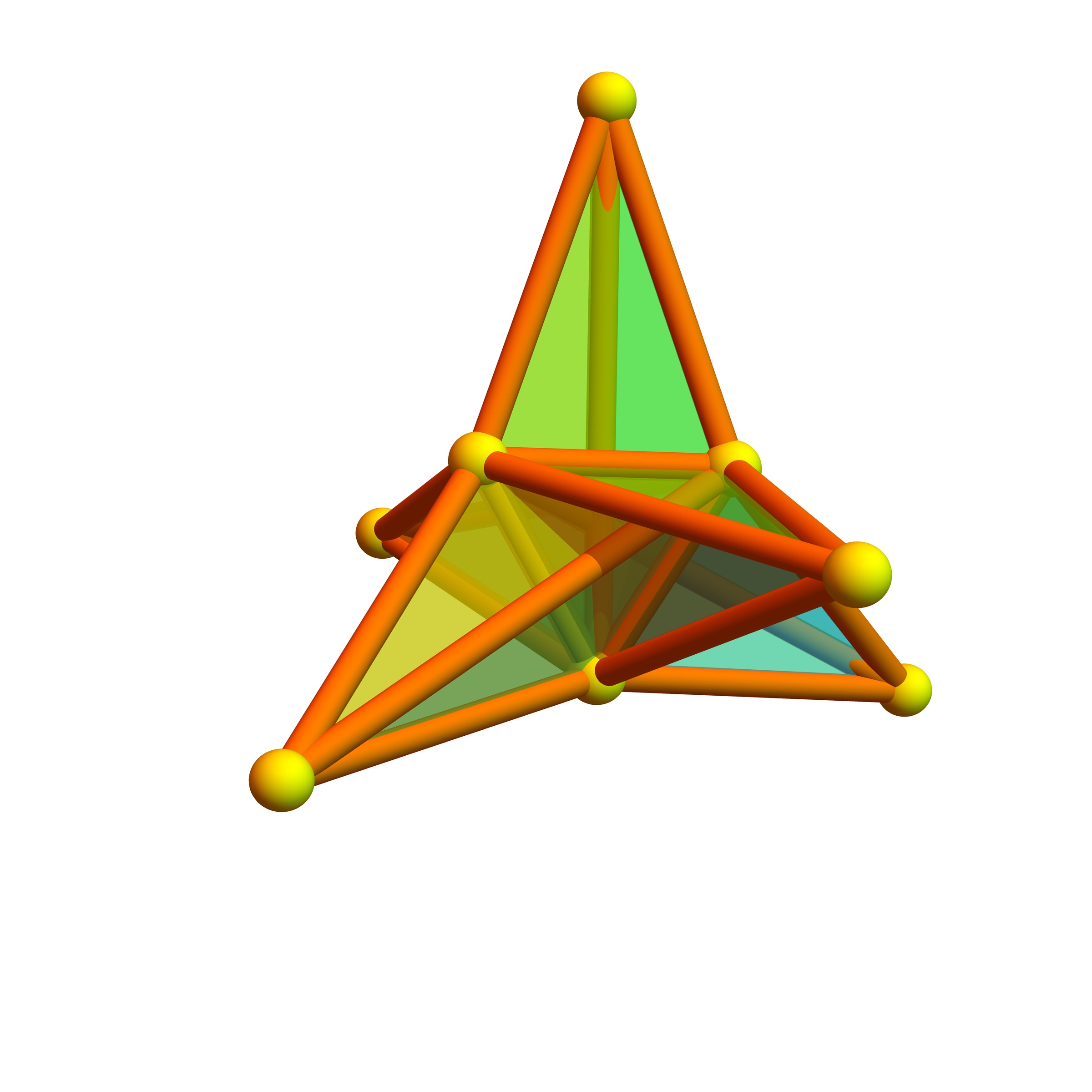
An interesting case is when the target complex is $P=K_{(2,2,2,2)}$ which is a 3-sphere, the 3-dimensional cross polytop, one of the regular polytops in ambient dimension $4$. We can implement the quaternion group $Q$ on $P$, as we can identify the $8$ points in $P$ with $1,-1,i,-i,j,-j,k,-k$. In other words, a map $f$ from $G$ to the quaternion group $Q$ which not have an Abelian image, produces a co-dimension $3$ manifold $H(G,f,P)$, where $P$ is the 3-sphere simplicial complex structure on $Q$ coming from the partition $p=(2,2,2,2)$. In particular, any map from a 4-manifold to $Q$ with this property produces a co-dimension $3$ manifold $H(G,f,P)$ which must be a finite collection of 1-dimensional cycle graphs.

The empty case is rare. For the smallest 3-sphere $G=K_{(2,2,2,2)}$ and the triangle $P=K_{(1,1,1)}$, there are $5796$ surjective maps. There are only 24 cases, where $H$ is empty. They are the maps to $\{1,2,3\}$ where only one number appears more than once.

If $P$ is a $k$-dimensional partition complex and $y$ is a facet in $P$ which is in the image of $f$, then $f^{-1}(y)$ is a $(d-k)$-manifold with boundary or empty. This allows us to construct without much effort manifolds with boundary or pictures of cobordism examples: if the boundary of the manifold is split into two sets $A,B$, then $A,B$ are by definition cobordant. In illustrations done before, like for the expository article [5] in 2012, we needed to construct by hand the ”hose manifold”. We later would use triangulations which numerical methods would provide when parametrizing surfaces $\vec{r}(u,v)$ where $(u,v)\subset\mathbb{R}^{2}$ is a closed region in the parameter plane. The code provided in the code section is shorter than what one needs to get in order to rely on numerical schemes used by computer algebra systems for drawing surfaces. The code works for manifolds of arbitrary dimension.

The semi-ring of partition complexes $\mathcal{P}$ contains the semi-ring of integers and is contained in the Sabidussi ring $\mathcal{G}$ of all graphs, where the addition is the Zykov join [14] and the multiplication is the large multiplication [11]. See [3] for graph multiplications. The semi-ring is dual to the Shannon semi-ring, where the addition is the disjoint union and the multiplication is the strong product [13]. Each of the rings can be augmented to rings by group completing the additive monoid structure. In the Zykov-Sabidussi picture, the “integers” $\mathbb{Z}$ are given by complete graphs $K_{n}$. Because the join $K_{n}\oplus K_{m}=K_{n+m}$ and the large multiplication $K_{n}\otimes K_{m}=K_{nm}$ the map $n\to K_{n}$ is an isomorphism of $\mathbb{Z}$ to $\mathcal{Z}$. When written as partition, $K_{n}=K_{(1,1,\dots,1)}$. The complex $K_{(n)}$ is classically denoted with $\overline{K_{n}}$.

For partitions, $n=(n_{0},\dots,n_{k})$, $m=(m_{0},\dots,m_{l})$, the addition is the concatenation $n+m=(n_{0},\dots,n_{k},m_{0},\dots,m_{l})$. Multiplication is product $n*m=(n_{0}m_{0},n_{1},m_{0},\dots,n_{k}m_{0},n_{1}m_{0}$, $\dots$, $n_{1}m_{l},\dots,n_{k}m_{0}\dots,n_{k}m_{l})$. It obviously enhances the standard multiplication in the case $0$-dimensional case $k=0,l=0$. The order in a partition does not matter. The partition $(2,3)$ is the same than the partition $(3,2)$. For example $(3,4)+(2,1)=(3,4,2,1)$ and $(3,4)*(2,1,1)=(3,3,4,4,6,8)$ or $(1,1,1)*(2,3,4)=(2,2,2,3,3,3,4,4,4)$. Also partitions form so a semi-ring $(P,+,*,0,1)$, and can be enhanced to be a ring. The dimension of a partition $n$ is the number of elements minus $1$. Giving a partition on $[1,n]=\{1,\dots,n\}$ into $k+1$ sets defines a $k$-dimensional simplicial complex and so a k-dimensional Alexandrov topology on $[1,n]$. The maximal possible dimension $n-1$ is achieved, if we take the partition $(1,1,\dots,1)$ of $n$. In the zero dimensional case $n=(n)$, we have the discrete topology.

Every partition $p:$ $n=(n_{0},\dots,n_{k})$ defines a $(k+1)$-partite graph $K_{p}=K_{(n_{0},\dots,n_{k})}$ defined as the join $\oplus_{j=0}^{k}\overline{K_{n_{j}}}$ of the $0$-dimensional graphs $K_{(n_{j})}=\overline{K_{n_{j}}}$. A partition of dimension $k$ defines a $k$-dimensional graph in the sense that the maximal clique has has size $k+1$. The multiplication of partitions corresponds to the large multiplication of graphs first considered by Sabidussi. Any partition in which one of the elements is prime therefore is a multiplicative prime in this ring. The additive primes in the partition ring are the 0-dimensional partitions $(n)$. They can not be written as a sum of smaller partitions.

The complete $(k+1)$-partite graphs are defined by one of the $p(n,k+1)$ partitions $n_{0},\dots,n_{k}$ of $n$. For $n=7$ for example, there are $p(7)=15$ partitions over all. For $n=4$, there is only one 2-dimensional complex, the case when $p=(1,1,2)$. For $k>0$, the graphs are (k+1)=partite graphs $K_{(n_{0},\dots,n_{k})}$. For $k=0$, we have $K_{(n)}=\overline{K_{n}}$ which is the zero-dimensional graph with n-vertices. ¹¹1Mathematica identifies $CompleteGraph[\{5\}]$ with $CompleteGraph[\{1,1,1,1,1\}]$ which is inconsistent with the picture that it should be the join of $k$ graphs $K_{1}$. Of course, one should keep the notation $CompleteGraph[5]$ as $K_{5}$ as it is entrenched. We use $GraphComplement[CompleteGraph[{5}]]$ to get the $0$-dimensional $K_{(5)}$.

The theory of partitions is rich. Euler already noticed that taking products of geometric series produces the generating function for partitions $\sum_{n}p(n)x^{n}=\prod_{k}(1-x^{k})^{-1}$. The fact that partitions naturally define a ring, extending the ring of integers, appears to be less known. To see a partition as a choice of topology on $[1,n]$ even less. We actually consider a partition $p$ as a partition complex $P$ on $[1,n]$ and so as a topological structure of dimension $k$ on the “point” $[1,n]$. A map $f:G\to P$ is regular, if the image is $k$ dimensional. This notion replaces the maximal rank condition of the Jacobian matrix $df$ of a smooth map $f$. An other picture is to see $P$ as a “particle” as Wigner proposed in 1939 already to see irreducible representations of groups as particles.

Lets look at some figures. The first figures shows the case of a $5$ manifold $G=I\oplus I$, with icosahedron 2-sphere $I$ to $P=K_{(1,1,1,1)}$. We took then a random map from the vertex set $\{1,\dots,24\}$ to $\{1,2,3,4\}$ like $(3,4,1,2,2,3,4,2,2,2,2,1,4,4,4,2,1,4,3,1,3,4,4,4)$ for the picture. Each of the 274701298344704 surjective maps from $\{1,\dots,24\}$ to $\{1,2,3,4\}$ produces a 2-manifold. There is no exception.

The additive Zykov monoid $(\mathcal{G},\oplus)$ of graphs contains various interesting sub-monoids. One of them is the monoid $(\mathcal{S},\oplus)$ of spheres. If $A$ is a $k$-sphere and $B$ is a $l$-sphere, then $A+B$ is a $k+l+1$ sphere as indicated already in the introduction. Manifolds are finite simple graphs for which all unit spheres $S(x)$ are in $\mathcal{S}$. Manifolds however are not a sub-monoid and spheres do not form a subring. The Dehn-Sommerville monoid $\mathcal{D}$ is interesting as it generalizes spheres. See [7]. The class $\mathcal{D}$ is inductively defined as a graph $G$ for which all unit spheres are in $\mathcal{D}$ of dimension $1$ less and such that $\chi(G)=1+(-1)^{d}$, where $d$ is the dimension starting with the assumption that the empty graph $0$ in $\mathcal{D}$ of dimension $-1$. Also the Dehn-Sommerville class is not invariant under multiplication. Interesting about Dehn-Sommerville is that unlike spheres, that the definition does not invoke homotopy notions.

We now look at a geometric characterization of the partition monoid $(\mathcal{P},\oplus)$. Let $\mathcal{Q}$ be the set of graphs which have the property that it contains $0$ and such that it is closed under taking unit spheres: all $S(x)$ are in $\mathcal{Q}$ of one dimension less. The Partition monoid actually agrees with this elegant definition:

The class $\mathcal{P}$ of partition graphs has a nice recursive definition. The graphs $\mathcal{P}$ are also characterized number theoretically in that all additive primes in the monoid are zero-dimensional. In the dual Shannon picture, $\hat{\mathcal{P}}$ consists of disjoint union of complete graphs. If one of the additive factors is $1$, it is contractible, meaning that there exists a vertex (actually one can take any vertex), such that $G\setminus\{x\}$ is contractible. The cohomology in general however is not trivial. For the utility graph $K_{(3,3)}$ for example, the Betti vector is $(1,4)$. In general, the Betti vector of $G\in\mathcal{P}$ is $(1,0,\dots,\prod_{j=0}^{k}(n_{j}-1))$ for $k>0$ and $n_{0}$ for $k=0$. In particular, for cross polytopes $p=(2,2,\dots,2)$, it is $(1,0,\dots,1)$. The inductive dimension of $G\in\mathcal{P}$ is defined as the average of the dimensions of the unit spheres is equal the maximal dimension. They are small graphs of diameter $1$ or $2$ and have the property that given any finite set of points, then the intersection of all these unit spheres is again in the class. We should think of elements in $\mathcal{P}$ of dimension $k$ therefore as generalized $k$-dimensional points. Complete graphs $K_{k+1}=K_{(1,\dots,1)}$ are just a special case. The intersection of $\mathcal{P}$ and spheres $\mathcal{S}$ is the set of cross polytopes, where every additive prime factor is a zero-dimensional sphere $K_{(2)}=\overline{K_{2}}$. In short, elements in $\mathcal{P}$ can serve as $k$-dimensional points.

Some Mathematica code appeared already in [8], where we considered the case of maps $f:G\to\mathbb{R}^{k}$. The abstract version is much more elegant because we do not have to program each dimension separately. It can serve also as pseudo code.

By the way, the addition in the monoid of partitions is already called Join $Join[\{1,2,3\},\{1,6,6\}]$ gives $\{1,2,3,1,6,6\}$. This fits, as the graph $K_{(1,2,3,1,6,6)}$ is the Zykov join of $K_{(1,2,3)}$ and $K_{(1,6,6)}$. The Zykov join is in the Wolfram language known as GraphJoin.

The following code generates all surjective maps and analyzes in each case the topology. This works only for very small host manifolds. To see the topological nature of the manifolds, we look at the cohomology in the form of Betti vectors $(b_{0},b_{1},\dots b_{d})$ which gives the dimensions $b_{k}$ of the harmonic $k$-forms of the complex. This in particular gives the number of connectivity components $b_{0}$ or the genus $b_{1}/2$, which is for surfaces the “number of holes”.

Example 1: In the list of all co-dimension 2 curves in the smallest 3 sphere $K_{(2,2,2,2)}$. There were 4848 single circles,888 cases with 2 circles and 36 cases with 4 circles. There were 5772 surjective maps from $G$ to $K_{3}$ which produced a non-empty surfaces. For only 24 cases, the resulting manifold is empty.

Example 2: Take the smallest 4 sphere $K_{(2,2,2,2,2)}$. There were 55980 surjective maps from $G$ to $K_{3}$. This produces co-dimension 2 surfaces. Only 30 surjective function sproduced an empty surface. The other 55950 produced either 2-spheres (50160), 2 disjoint 2-spheres (3960) or 4 disjoint 2-spheres (60 cases) or single $2$-tori (1680 cases) or 2 disjoint $2$-tori (90 cases).

Example 3: For all co-dimension $1$ surfaces in the 4-sphere $G=K_{(2,2,2,2,2)}$, we see $992$ 3-spheres, $20$ cylinders $S^{2}\times S^{1}$ and $10$ pairs of disjoint sphere. There were $1022$ surjective maps from $G$ to $K_{2}$, so that 30 produced empty sets.

Example 4: All co-dimension 1 surfaces in a small projective 3-manifold $\mathbb{RP}^{3}$ produce $2046=2^{12}-2$ possible surjective maps to $K_{2}$. All of them give surfaces. There are $548$ spheres, $1394$ tori, $68$ genus 2 surfaces, $8$ genus 3 surfaces, $20$ pairs of spheres, $8$ pairs with one sphere and one torus and 2 pairs, where one is a $2$-torus and one a genus 2 surface.

Example 5: When looking at co-dimension 2 surfaces in a small implementation of the 4-manifold $\mathbb{CP}^{2}$, we count $8748$ 2-spheres and $9402$ tori.

Example 6: Among all co-dimension 1 surfaces in a small implementation of $\mathbb{CP}^{2}$ we count $511$ 3-spheres.

Example 7 For all hyper-surfaces defined by $K_{2}$ in the small 4-manifold $\mathbb{S}^{2}\times\mathbb{S}^{2}$ defined by surjective to $K_{2}$ the nuumber of $3$-manifolds is 2046. There were 1446 3-spheres with Betti vector $(1,0,0,1)$ and 600 generalized tori $S^{2}\times S^{1}$ with Betti vector $(1,1,1,1)$.

Example 8 looks for co-dimension 2 surfaces in a small $G=S^{2}\times S^{2}$ using the triangle $P=K_{3}$. There are $42288$ two-spheres, $71022$ genus 1 surfaces ($2$-tori), $48210$ genus 2 surfaces, $7788$ genus 3 surfaces, $660$ genus 4 surfaces, $78$ genus 5 surfaces and 960 disconnected pairs of 2-spheres. In total, the cohomology of $171006$ surfaces was computed.

Example 9 For all hyper-surfaces in the small 3 sphere $K_{(2,2,2,2)}$ with $P=K_{(1,2)}$ we have $5496$ surfaces, where $5456$ were 2-spheres, $84$ were $2$-tori and $256$ were double spheres.

Example 10 For all hyper-surfaces in the small 3 sphere $G=K_{(2,2,2,2)}$ with $P=K_{(1,3)}$ we have $40824$ cases in total, no empty surfaces, $38448$ spheres, $216$ tori and $2160$ double spheres. In this case we look at all maps from $G$ to $\{1,2,3,4\}$ because $P$ has $4$ vertices. This requires to look at much more maps. An interesting question is how large the total number of hyper-surfaces $\bigcup_{P}\bigcup_{f}H(G,f,P)$ can become. As they are all sub-graphs of the Barycentric refinement $G_{1}$ of $G$, there are only finitely many. Many $H(G,f,P)$ are are actually the same graph.

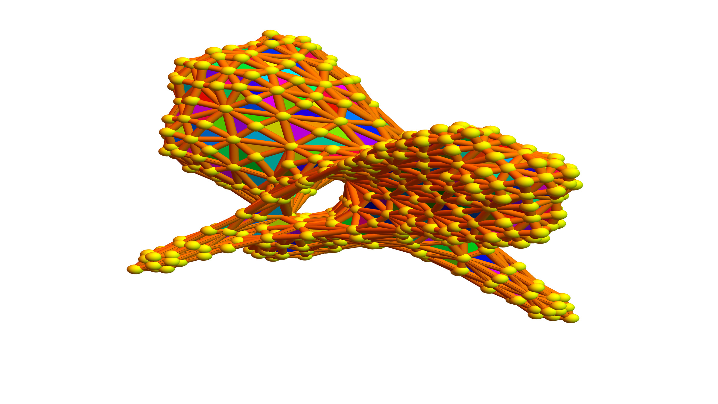
As the gallery in the next section illustrates, much more interesting sub-manifolds are possible for larger host manifolds $G$. But the number of possible maps is too large for an exhaustive list. We would have to use Monte-Carlo simulations to investigate what manifolds typically occur.

References

- [1] P. Alexandroff. Diskrete Räume. Mat. Sb. 2, 2, 1937.
- [2] G. Cuisenaire and C. Gattegno. Numbers in Colour: A New Method of Teaching the Processes of Arithmetic to All Levels of the Primary School. Heinemann, 1957.
- [3] R. Hammack, W. Imrich, and S. Klavžar. Handbook of product graphs. Discrete Mathematics and its Applications (Boca Raton). CRC Press, Boca Raton, FL, second edition, 2011. With a foreword by Peter Winkler.
- [4] O. Knill. Anschauliche additive Zahlentheorie. In B. Roethlin, editor, Schweizer Jugend forscht year book 83., pages 200–210. Winterthur: Verlag Schweizer Jugend forscht, 1983.
- [5] O. Knill. The theorems of Green-Stokes,Gauss-Bonnet and Poincare-Hopf in Graph Theory. http://arxiv.org/abs/1201.6049, 2012.
-
[6]
O. Knill.
A Sard theorem for graph theory.
http://arxiv.org/abs/1508.05657, 2015. -
[7]
Dehn-Sommerville from Gauss-Bonnet.
https://arxiv.org/abs/1905.04831, 2019. - [8] O. Knill. Cohomology of Open sets. https://arxiv.org/abs/2305.12613, 2023.
- [9] O. Knill. Finite topologies for finite geometries. https://arxiv.org/abs/2301.03156, 2023.
- [10] A.P. Morse. The behavior of a function on its critical set. Ann. of Math. (2), 40(1):62–70, 1939.
- [11] G. Sabidussi. Graph multiplication. Math. Z., 72:446–457, 1959/1960.
- [12] A. Sard. The measure of the critical values of differentiable maps. Bull. Amer. Math. Soc., 48:883–890, 1942.
- [13] C. Shannon. The zero error capacity of a noisy channel. IRE Transactions on Information Theory, 2:8–19, 1956.
- [14] A.A. Zykov. On some properties of linear complexes. (russian). Mat. Sbornik N.S., 24(66):163–188, 1949.