Making Bias Amplification in Balanced Datasets Directional and Interpretable

To measure the leakage of an attribute ($A$) from a task ($T$), Wang et al. [11] trained an attacker function ($f$) that takes $T$ as input to predict $A$. The performance of the attacker is measured using a quality function ($Q$). Previous works [11, 3] used accuracy and F1-scores for $Q$. Wang et al. [11] describe dataset leakage ($\lambda_{D}$) as:

where $T$ and $\hat{T}$ represent the ground truth and model predictions for the task, respectively. $f_{D}$ is trained on task observations from the dataset, while $f_{M}$ is trained on task predictions from the model.

Leakage amplification measures the increase of leakage in model predictions compared to the leakage in the dataset:

Model predictions ($\hat{T}$) are not $100\%$ accurate and might have errors. These errors might create a difference in leakage values, which could be misinterpreted as bias. To prevent conflation of errors with bias, Wang et al. [11] introduced a similar error rate in $T$ using random perturbations. If the model predictions $\hat{T}$ are $70\%$ accurate, they randomly flipped $30\%$ of labels in $T$. As the bias in $T$ can vary significantly between two random perturbations, they measured bias amplification using confidence intervals. This quality equalization prevents conflation of model biases and errors.

As noted in section 3.2.1, Wang et al’s [11] formula for leakage amplification is not compatible with directionality as it has fixed posteriors, not priors. We define predictability ($\Psi$) using fixed priors.

$f^{A}$ represents an attacker function that takes $T$ as input and tries to predict $A$. $f^{T}$ represents an attacker function that takes $A$ as input and tries to predict $T$.

While leakage amplification computed the difference between $\lambda_{M}$ and $\lambda_{D}$, we normalize the difference in predictability using their sum.

COMPAS [1] is a dataset containing information about individuals who have been previously arrested. Each entry is associated with 52 features. We used five features: age, juv_fel_count, juv_misd_count, juv_other_count, priors_count.

We limited the dataset to 2 races (Caucasian or African-American) which we used as the protected attribute ($A$). The task ($T$) was recidivism (i.e. if the person was arrested again for a crime in the next 2 years). Hence, $A=\{\texttt{Caucasian}:0,\texttt{African-American}:1\}$ and $T=\{\texttt{No Recidivism}:0,\texttt{Recidivism}:1\}$.

We created balanced and unbalanced versions of the COMPAS dataset. For the unbalanced dataset, we sampled all available COMPAS instances (attributes, race labels, and recidivism labels) for each of the four $A$ and $T$ pairs. For the balanced dataset, we sampled an equal number of instances across the four $A$ and $T$ pairs. The counts for the $A$ and $T$ pairs in the unbalanced dataset are shown in the top-left quadrant of Table 2(a), while the counts for the balanced dataset are shown in the top-right quadrant of Table 2(b).

We trained a decision tree model on the unbalanced and the balanced COMPAS datasets. Each model predicts a person’s race ($A$) and recidivism ($T$) based on the $5$ selected features. We measured the bias amplification caused by each model in two directions: bias amplification caused by race ($A$) on recidivism ($T$), referred to as $A\rightarrow T$, and the bias amplification caused by recidivism ($T$) on race ($A$), referred to as $T\rightarrow A$. We compared our proposed metric, $DPA$, to previous metrics $BA_{\rightarrow}$ and $Multi_{\rightarrow}$. For $DPA$, we used a 3-layer dense neural network (with a hidden layer of size 4 and sigmoid activations) as the attacker model for both directions. Following [11], we evaluated each bias amplification metric on the training set predictions.

Next, we explore how different bias amplification metrics are impacted in $T\rightarrow A$ as a model’s reliance on task-associated objects to predict gender increases. We used the gender-annotated version of the COCO dataset released by Wang et al. [11]. Each image is labeled with both gender ($\texttt{A}=\{\texttt{Female}:0,\texttt{Male}:1\}$) and object categories ($\texttt{T}=\{\texttt{Teddy Bear}:0,\ldots,\texttt{Skateboard}:78)\}$. For the purpose of the experiment, we sampled 2 sub-datasets, “Unbalanced” and “Balanced”. The balanced dataset is subject to the following constraint.

We used the same 12 objects for the unbalanced case but relaxed the constraint from Equation 15 as shown in equation 16. This results in a dataset of 15743 images (8885 male and 6588 female images)

For each dataset, we have 4 versions: one original and three perturbed versions wherein the person in the image is masked using different techniques (i.e., partially masking segment, completely masking segment, completely masking bounding box), as shown in Table 4. We trained a separate VGG16 [9] (pre-trained on ImageNet-1K [7]) for 12 epochs for each of the 8 cases (4 versions for both balanced and unbalanced datasets). We measure the feature attribution of the model using Gradient-Shap [6]. This allows us to measure the attribution of different image elements and compare it with $T\rightarrow A$ bias amplification reported by various metrics.

In Table 4, the “attribution score” is a measure of the contribution of non-person image elements in the model’s prediction of a person’s gender. To calculate the attribution score, we take the normalized attribution map created using Gradient-Shap [6] and mask the values for the person’s segment (similar to the segment-masked case). We add the remaining values and average across all images in the dataset to get the final score.

The unbalanced section in Table 4 shows that all metrics report increasing scores as the attribution score increases. It makes intuitive sense that as the model relies more on the background objects (including task-associated objects) to predict gender, the bias of tasks on gender (i.e., $T\rightarrow A$) increases.

But, in Table 4’s balanced section, this trend no longer holds for $BA_{\rightarrow}$. $BA_{\rightarrow}$ reports a constant zero bias amplification despite the model’s increasing reliance on background objects to predict gender. Thus, for balanced datasets, $BA_{\rightarrow}$ continues to report zero bias amplification despite changes in model biases.

Thus, $DPA$ is the most reliable metric as it avoids pitfalls such as $BA_{\rightarrow}$’s inability to work with “balanced” datasets and $Multi_{\rightarrow}$’s inability to distinguish positive and negative bias amplification.

As we observed in Section 6, each metric reported a different value for bias amplification. This makes it challenging for users to decide which metric to use when measuring bias amplification.

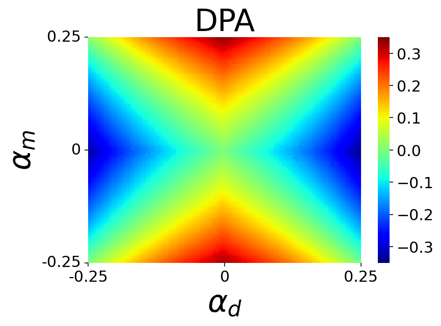
To understand the behavior of each metric, we simulated the following scenario. Consider a dataset with a protected attribute $A$ (where $A=0$ or $A=1$) and task $T$ (where $T=0$ or $T=1$). Initially, we have the same probability ($0.25$) for each $A,T$ pair. To introduce bias in the dataset, we modify the probabilities for specific groups. We add a term $\alpha$ to the group {$A=0$, $T=0$} and subtract it from {$A=1$, $T=1$}. Here, $\alpha$ ranges from $-0.25$ to $0.25$ in steps of $0.005$. This setup creates a dataset that is balanced only when $\alpha=0$; as $\alpha$ moves away from $0$ (in either direction), the dataset becomes increasingly unbalanced. We follow the same setup to simulate the model predictions.

With $\alpha$ ranging from $-0.25$ to $0.25$, we create $100$ different versions of the dataset and model predictions, influenced by $\alpha_{d}$ and $\alpha_{m}$, respectively. For each metric, we plot a $100\times 100$ heatmap of the reported bias amplification scores. Each pixel in the heatmap represents the bias amplification score for a specific {dataset, model} pair.

Figure 2 shows the heatmaps for all metrics. Figures 2(a) and 2(b) display the bias amplification heatmaps for $BA_{\rightarrow}$ and $DPA$, respectively. These heatmaps look similar, suggesting that both metrics show similar behavior. However, $BA_{\rightarrow}$ (Figure 2(a)) shows a distinct vertical green line in the center, indicating that when the dataset is balanced ($\alpha_{d}=0$ on the X-axis), bias amplification remains at $0$, regardless of changes in model’s bias (indicated by varying $\alpha_{m}$ values on the Y-axis). In contrast, $DPA$ (Figure 2(b)) accurately detects non-zero bias amplification whenever there is a shift in bias in either the dataset or model predictions. Thus, $DPA$ is a more reliable metric for measuring bias amplification. $Multi_{\rightarrow}$ (as shown in Figure 2(c)) reports positive bias amplification in all scenarios, making it an unreliable metric.

While $DPA$ is generally the most reliable metric for measuring bias amplification, there are cases where $BA_{\rightarrow}$ is more suitable. Consider a job hiring dataset: $100$ men ($A=0$) and $50$ women ($A=1$) apply for a job. Out of these, $25$ men and $25$ women are hired ($T=0$), while the rest are rejected ($T=1$). Since the acceptance rate for women ($50\%$) is higher than for men ($25\%$), $BA_{\rightarrow}$ sees this as a bias. In contrast, $DPA$ interprets this as an unbiased scenario because the same number of men and women are hired. In situations like this, where $T=0$ (acceptance) is almost always less frequent than $T=1$ (rejections), $BA_{\rightarrow}$ may be a better fit, as it considers a dataset unbiased only if the $T=0$-to-$T=1$ ratio is the same for both genders.

In another scenario, imagine a dataset of men ($A=0$) and women ($A=1$), where each person is either indoors ($T=0$) or outdoors ($T=1$). It would make more sense to call this dataset unbiased when there are an equal number of instances for all $A$ and $T$ pairs. In this case, $DPA$ is a better metric, as it treats a dataset as unbiased when all $A$ and $T$ combinations have equal representation. $BA_{\rightarrow}$ and $DPA$ each measure distinct types of bias. The choice of metric depends on the specific bias we aim to address.

References

- Angwin et al. [2022] Julia Angwin, Jeff Larson, Surya Mattu, and Lauren Kirchner. Machine bias. In Ethics of Data and Analytics, pages 254–264. Auerbach Publications, 2022.
- Foulds et al. [2020] James R. Foulds, Rashidul Islam, Kamrun Naher Keya, and Shimei Pan. An intersectional definition of fairness. In 2020 IEEE 36th International Conference on Data Engineering (ICDE), pages 1918–1921, 2020.
- Hirota et al. [2022] Yusuke Hirota, Yuta Nakashima, and Noa Garcia. Quantifying societal bias amplification in image captioning. In Proceedings of the IEEE/CVF Conference on Computer Vision and Pattern Recognition, pages 13450–13459, 2022.
- Lin et al. [2019] Kun Lin, Nasim Sonboli, Bamshad Mobasher, and Robin Burke. Crank up the volume: preference bias amplification in collaborative recommendation, 2019.
- Lin et al. [2014] Tsung-Yi Lin, Michael Maire, Serge Belongie, James Hays, Pietro Perona, Deva Ramanan, Piotr Dollár, and C Lawrence Zitnick. Microsoft coco: Common objects in context. In Computer Vision–ECCV 2014: 13th European Conference, Zurich, Switzerland, September 6-12, 2014, Proceedings, Part V 13, pages 740–755. Springer, 2014.
- Lundberg and Lee [2017] Scott M Lundberg and Su-In Lee. A unified approach to interpreting model predictions. In Advances in Neural Information Processing Systems. Curran Associates, Inc., 2017.
- Russakovsky et al. [2015] Olga Russakovsky, Jia Deng, Hao Su, Jonathan Krause, Sanjeev Satheesh, Sean Ma, Zhiheng Huang, Andrej Karpathy, Aditya Khosla, Michael Bernstein, Alexander C. Berg, and Li Fei-Fei. ImageNet Large Scale Visual Recognition Challenge. International Journal of Computer Vision (IJCV), 115(3):211–252, 2015.
- Seshadri et al. [2023] Preethi Seshadri, Sameer Singh, and Yanai Elazar. The bias amplification paradox in text-to-image generation. arXiv preprint arXiv:2308.00755, 2023.
- Simonyan and Zisserman [2015] Karen Simonyan and Andrew Zisserman. Very deep convolutional networks for large-scale image recognition, 2015.
- Wang and Russakovsky [2021] Angelina Wang and Olga Russakovsky. Directional bias amplification. In International Conference on Machine Learning, pages 10882–10893. PMLR, 2021.
- Wang et al. [2019] Tianlu Wang, Jieyu Zhao, Mark Yatskar, Kai-Wei Chang, and Vicente Ordonez. Balanced datasets are not enough: Estimating and mitigating gender bias in deep image representations. In Proceedings of the IEEE/CVF International Conference on Computer Vision, pages 5310–5319, 2019.
- Yatskar et al. [2016] Mark Yatskar, Luke Zettlemoyer, and Ali Farhadi. Situation recognition: Visual semantic role labeling for image understanding. In Proceedings of the IEEE conference on computer vision and pattern recognition, pages 5534–5542, 2016.
- Zhao et al. [2023] Dora Zhao, Jerone Andrews, and Alice Xiang. Men also do laundry: Multi-attribute bias amplification. In Proceedings of the 40th International Conference on Machine Learning, pages 42000–42017. PMLR, 2023.
- Zhao et al. [2017] Jieyu Zhao, Tianlu Wang, Mark Yatskar, Vicente Ordonez, and Kai-Wei Chang. Men also like shopping: Reducing gender bias amplification using corpus-level constraints. arXiv preprint arXiv:1707.09457, 2017.
Supplementary Material
Appendix A explanation
To understand why cannot differentiate between positive bias amplification and negative bias amplification (i.e.) bias reduction, let us take a look at its formulation.