A theory of Stimulated and Spontaneous Axion Scattering
Abstract
We present a theory for nonlinear, resonant excitation of dynamical axions by counter-propagating electromagnetic waves in materials that break both and symmetries. We show that dynamical axions can mediate an exponential growth in the amplitude of the lower frequency (Stokes) beam. We also discuss spontaneous generation of a counter-propagating Stokes mode, enabled by resonant amplification of quantum and thermal fluctuations in the presence of a single pump laser. Remarkably, the amplification can be orders of magnitude larger than that obtained via stimulated Brillouin and Raman scattering processes, and can be modulated with the application of external magnetic fields, making stimulated axion scattering promising for optoelectronics applications.
Introduction.—
The propagation of electromagnetic (EM) fields through materials is governed by the celebrated Maxwell’s equations. In vacuum, these equations arise from the usual electromagnetic action , where and are the electric and magnetic fields and and are the vacuum permittivity and permeability, respectively. For waves in a medium, it often suffices to promote these constants to material dependent values without changing the form of the action. However, in materials that break time reversal () and inversion () symmetries, a novel term becomes possible
| (1) |
with a pseudoscalar field (odd under both and ) coupled to electromangetic fields with strength . This unusual term first appeared in quantum chromodynamics in the context of the strong charge conjugation-parity problem [1, 2, 3]. The elementary excitations of the field, “axions”, are one of the prime candidates for cosmological dark matter [4]. Despite significant efforts [5, 6, 7, 8, 9, 10, 11, 12, 13], they are yet to be detected experimentally.
The magnetoelectric coupling (1) has been known to exist in materials like Cr2O3 for quite some time [14, 15, 16]. The corresponding action, , typically requires breaking both and symmetries. However, recently it has been recognized that even in the presence of and/or , such a coupling can exist, if is given by , with the speed of light, the fine structure constant, and is an integer multiple of . Having with odd is the defining characteristic of topological insulators and is the origin of the topological magnetoelectric effect [17, 4, 2, 20].
When both and symmetries are broken, is no longer quantized. This is the case in Cr2O3, but also some magnetically doped topological insulators [2, 6]. In the latter, finite antiferromagnetic (Neel) order leads to the deviation of from , and longitudinal fluctuations of the Neel order parameter translate into fluctuations of . To avoid confusion with the static part of , these fluctuations are sometimes referred to as dynamical axions (DAs). DAs can hybridize with photons, forming axion-polaritons, and can manifest in a variety of dynamical responses [3, 23, 24, 25, 26, 27]. Recent experimental work in thin film MnBi2Te4, which is predicted to host DAs, not only observed an axion-like coupling between the Neel order and [28] but also directly probed DAs [29].
In this Letter, we focus on an inherently nonlinear phenomenon associated with light propagation in media supporting DAs, namely stimulated axion scattering (SAS). We show that the nonlinear excitation of DAs by two counterpropagating and orthogonally polarized fields leads to energy transfer between the two waves, with the intensity of the lower frequency (Stokes) mode growing exponentially in space. This can lead to reflection and transmission coefficients of the Stokes mode to be greater than , and provides a sensitive probe of axion dynamics in the material. We also show that the Stokes mode can be generated spontaneously in the presence of a single applied electromagnetic wave when allowing for quantum or thermal fluctuations of the Neel order. Apart from providing a method for axion spectroscopy, this latter phenomenon can be employed to realize the phase conjugation effect [30], which can be used in holography and image correction [31].
The exponential growth of the Stokes mode in SAS is similar to that seen in Stimulated Brillouin Scattering (SBS) [32] and Stimulated Raman Scattering (SRS) [33]. Instead of axions, the oscillator modes that enable SBS and SRS are atomic or molecular vibrations. Due to their high sensitivity, SBS and SRS have found applications in microscopy and spectroscopy both in inroganic materials and biological systems [34, 35, 36, 37, 38]. Furthermore, the orthogonality of polarizations which maximizes SAS, concomitantly minimizes SBS and SRS; this sensitivity to the polarization can thus help isolate these different phenomena. Remarkably, even though the DA is driven by the product of the electric and magnetic fields, which one naively would expect to have weaker coupling to matter than the product of electric fields, the exponential amplification rate for SAS can be orders of magnitude larger than for SBS and SRS. This difference arises from the relatively low stiffness of the DA as compared to phonons, making DAs easier to excite. The strength of SAS and its tunability with external fields point towards possible practical importance of materials that host DAs for various optoelectronics applications where SBS and SRS are currently employed [39, 40].
Equations of Motion.— The minimal action for the coupled EM fields and DAs in a material is given by
| (2) |
Here we allow the permeability and permittivity to deviate from their vacuum values. is the coupling between the EM fields and the DA, and are the stiffness, velocity, and mass of the DA, respectively. For the remainder of this letter, we neglect the static part of , as it only weakly affects SAS (see discussion in SI).
Minimizing the action leads to the coupled equations of motion
| (3a) | ||||
| (3b) | ||||
Here is the speed of light in the material and the current due to DAs is given by , where the polarization and magnetization induced by the DA are and , respectively. A rate has been introduced phenomenologically to describe the damping of axions (which in turn relates to the relaxation of appropriate spin waves in the material).
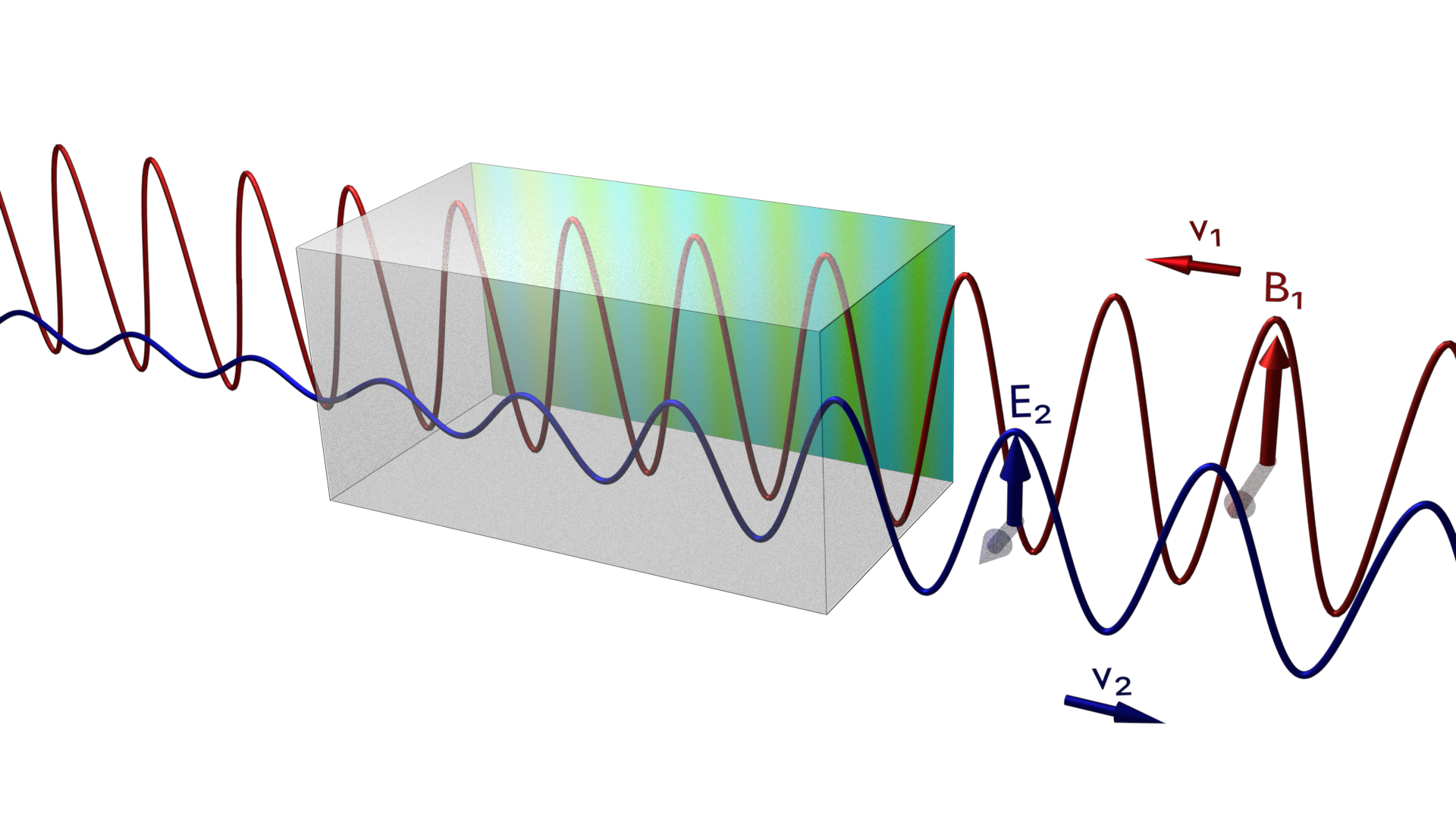
As depicted in Fig. 1, we consider two counter propagating electromagnetic waves, + c.c., where are the slowly varying envelope functions and and their frequency and wavevector in the DA medium, respectively; the waves are oriented such that and propagating along the -axis. In the following we will ignore the spatial derivative part on the LHS of (3b), using the fact that the axion velocity is much smaller than the speed of light. Then, if the difference of the incoming light beam frequencies matches the DA energy , DAs will be resonantly excited. We refer to the higher frequency () mode as the pump, and the lower frequency () mode as the Stokes mode. We will also assume that , which allows us to use the rotating wave approximation. Making the ansatz + c.c., with and plugging in the solution for from Eq. (3b) into Eq. (3a), we find for the envelope functions in the slowly varying envelope approximation:
| (4a) | ||||
| (4b) | ||||
In the limit when can be assumed constant (), the RHS of Eq. (4b) can be viewed as giving an imaginary contribution to the index of refraction, which on resonance, , goes as , where is the gain coefficient defined below in Eq. (6) and is the intensity of the pump. This imaginary contribution to the index of refraction makes the amplitude of the Stokes mode grow exponentially as a function of .
We can find time-independent solutions to the above equations for arbitrary incoming beam intensities and frequencies. Writing Eqs. (4) in terms of the intensites , their real parts yield
| (5a) | ||||
| (5b) | ||||
where
| (6) |
Here, is the gain coefficient for the SAS process mentioned above, and is the index of refraction of the DA medium. Note that Eqs. (5) imply which can be interpreted as the conservation of photon number between the Stokes and pump fields (single absorbed pump photon converts into single Stokes photon and DA). The pump beam enters the sample at , while the Stokes beam at the opposite end at . In the limit , the output Stokes intensity is readily obtained and found to grow exponentially in both the pump intensity and sample length:
| (7) |
The pump intensity can be obtained using the photon conservation equation; a general solution for arbitrary pump and Stokes intensities is given in the SI.
Effect strength estimate. We now estimate using model parameters for Bi2Se3 doped with Fe [4]. The axion stiffness is given by (see SI for more details)
| (8) |
where are parameters in an effective four-band model for the system, are velocities and is the gap at the point. Using eV, such that the band gap is trivial, eVÅ , eVÅ [4], an axion mass meV, magnon lifetime ns, pump frequency THz, index of refraction , and assuming we are on resonance, we find .
Importantly, is proportional to the magnon lifetime and may be larger as magnon lifetimes can exceed ns [1]. Conversely, the gain bandwidth is protortional to the magnon relaxation rate; see Eq. (6). Thus, an increase of the bandwidth can be traded for a decrease in gain amplitude and vice versa. We also note that is inversely proportional to the Neel temperature, as which can be modulated, for instance, by applying a magnetic field perpendicular to the AFM ordering direction. The controllability of gain parameters using external fields makes media supporting DAs potentially more versatile for non-linear amplification than materials where SBS, SRS or inversion breaking non-linearities [42] are employed.
The estimated gain is at least an order of magnitude larger than that obtained with SBS or SRS in materials typically used for nonlinear optics [5]. These processes are similar to SAS with the distinction that SBS and SRS involve lattice and molecular vibrations, respectively, in lieu of axions. The large SAS effect is at first surprising given that SBS and SRS proceed via a putatively stronger coupling , where is a change in the dielectric constant due to lattice or molecular vibrations while the former corresponds to a weaker coupling . In the SI, we argue that the reason for the strength of SAS in comparison to SBS (which in turn is generally stronger than SRS) is because of the lower stiffness of axions compared to phonons, making them easier to excite. Another process used for parameteric amplification when inversion symmetry is absent are non-linearities. Here, the gain coefficient scales as and is generically weaker than that for SAS, SBS, and SRS, but the gain bandwidth is much broader (for a quantiative comparison, see Ref. [42]). In short, SAS is a strong effect that could be used for parameteric amplification depending on the precise requirements of gain, bandwidth, and wavelength of interest.
Finally, we note that the maximum amplification obtainable is not without bounds. The DA amplitude is bounded due to the finite amplitude of the underlying Neel order. The deviation in the static from in AFM topological insulators is given by [3], where is the contribution of the longitudinal AFM order to the electronic parameter introduced above. This limits the amplitude of DA to . Since is excited by the product of the pump and Stokes fields, this puts a bound on the geometric mean of the local intensities, . While this does not bound the relative gain (), it asserts a bound on the maximum output Stokes intensity.
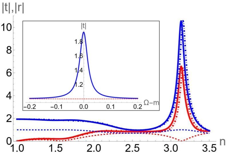
Boundary effects:— We now consider a more detailed treatment of the setup in Fig. 1 accounting for boundary conditions. The bulk equations of motion can be solved semi-analytically and a solution consistent with the boundary conditions can be found numerically by iteration; see SI for details. In Fig. 2, the numerically computed reflectance and transmittance coefficients of the Stokes mode are plotted as a function of index of refraction of the DA medium. We used a sample length m, so that , which simplifies the treatment of the nonlinearity (see SI for details). The electric field amplitudes in the incident waves are V/nm and V/nm; this leads to a gain factor for the Stokes mode at . The transmittance being greater than 1 is a direct consequence of the exponential gain of the Stokes intensity governed by Eq. (7). Moreover, when the index of refraction , reflections at the boundaries occur, and a part of the Stokes beam can exit the sample in the direction opposite to its incidence, resulting in reflectance coefficients that can also exceed one.
Note that the Stokes and pump beam polarizations remain unchanged as they propagate through the medium if has no static part (A static contribution to due to the equilibrium AFM order is generally present; however, even in topological insulators produces only a very small Kerr rotation [25, 16]. See SI for details). This simplification allows one to compute the reflection and transmission coefficients of the Stokes’ mode by geometrically adding up contributions from all possible paths of the beam (with an arbitrary number of internal reflections) accounting for the phase and gain factors accrued along the segments of the path. This analytical computation matches the exact result obtained by numerical iteration well, predicting a series of Fabry-Perot type resonances where the Stokes intensity can be greatly amplified (see an example in Fig. 2, and the analytical derivation in Eqs. (S74-77) of the SI).
Spontaneous Emission:— We now explore the possibility of spontaneous generation of the Stokes mode due to the resonant amplification of quantum or thermal fluctuations in the DA medium in the presence of a single coherent source. Including Langevin fluctuations in Eq. (3b), and solving for and in the presence of a strong and thus approximately spatially constant , we find the average Stokes intensity emitted at (See SI) to be given by [8, 9, 10]
| (9) |
where is the modified Bessel function of the first kind, is the gain factor as defined above, and is an effective seed Stokes intensity,
| (10) |
We assume THz and meV as above, sample cross-section and meV. The temperature and sample cross-section enter due to the average fluctuation strength of the dynamical axion (in the classical limit) as discussed in the SI. In the large gain limit , Eq. (9) shows that the amplitude of the Stokes mode grows exponentially with the length of the sample, much like the stimulated case. We note again that the exponential growth is limited by the condition, , saturating when intensities become comparable.
Conclusion:— SAS described in this paper is a qualitatively strong phenomenon that may be useful for spectroscopic studies of condensed matter axions, and could also have practical applications. For our estimates we considered Bi2Se3 which has well established electronic parameters, and is expected to harbor an AFM phase when doped with Fe (but has not yet been experimentally realized). The band gap and the putative Néel temperature are small—this limits the temperatures where the effect is present, , as well as the frequencies of the electromagnetic sources, . The above discussion also applies to thin films of , which likewise has a small band gap but a relatively large K [28]. Using Eq. (8), we find a similar gain coefficient . We note here that bulk possesses parity symmetry, and thus quantized , which should make SAS vanish in bulk samples. SAS should also be present in known magnetoelectrics, such as . In , a significantly larger band gap (3 eV) allows application of much higher frequency pump and Stokes beams without deleterious bulk absorption, and the high Neel temperature (300 K) [47] should allow for observing SAS at room temperature. The gain coefficient benefits from higher frequency sources, though is likely suppressed by the larger band gap. An accurate estimate of for is left for future work.
We would like to mention that the general framework of stimulated scattering, SAS, SBS, or SRS, thanks to its exquisite selectivity and sensitivity can have many applications in condensed matter systems. In particular, it may be useful for detecting other long sought excitations such as the Higgs mode [48, 49], or dark Josephson plasmons [50].
Finally, it is interesting to consider whether cosmic axions can be excited in a similar fashion by colliding sufficiently strong orthgonally polarized laser beams. The problem of light-by-light scattering has rich history, form the elastic Euler-Heisenberg scattering [51, 52, 53], to inelastic Beit-Wheeler electron-positron pair creation [54]. At low photon frequencies, elastic scattering is extremely weak and hard to detect except in some special cases [55]; inelastic scattering [54], on the other hand, requires very high frequency photons [56]. In this regard, SAS may be advantageous since the axion mass is expected to be in the sub eV range, and axions could be excited resonantly. Even if such experiments do not lead to the detection of cosmic axions, they should put new bounds on the mass and the coupling to this elusive particle.
Note:—
The authors of Ref. [26] considered a similar set up where DAs were excited by counter-propagating electromagnetic waves. They do not include, however, the back-action of DAs on the driving fields crucial in SAS, instead studying the DA contribution to time-resolved Kerr rotations of a probe beam.
Data Availability:—
Acknowledgements:—
We thank V. Quito, P. Orth, S.-Y. Xu, R. McQueeney, J. Curtis, A. Bhattacharya, A. Burkov, A. Hoffman, and D. Basov for useful discussions. This work was supported by the Center for the Advancement of Topological Semimetals (CATS), an Energy Frontier Research Center funded by the U.S. Department of Energy (DOE) Office of Science (SC), Office of Basic Energy Sciences (BES), through the Ames National Laboratory under contract DE-AC02-07CH11358. The work of KA, particularly on the sample boundary effects, was supported by the US Department of Energy, Office of Science, Basic Energy Sciences, Materials Sciences and Engineering Division.
References
- Peccei and Quinn [1977] R. D. Peccei and H. R. Quinn, CP Conservation in the Presence of Pseudoparticles, Physical Review Letters 38, 1440 (1977), publisher: American Physical Society.
- Weinberg [1978] S. Weinberg, A New Light Boson?, Physical Review Letters 40, 223 (1978), publisher: American Physical Society.
- Wilczek [1978] F. Wilczek, Problem of Strong P and T Invariance in the Presence of Instantons, Physical Review Letters 40, 279 (1978), publisher: American Physical Society.
- Wilczek [1987] F. Wilczek, Two applications of axion electrodynamics, Physical Review Letters 58, 1799 (1987), publisher: American Physical Society.
- Sikivie [1983] P. Sikivie, Experimental Tests of the ”Invisible” Axion, Physical Review Letters 51, 1415 (1983), publisher: American Physical Society.
- Rybka [2014] G. Rybka, Direct detection searches for axion dark matter, Physics of the Dark Universe DARK TAUP2013, 4, 14 (2014).
- Budker et al. [2014] D. Budker, P. W. Graham, M. Ledbetter, S. Rajendran, and A. O. Sushkov, Proposal for a Cosmic Axion Spin Precession Experiment (CASPEr), Physical Review X 4, 021030 (2014), publisher: American Physical Society.
- Brubaker et al. [2017] B. Brubaker, L. Zhong, Y. Gurevich, S. Cahn, S. Lamoreaux, M. Simanovskaia, J. Root, S. Lewis, S. Al Kenany, K. Backes, I. Urdinaran, N. Rapidis, T. Shokair, K. van Bibber, D. Palken, M. Malnou, W. Kindel, M. Anil, K. Lehnert, and G. Carosi, First Results from a Microwave Cavity Axion Search at 24 microeV, Physical Review Letters 118, 061302 (2017), publisher: American Physical Society.
- MADMAX Working Group et al. [2017] MADMAX Working Group, A. Caldwell, G. Dvali, B. Majorovits, A. Millar, G. Raffelt, J. Redondo, O. Reimann, F. Simon, and F. Steffen, Dielectric Haloscopes: A New Way to Detect Axion Dark Matter, Physical Review Letters 118, 091801 (2017), publisher: American Physical Society.
- Irastorza and Redondo [2018] I. G. Irastorza and J. Redondo, New experimental approaches in the search for axion-like particles, Progress in Particle and Nuclear Physics 102, 89 (2018).
- Goryachev et al. [2018] M. Goryachev, B. T. McAllister, and M. E. Tobar, Axion detection with negatively coupled cavity arrays, Physics Letters A Special Issue in memory of Professor V.B. Braginsky, 382, 2199 (2018).
- Lawson et al. [2019] M. Lawson, A. J. Millar, M. Pancaldi, E. Vitagliano, and F. Wilczek, Tunable Axion Plasma Haloscopes, Physical Review Letters 123, 141802 (2019), publisher: American Physical Society.
- Røising et al. [2021] H. S. Røising, B. Fraser, S. M. Griffin, S. Bandyopadhyay, A. Mahabir, S.-W. Cheong, and A. V. Balatsky, Axion-matter coupling in multiferroics, Physical Review Research 3, 033236 (2021), publisher: American Physical Society.
- Wiegelmann et al. [1994] H. Wiegelmann, A. G. M. Jansen, P. Wyder, J.-P. Rivera, and H. Schmid, Magnetoelectric effect of Cr2O3 in strong static magnetic fields, Ferroelectrics 162, 141 (1994), publisher: Taylor & Francis _eprint: https://doi.org/10.1080/00150199408245099.
- Coh et al. [2011] S. Coh, D. Vanderbilt, A. Malashevich, and I. Souza, Chern-Simons orbital magnetoelectric coupling in generic insulators, Physical Review B 83, 085108 (2011), publisher: American Physical Society.
- Wu et al. [2016] L. Wu, M. Salehi, N. Koirala, J. Moon, S. Oh, and N. P. Armitage, Quantized Faraday and Kerr rotation and axion electrodynamics of a 3D topological insulator, Science 354, 1124 (2016), publisher: American Association for the Advancement of Science.
- Qi et al. [2008] X.-L. Qi, T. L. Hughes, and S.-C. Zhang, Topological field theory of time-reversal invariant insulators, Physical Review B 78, 195424 (2008), publisher: American Physical Society.
- Zhang et al. [2009] H. Zhang, C.-X. Liu, X.-L. Qi, X. Dai, Z. Fang, and S.-C. Zhang, Topological insulators in Bi2Se3, Bi2Te3 and Sb2Te3 with a single Dirac cone on the surface, Nature Physics 5, 438 (2009), number: 6 Publisher: Nature Publishing Group.
- Li et al. [2010] R. Li, J. Wang, X.-L. Qi, and S.-C. Zhang, Dynamical axion field in topological magnetic insulators, Nature Physics 6, 284 (2010), number: 4 Publisher: Nature Publishing Group.
- Tse and MacDonald [2010] W.-K. Tse and A. H. MacDonald, Giant Magneto-Optical Kerr Effect and Universal Faraday Effect in Thin-Film Topological Insulators, Physical Review Letters 105, 057401 (2010), publisher: American Physical Society.
- Sekine and Nomura [2021] A. Sekine and K. Nomura, Axion electrodynamics in topological materials, Journal of Applied Physics 129, 141101 (2021).
- Sekine and Nomura [2016] A. Sekine and K. Nomura, Chiral Magnetic Effect and Anomalous Hall Effect in Antiferromagnetic Insulators with Spin-Orbit Coupling, Physical Review Letters 116, 096401 (2016), publisher: American Physical Society.
- Taguchi et al. [2018] K. Taguchi, T. Imaeda, T. Hajiri, T. Shiraishi, Y. Tanaka, N. Kitajima, and T. Naka, Electromagnetic effects induced by a time-dependent axion field, Physical Review B 97, 214409 (2018), publisher: American Physical Society.
- Liu and Wang [2020] Z. Liu and J. Wang, Anisotropic topological magnetoelectric effect in axion insulators, Physical Review B 101, 205130 (2020), publisher: American Physical Society.
- Ahn et al. [2022] J. Ahn, S.-Y. Xu, and A. Vishwanath, Theory of optical axion electrodynamics and application to the Kerr effect in topological antiferromagnets, Nature Communications 13, 7615 (2022), number: 1 Publisher: Nature Publishing Group.
- Liebman et al. [2023] O. Liebman, J. Curtis, I. Petrides, and P. Narang, Multiphoton Spectroscopy of a Dynamical Axion Insulator (2023).
- Gao et al. [2024] Z.-Q. Gao, T. Wang, M. P. Zaletel, and D.-H. Lee, Detecting axion dynamics on the surface of magnetic topological insulators (2024), arXiv:2409.17230 [cond-mat].
- Gao et al. [2021] A. Gao, Y.-F. Liu, C. Hu, J.-X. Qiu, C. Tzschaschel, B. Ghosh, S.-C. Ho, D. Bérubé, R. Chen, H. Sun, Z. Zhang, X.-Y. Zhang, Y.-X. Wang, N. Wang, Z. Huang, C. Felser, A. Agarwal, T. Ding, H.-J. Tien, A. Akey, J. Gardener, B. Singh, K. Watanabe, T. Taniguchi, K. S. Burch, D. C. Bell, B. B. Zhou, W. Gao, H.-Z. Lu, A. Bansil, H. Lin, T.-R. Chang, L. Fu, Q. Ma, N. Ni, and S.-Y. Xu, Layer Hall effect in a 2D topological axion antiferromagnet, Nature 595, 521 (2021), number: 7868 Publisher: Nature Publishing Group.
- Qiu and et. al. [2024] J.-X. Qiu and et. al., Observation of the dynamical axion quasiparticle by coherent control of berry curvature in 2d mnbi2te4 (2024), unpublished.
- Zel’dovich et al. [1985] B. Y. Zel’dovich, N. F. Pilipetsky, and V. V. Shkunov, Principles of Phase Conjugation, edited by T. Tamir, Springer Series in Optical Sciences, Vol. 42 (Springer, Berlin, Heidelberg, 1985).
- Hillman et al. [2013] T. R. Hillman, T. Yamauchi, W. Choi, R. R. Dasari, M. S. Feld, Y. Park, and Z. Yaqoob, Digital optical phase conjugation for delivering two-dimensional images through turbid media, Scientific Reports 3, 1909 (2013), publisher: Nature Publishing Group.
- Brillouin [1922] L. Brillouin, Diffusion de la lumière et des rayons X par un corps transparent homogène - Influence de l’agitation thermique, Annales de Physique 9, 88 (1922), number: 17 Publisher: EDP Sciences.
- Hellwarth [1963] R. W. Hellwarth, Theory of Stimulated Raman Scattering, Physical Review 130, 1850 (1963), publisher: American Physical Society.
- Koski and Yarger [2005] K. J. Koski and J. L. Yarger, Brillouin imaging, Applied Physics Letters 87, 061903 (2005).
- Scarcelli and Yun [2008] G. Scarcelli and S. H. Yun, Confocal Brillouin microscopy for three-dimensional mechanical imaging, Nature Photonics 2, 39 (2008), publisher: Nature Publishing Group.
- Ballmann et al. [2015] C. W. Ballmann, J. V. Thompson, A. J. Traverso, Z. Meng, M. O. Scully, and V. V. Yakovlev, Stimulated Brillouin Scattering Microscopic Imaging, Scientific Reports 5, 18139 (2015), publisher: Nature Publishing Group.
- Cheng et al. [2021] Q. Cheng, Y. Miao, J. Wild, W. Min, and Y. Yang, Emerging applications of stimulated Raman scattering microscopy in materials science, Matter 4, 1460 (2021), publisher: Elsevier.
- Ranjan and Sirleto [2024] R. Ranjan and L. Sirleto, Stimulated Raman Scattering Microscopy: A Review, Photonics 11, 489 (2024), number: 6 Publisher: Multidisciplinary Digital Publishing Institute.
- Cerny et al. [2004] P. Cerny, H. Jelinkova, P. G. Zverev, and T. T. Basiev, Solid state lasers with Raman frequency conversion, Progress in Quantum Electronics 28, 113 (2004).
- Bai et al. [2018] Z. Bai, H. Yuan, Z. Liu, P. Xu, Q. Gao, R. J. Williams, O. Kitzler, R. P. Mildren, Y. Wang, and Z. Lu, Stimulated Brillouin scattering materials, experimental design and applications: A review, Optical Materials 75, 626 (2018).
- Bayrakci et al. [2013] S. P. Bayrakci, D. A. Tennant, P. Leininger, T. Keller, M. C. R. Gibson, S. D. Wilson, R. J. Birgeneau, and B. Keimer, Lifetimes of Antiferromagnetic Magnons in Two and Three Dimensions: Experiment, Theory, and Numerics, Physical Review Letters 111, 017204 (2013), publisher: American Physical Society.
- Manzoni and Cerullo [2016] C. Manzoni and G. Cerullo, Design criteria for ultrafast optical parametric amplifiers, Journal of Optics 18, 103501 (2016), publisher: IOP Publishing.
- Boyd [2020] R. W. Boyd, ed., Nonlinear Optics (Academic Press, 2020).
- von Foerster and Glauber [1971] T. von Foerster and R. J. Glauber, Quantum Theory of Light Propagation in Amplifying Media, Physical Review A 3, 1484 (1971), publisher: American Physical Society.
- Raymer and Mostowski [1981] M. G. Raymer and J. Mostowski, Stimulated Raman scattering: Unified treatment of spontaneous initiation and spatial propagation, Physical Review A 24, 1980 (1981), publisher: American Physical Society.
- Boyd et al. [1990] R. W. Boyd, K. Rzaewski, and P. Narum, Noise initiation of stimulated Brillouin scattering, Physical Review A 42, 5514 (1990), publisher: American Physical Society.
- Iino et al. [2019] T. Iino, T. Moriyama, H. Iwaki, H. Aono, Y. Shiratsuchi, and T. Ono, Resistive detection of the Néel temperature of Cr2O3 thin films, Applied Physics Letters 114, 022402 (2019).
- Podolsky et al. [2011] D. Podolsky, A. Auerbach, and D. P. Arovas, Visibility of the amplitude (Higgs) mode in condensed matter, Physical Review B 84, 174522 (2011), publisher: American Physical Society.
- Matsunaga et al. [2014] R. Matsunaga, N. Tsuji, H. Fujita, A. Sugioka, K. Makise, Y. Uzawa, H. Terai, Z. Wang, H. Aoki, and R. Shimano, Light-induced collective pseudospin precession resonating with Higgs mode in a superconductor, Science 345, 1145 (2014), publisher: American Association for the Advancement of Science.
- Nicoletti et al. [2022] D. Nicoletti, M. Buzzi, M. Fechner, P. E. Dolgirev, M. H. Michael, J. B. Curtis, E. Demler, G. D. Gu, and A. Cavalleri, Coherent emission from surface Josephson plasmons in striped cuprates, Proceedings of the National Academy of Sciences 119, e2211670119 (2022), publisher: Proceedings of the National Academy of Sciences.
- Heisenberg and Euler [1936] W. Heisenberg and H. Euler, Folgerungen aus der Diracschen Theorie des Positrons, Zeitschrift für Physik 98, 714 (1936).
- Karplus and Neuman [1951] R. Karplus and M. Neuman, The Scattering of Light by Light, Physical Review 83, 776 (1951), publisher: American Physical Society.
- Ueki and Sauls [2024] H. Ueki and J. A. Sauls, Photon Frequency Conversion in High-Q Superconducting Resonators: Axion Electrodynamics, QED & Nonlinear Meissner Radiation (2024), arXiv:2408.08275.
- Breit and Wheeler [1934] G. Breit and J. A. Wheeler, Collision of Two Light Quanta, Physical Review 46, 1087 (1934), publisher: American Physical Society.
- Akhmadaliev et al. [1998] S. Z. Akhmadaliev, G. Y. Kezerashvili, S. G. Klimenko, V. M. Malyshev, A. L. Maslennikov, A. M. Milov, A. I. Milstein, N. Y. Muchnoi, A. I. Naumenkov, V. S. Panin, S. V. Peleganchuk, V. G. Popov, G. E. Pospelov, I. Y. Protopopov, L. V. Romanov, A. G. Shamov, D. N. Shatilov, E. A. Simonov, and Y. A. Tikhonov, Delbruck scattering at energies of 140–450 MeV, Physical Review C 58, 2844 (1998), publisher: American Physical Society.
- Burke et al. [1997] D. L. Burke, R. C. Field, G. Horton-Smith, J. E. Spencer, D. Walz, S. C. Berridge, W. M. Bugg, K. Shmakov, A. W. Weidemann, C. Bula, K. T. McDonald, E. J. Prebys, C. Bamber, S. J. Boege, T. Koffas, T. Kotseroglou, A. C. Melissinos, D. D. Meyerhofer, D. A. Reis, and W. Ragg, Positron Production in Multiphoton Light-by-Light Scattering, Physical Review Letters 79, 1626 (1997), publisher: American Physical Society.
I Supplemental Information: Bulk Equations
We start with action for electromagnetic waves and dynamical axions
| (S1) |
where is the static part of the axion field, which in the case of magnetically doped topological insulator is the sum of the quantized part and deviations from the quantized value proportional to the AFM order. We set except for final expressions. Writing and , being the vector potential, we vary with respect to to obtain the equation of motion for upon making the gauge choice :
| (S2) |
where
| (S3a) | ||||
| (S3b) | ||||
| (S3c) | ||||
Acting upon both sides of Eq. (S2) with we obtain the equation of motion for the electric field
| (S4) |
Varying the action with respect to the axion field , and including damping characterized by , we obtain
| (S5) |
We will consider two counter propagating electromagnetic waves, with the total electric field being written
| (S6) |
where and are slowly-varying envelope functions. We consider the excitation of the dynamical axion at the frequency difference , and we write the dynamical axion field c.c., where and is an envelope function. We then simplify the equation of motion for the axion envelope function by working in the slowly varying envelope approximation, which neglects higher order derivatives of , to obtain
| (S7) |
We next make the approximation that , which amounts to neglecting higher order terms in , or equivalently higher order terms in (see Eqs. (S72)). We look for stationary solutions such that and are only functions of , and using the smallness of the axion velocity in comparison to the speed of light, , we neglect the terms proportional to in Eq. S7, so that is given by
| (S8) |
The polarization and magnetization arising from the dynamical axion at frequencies and are given by
| (S9a) | ||||
| (S9b) | ||||
so that
| (S10a) | ||||
| (S10b) | ||||
where we have made use of . Returning to Eq. (S4) and using the slowly varying envelope approximation, we have the following coupled equations for and
| (S11a) | ||||
| (S11b) | ||||
Plugging in the expression for , Eq. (S8), and relating the electric field amplitudes to the intensities , we may write the real part of Eqs. (S11) as
| (S12a) | |||
| (S12b) | |||
where and the gain coefficient
| (S13) |
We note here that , which when integrated from to gives
| (S14) |
and is simply a statement about the conservation of photons. We thus have
| (S15) |
and the full solution for is
| (S16) |
which when reduces to Eq. (8) in the main text. Returning to Eqs. (S11), we now seek the solution to the phase accumulated by the electric field envelope functions due to dynamical axions. Writing , we have for
| (S17) |
Evaluating the integral through use of Eq. (S16)
| (S18) |
which, in the limit of is
| (S19) |
Likewise, we get for
| (S20) |
and can be simplified in the limit
| (S21) |
where . As we will consider the boundary conditions for a finite system hosting dynamical axions below, we now consider the internal reflected waves, which we write as
| (S22) |
We assume , and as the internally reflected waves are propagating in the opposite direction relative to the initial internal waves, we have . We note that these internally reflected waves will also excite the dynamical axion at the frequency difference , proportional to , where is an envelope function. Returning to Eq. (S5), we find for the excitation of the dynamical axion by the internal reflected waves
| (S23) |
In writing down this solution, we have assumed we can resolve the associated with and the associated with , i.e. we must have , which we will assume going forward. The subsequent polarization and magnetization which arise from the internally reflected waves are
| (S24a) | ||||
| (S24b) | ||||
which leads to currents
| (S25a) | ||||
| (S25b) | ||||
where again we have made the approximation to work to leading order in the fields. Returning to Eq. (S4) for the internally reflected waves, the equations of motion for are
| (S26a) | ||||
| (S26b) | ||||
Relating the electric field amplitudes to the intensities, the real part of the above equations can be written
| (S27a) | ||||
| (S27b) | ||||
When solved, they give for the intensities of the reflected waves in the material
| (S28a) | ||||
| (S28b) | ||||
Note the minus sign in the exponential which assures that, even though the reflected waves are propagating in the opposite directions relative to their principle counter parts, the higher frequency mode still deposits energy into the lower frequency mode . Returning to the imaginary part of Eqs. (S26) and integrating over the sample, we obtain the phases
| (S29a) | ||||
| (S29b) | ||||
| (S29c) | ||||
| (S29d) | ||||
where we have simplified each expression in the limit , and the gain factor for the internally reflected waves is .
II Parameter Estimation and Comparison to SBS
In SI units, the axion coupling , where is the fine structure constant. The gain coefficient is written
| (S30) |
here where ns is the magnon lifetime [1]. We take ns for the estimates below. Let us estimate , and use Bi2Se3 doped with Fe as an example [2]. The axion stiffness can then be written
| (S31) |
where is given by
| (S32a) | ||||
| (S32b) | ||||
| (S32c) | ||||
| (S32d) | ||||
| (S32e) | ||||
and , , . The coupling relates the dimensionless dynamical axion to the longitudinal AFM order , and thus [3]. The parameters used [4], bar which we assume to be small and negative so that the material is tuned to the non-topological phase, are given by
| (S33a) | ||||
| (S33b) | ||||
| (S33c) | ||||
| (S33d) | ||||
| (S33e) | ||||
| (S33f) | ||||
| (S33g) | ||||
| (S33h) | ||||
The integrand is highly peaked about . For ease we define
| (S34) |
its value at its peak is given by
| (S35) |
Expanding about , to second order in and is
| (S36) |
Furthermore, the integrand of is approximately
| (S37) |
We thus define the relevant width of the integrand, , as the dimensionless momentum for which grows by a factor of , which gives
| (S38a) | ||||
| (S38b) | ||||
The integral can then be approximated
| (S39) |
As and , Eq. (S40) is simplified to
| (S40) |
In the case of Bi2Se3 doped with Fe the axion mass meV, and so we choose initial frequencies
| (S41a) | ||||
| (S41b) | ||||
such that meV and we are on resonance, as well as . Using these, and assuming for now , we have
| (S42) |
A significant gain factor is . For a sample of length nm, so that , one obtains with an electric field strength of
| (S43) |
We note here that the gain coefficient can be increased by orders of magnitude. One can apply frequency which is 5 times larger and still maintain , and similarly we have assumed the magnon lifetime is small, and can be increased to ns.
Let us now consider stimulated Brillouin scattering (SBS) [5]. Here, we consider two counter-propagating electromagnetic waves such that . There is a resulting electrostrictive force exerted on the sample, which drives the density from equilibrium, the equation of motion for given by
| (S44) |
Thus, the density is driven at frequency , similar to the dynamical axion. The electric field, in turn, is driven by the change in the density as it influences the polarization:
| (S45) |
where the polarization is given by
| (S46) |
Here is a dimensionless coupling on the order of 1 and is the equilibrium density. In a similar fashion as the dynamical axion above, we solve Eq. (S44) for the density by writing , where is an envelope function, and substitute it into Eqs. (S46) and (S45). Thus, one finds the Stokes intensity grows exponentially, similar to Eq. (S16) but with a gain coefficient
| (S47) |
Here it has been assumed , is the phonon velocity, and is the inverse phonon lifetime. Let us estimate for CS2, which has a large gain coefficient and whose parameters are given by [5]
| (S48a) | ||||
| (S48b) | ||||
| (S48c) | ||||
| (S48d) | ||||
| (S48e) | ||||
| (S48f) | ||||
which gives m/GW. To understand why can be orders of magnitude larger than , we take the ratio
| (S49) |
For comparison, we have separated the ratio into 4 fractions, the first 3 of which being much less than 1:
| (S50a) | |||
| (S50b) | |||
| (S50c) | |||
And the last fraction of Eq. (S49) being . To understand this, let us re-write the last fraction in Eq. (S49) using Eq. (S40),
| (S51) |
where we have written and . These ratios are all much greater than 1, and are estimated as
| (S52a) | ||||
| (S52b) | ||||
| (S52c) | ||||
so that
| (S53) |
We thus understand that the gain coefficient of SAS can be much larger than that of SBS owing to the smallness of the Neel temperature in comparison to the Debye temperature, the smallness of the phonon velocity relative to the speed of light, and the fact that is controlled by electronic parameters.
III Boundary Conditions
Let us now consider the boundary conditions of a material hosting dynamical axions in the presence of applied counter-propagating electromagnetic waves. The electric field inside the sample is given by
| (S54) |
We wish to relate these waves with the incident waves outside the medium, . First, let us note the Maxwell’s equations in the presence of axions are [3, 6]
| (S55a) | ||||
| (S55b) | ||||
| (S55c) | ||||
| (S55d) | ||||
where and are the charge density and current density respectively and and are given by Eqs. (S3).
We assume that, while our applied fields are oriented as discussed above, reflected and transmitted waves can be rotated. The electromagnetic fields are then
| (S56a) | ||||||
| (S56b) | ||||||
| (S56c) | ||||||
| (S56d) | ||||||
| (S56e) | ||||||
| (S56f) | ||||||
| (S56g) | ||||||
| (S56h) | ||||||
| (S56i) | ||||||
| (S56j) | ||||||
As shown above, there are two contributions to the dynamical axion at the frequency difference , provided so that the principle and internally reflected electromagnetic waves excite the dynamical axion with amplitude and respectively,
| (S57) |
where, in the presence of the rotated internal waves,
| (S58) | ||||
| (S59) |
and we have made the approximation . Note that there is no contribution at the frequency difference between and because they are traveling in the same direction and thus do not excite the dynamical axion. As we are considering the case of normal incidence, we have for the boundary condition for :
| (S60) |
Similarly for the magnetic field, we have
| (S61) |
which arise from Eqs. (S55). Here is the difference between the electric fields at the interface, and similarly for and . The magnetization is given by
| (S62) |
We will assume, for ease, that , so the magnetization arises solely due to the static and dynamical axions and is given by
| (S63a) | ||||
| (S63b) | ||||
The equations stemming from are
| (S64a) | ||||
| (S64b) | ||||
| (S64c) | ||||
| (S64d) | ||||
and the equations stemming from are
| (S65a) | |||
| (S65b) | |||
| (S65c) | |||
| (S65d) | |||
where is the wavevector in vacuum and . Here we note that the only term that rotates the fields is proportional to , as otherwise there is a consistent solution where none of the transmitted or reflected waves are rotated, i.e. , owing to the fact . Let us estimate the rotation due to reflection and transmission at the boundary of a semi-infinite material in the presence of and in the absence of dynamical axions. The boundary conditions in this case are
| (S66a) | ||||
| (S66b) | ||||
We can relate the electromagnetic fields in the standard way, and . Solving for and , the angles after transmission or reflection at the boundary, we find
| (S67a) | ||||
| (S67b) | ||||
As we have thus far considered materials where the quantized part of the static axion is zero, we have and therefore the angle of rotation due transmission/reflection provided . As we are concerned with the effect of dynamical axions, we therefore neglect the term proportional to in the following and set . Lastly we note that even in the presence of the quantized part of the static axion, where , the rotation upon transmission or reflection is still proportional to , the fine structure constant, and is therefore typically negligible.
In order to simplify Eqs. (S65) we must relate the field amplitudes and inside the material. We do this via the Maxwell equation
| (S68) |
We have for the principle wave at frequency
| (S69) |
where we have used the fact that . Using Eq. (S11a) we have
| (S70) |
likewise, we get for the other waves
| (S71a) | ||||
| (S71b) | ||||
| (S71c) | ||||
When plugging in the values for and we see
| (S72a) | ||||
| (S72b) | ||||
| (S72c) | ||||
| (S72d) | ||||
Using Eqs. (S72) our boundary conditions Eqs. (S64) and (S65) become
| (S73a) | |||
| (S73b) | |||
| (S73c) | |||
| (S73d) | |||
| (S73e) | |||
| (S73f) | |||
| (S73g) | |||
| (S73h) | |||
Note that the RHS of the latter 4 equations is only non-zero in the presence of internal reflected waves, due to the corrections to the relation between the electric and magnetic field amplitudes in the presence of dynamical axions. Numerical solutions for the reflectance and transmittance of the Stokes mode are plotted in Fig. 2a and 2b of the main text.
III.1 Analytic Expression for Transmittance and Reflectance Coefficients
Let us consider an air-sample-air system just as above, and a normally incident electromagnetic field at frequency . In the absence of dynamical axions, at the first boundary, traveling from medium with index of refraction to to the reflectance and transmittance coefficients are [7]
| (S74a) | ||||
| (S74b) | ||||
and similarly for the boundary, where . The reflectance of the system is then given by the geometric sum of all possible internally reflected waves,
| (S75) |
here is the phase gained upon propagation through the medium, and we have used the fact that . Similarly, we get for the transmittance
| (S76) |
In the presence of dynamical axions and a constant pump, which for simplicity we will assume the Stokes and pump frequencies are on resonance, , the electric field amplitude of the Stokes mode will grow exponentially in the sample. One can see how this arises by considering an imaginary contribution to the index of refraction for the principle wave, . For the internally reflected wave, however, it experiences a different gain factor, , where is the intensity of the internal reflection of the pump. Including the exponential growth correctly for the principle and reflected waves, we get for the transmission and reflection coefficients
| (S77a) | ||||
| (S77b) | ||||
These expressions are plotted in Fig. 2 of the main text with dotted-dashed lines, with the gain factors calculated at each , in excellent agreement with the numerical solutions to the boundary conditions.
III.2 Figure Parameters
We note here the parameters used in Figs. 2,
| (S78a) | ||||
| (S78b) | ||||
| (S78c) | ||||
| (S78d) | ||||
| (S78e) | ||||
| (S78f) | ||||
| (S78g) | ||||
| (S78h) | ||||
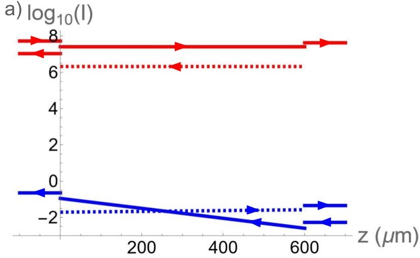
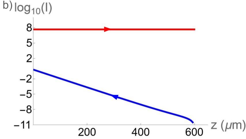
For the inset figure, was varied to vary at . For Figure 3, we used the same , , , , and . For Figure 3a, we used
| (S79a) | ||||
| (S79b) | ||||
| (S79c) | ||||
for Fig. 3b we use the same index of refraction but V/nm.
IV Spontaneous Axion Scattering
Let us consider the spontaneous generation of the Stokes field in the presence of a pump field and a fluctuating (AFM order). We include in our equation of motion for a Langevin noise term [8, 9, 10], so that the equation of motion is
| (S80) |
which, when plugging in our expression for the counter-propagating electromagnetic waves and and working in the slowly varying envelope approximation, gives
| (S81) |
Let us further simplify by neglecting terms proprotional to and considering the response on resonance, i.e. ,
| (S82) |
In the absence of this is easily solved by writing and integrating over time. The resulting solution is
| (S83) |
where we have used the fact that . Let us partition our sample into rectangles of length and cross sectional area , with the value of and in the th rectangle denoted and respectively. The correlator is then
| (S84) |
if we assume the correlations of the Langevin noise take the form
| (S85) |
we then have for the correlator of
| (S86) |
The fluctuations of can be estimated as follows: the dynamical axion field inside each box, , has average energy density
| (S87) |
The total average energy of each box is then . By the equipartition theorem, each term contributes an energy , and we therefore estimate
| (S88) |
which gives us for
| (S89) |
writing the correlator for the Langevin noise in the continuum limit, we have
| (S90) |
where we have written and
| (S91) |
For the consideration of quantum fluctuations, one can replace with , where is the occupation number of magnons, and is therefore given by
| (S92) |
Note that reduces to the expression for thermal fluctuations in the limit . We now solve the equations for and , considering to be constant in space and time. The relevant equations are
| (S93a) | |||
| (S93b) | |||
for simplicity, we write
| (S94a) | ||||
| (S94b) | ||||
and change variables to where which allows us to write our equations
| (S95a) | ||||
| (S95b) | ||||
We now Laplace transform both equations in coordinate , , using the notation
| (S96a) | ||||
| (S96b) | ||||
| (S96c) | ||||
to obtain
| (S97a) | ||||
| (S97b) | ||||
Plugging the former into the latter we can solve for
| (S98) |
which we then plug into the equation for to obtain
| (S99) |
Taking the inverse Laplace transform of Eq. (S99), we make use of the following two identities:
| (S100a) | ||||
| (S100b) | ||||
where is the th order modified Bessel function and and are the inverse Laplace transforms of and . Using identities Eqs. (S100), we find for
| (S101) |
Let us set and use the fact that , as we know will grow from to . We can then multiply the above equation by its complex conjugate and do a statistical average to obtain
| (S102) |
where we have assumed that is not correlated with , , or itself at different times, and that . To simplify Eq. (IV) we use Eq. (S90) and the continuum version of Eq. (S86),
| (S103) |
giving
| (S104) |
At long times the first term can be neglected. To see this, we use that at large arguments the modified Bessel functions can be written
| (S105a) | ||||
| (S105b) | ||||
Thus, when paired with the exponential the first term of Eq. (IV) will always go to zero in the long time limit. To see that the third term is finite, we change variables to ,
| (S106) |
in the limit that , or , we have
| (S107) |
we can rewrite
| (S108) |
where we have used the expression for on resonance. The average Stokes intensity at is then
| (S109) |
with
| (S110) |
where we have used GHz, meV, as well as using a sample size mm2 and meV. We note however that Eq. (S109) is valid under the assumption that is constant, and thus Eq. (S109) is only valid when .
References
- Bayrakci et al. [2013] S. P. Bayrakci, D. A. Tennant, P. Leininger, T. Keller, M. C. R. Gibson, S. D. Wilson, R. J. Birgeneau, and B. Keimer, Lifetimes of Antiferromagnetic Magnons in Two and Three Dimensions: Experiment, Theory, and Numerics, Physical Review Letters 111, 017204 (2013), publisher: American Physical Society.
- Li et al. [2010] R. Li, J. Wang, X.-L. Qi, and S.-C. Zhang, Dynamical axion field in topological magnetic insulators, Nature Physics 6, 284 (2010), number: 4 Publisher: Nature Publishing Group.
- Sekine and Nomura [2016] A. Sekine and K. Nomura, Chiral Magnetic Effect and Anomalous Hall Effect in Antiferromagnetic Insulators with Spin-Orbit Coupling, Physical Review Letters 116, 096401 (2016), publisher: American Physical Society.
- Zhang et al. [2009] H. Zhang, C.-X. Liu, X.-L. Qi, X. Dai, Z. Fang, and S.-C. Zhang, Topological insulators in Bi2Se3, Bi2Te3 and Sb2Te3 with a single Dirac cone on the surface, Nature Physics 5, 438 (2009), number: 6 Publisher: Nature Publishing Group.
- Boyd [2020] R. W. Boyd, ed., Nonlinear Optics (Academic Press, 2020).
- Sekine and Nomura [2021] A. Sekine and K. Nomura, Axion electrodynamics in topological materials, Journal of Applied Physics 129, 141101 (2021).
- Born and Wolf [1999] M. Born and E. Wolf, Principles of Optics: Electromagnetic Theory of Propagation, Interference and Diffraction of Light, 7th ed. (Cambridge University Press, Cambridge, 1999).
- von Foerster and Glauber [1971] T. von Foerster and R. J. Glauber, Quantum Theory of Light Propagation in Amplifying Media, Physical Review A 3, 1484 (1971), publisher: American Physical Society.
- Raymer and Mostowski [1981] M. G. Raymer and J. Mostowski, Stimulated Raman scattering: Unified treatment of spontaneous initiation and spatial propagation, Physical Review A 24, 1980 (1981), publisher: American Physical Society.
- Boyd et al. [1990] R. W. Boyd, K. Rzaewski, and P. Narum, Noise initiation of stimulated Brillouin scattering, Physical Review A 42, 5514 (1990), publisher: American Physical Society.