Mahler measure of a nonreciprocal family of elliptic curves

Detchat Samart Department of Mathematics, Faculty of Science, Burapha University, Chonburi, Thailand 20131 petesamart@gmail.com

Abstract.

In this article, we study the logarithmic Mahler measure of the one-parameter family

Q_{\alpha}=y^{2}+(x^{2}-\alpha x)y+x,

denoted by $\mathrm{m}(Q_{\alpha})$ . The zero loci of $Q_{\alpha}$ generically define elliptic curves $E_{\alpha}$ which are $3$ -isogenous to the family of Hessian elliptic curves. We are particularly interested in the case $\alpha\in(-1,3)$ , which has not been considered in the literature due to certain subtleties. For $\alpha$ in this interval, we establish a hypergeometric formula for the (modified) Mahler measure of $Q_{\alpha}$ , denoted by $\tilde{n}(\alpha).$ This formula coincides, up to a constant factor, with the known formula for $\mathrm{m}(Q_{\alpha})$ with $|\alpha|$ sufficiently large. In addition, we verify numerically that if $\alpha^{3}$ is an integer, then $\tilde{n}(\alpha)$ is a rational multiple of $L^{\prime}(E_{\alpha},0)$ . A proof of this identity for $\alpha=2$ , which is corresponding to an elliptic curve of conductor $19$ , is given.

1. Introduction

For any Laurent polynomial $P\in\mathbb{C}[x_{1}^{\pm 1},\ldots,x_{n}^{\pm 1}]\backslash\{0\}$ , the (logarithmic) Mahler measure of $P$ , denoted by $\mathrm{m}(P)$ , is the average of $\log|P|$ over the $n$ -torus. In other words,

\displaystyle\mathrm{m}(P)

\displaystyle=\frac{1}{(2\pi i)^{n}}\idotsint\limits_{|x_{1}|=\dots=|x_{n}|=1}\log|P(x_{1},\dots,x_{n})|\frac{\mathrm{d}x_{1}}{x_{1}}\dotsb\frac{\mathrm{d}x_{n}}{x_{n}}.

Consider the following two families of bivariate polynomials

	$\displaystyle P_{\alpha}(x,y)$	$\displaystyle=x^{3}+y^{3}+1-\alpha xy,$
	$\displaystyle Q_{\alpha}(x,y)$	$\displaystyle=y^{2}+(x^{2}-\alpha x)y+x,$

with the parameter $\alpha\in\mathbb{C}$ . For $\alpha\neq 3,$ the zero loci of $P_{\alpha}$ define a family of elliptic curves known as the Hessian curves. There is a $3$ -isogeny between $P_{\alpha}(x,y)=0$ and the curve

E_{\alpha}:Q_{\alpha}(x,y)=0,

which is isomorphic to the curve in the Deuring form, defined by the zero locus of

R_{\alpha}(x,y)=y^{2}+\alpha xy+y-x^{3}.

Observe that

(x^{2}y)^{3}P_{\alpha}\left(\frac{y}{x^{2}},\frac{1}{xy}\right)=Q_{\alpha}(x^{3},y^{3}),

from which we have $\mathrm{m}(P_{\alpha})=\mathrm{m}(Q_{\alpha})$ (see [20, Cor. 8]). Similarly, the change of variables $(x,y)\mapsto(-y,xy)$ transforms the family $R_{\alpha}$ into $Q_{\alpha}$ without changing the Mahler measure. For some technical reasons which shall be addressed below, we will focus on the family $Q_{\alpha}$ only. Following notation in previous papers [13, 17, 18], we let

n(\alpha):=\mathrm{m}(Q_{\alpha}).

The Mahler measure of $Q_{\alpha}$ (and its allies) was first studied by Boyd in his seminal paper [4]. He verified numerically that for several $\alpha\in\mathbb{Z}$ with $\alpha\notin(-1,3),$

(1.1)

n(\alpha)\stackrel{{\scriptstyle?}}{{=}}r_{\alpha}L^{\prime}(E_{\alpha},0),

where $r_{\alpha}\in\mathbb{Q}$ and $A\stackrel{{\scriptstyle?}}{{=}}B$ means $A$ and $B$ are equal to at least $50$ decimal places. Later, Rodriguez Villegas [23] made an observation that (1.1) seems to hold for all sufficiently large $|\alpha|$ which is a cube root of an integer. The values of $\alpha$ for which (1.1) has been proven rigorously are given in Table 1.

$\alpha$	Conductor of $E_{\alpha}$	$r_{\alpha}$	Reference(s)
$-6$	$27$	$3$	[23]
$-3$	$54$	$1$	[7]
$-2$	$35$	$1$	[7]
$-1$	$14$	$2$	[15],[7]
$\sqrt[3]{32}$	$20$	$\frac{8}{3}$	[18]
$\sqrt[3]{54}$	$36$	$\frac{3}{2}$	[17]
$5$	$14$	$7$	[15]

Table 1. Proven formulas for (1.1)

In addition to the results in this list, there are some known identities which relate $n(\alpha)$ , where $\alpha$ is a cube root of an algebraic integer, to a linear combination of $L$ -values. For example, the author proved in [19] that the following identity is true:

(1.2)

n\left(\sqrt[3]{6-6\sqrt[3]{2}+18\sqrt[3]{4}}\right)=\frac{1}{2}\left(L^{\prime}(F_{108},0)+L^{\prime}(F_{36},0)-3L^{\prime}(F_{27},0)\right),

where $F_{N}$ is an elliptic curve over $\mathbb{Q}$ of conductor $N$ . In compliance with Boyd’s results, it is worth noting that

\sqrt[3]{6-6\sqrt[3]{2}+18\sqrt[3]{4}}\approx 3.0005>3.

We refer the interested reader to the aforementioned paper for more conjectural identities of this type.

Recall that a polynomial $P(x_{1},x_{2},\ldots,x_{n})$ is said to be reciprocal if there exist integers $d_{1},d_{2},\ldots,d_{n}$ such that

x_{1}^{d_{1}}x_{2}^{d_{2}}\cdots x_{n}^{d_{n}}P(1/x_{1},1/x_{2},\ldots,1/x_{n})=P(x_{1},x_{2},\ldots,x_{n}),

and nonreciprocal otherwise. For a family of two-variable polynomials

(1.3)

\tilde{P}_{\alpha}(x,y)=A(x)y^{2}+(B(x)+\alpha x)y+C(x),

let $Z_{\alpha}$ be the zero locus of $\tilde{P}_{\alpha}(x,y)$ and let $K$ be the set of $\alpha\in\mathbb{C}$ for which $\tilde{P}_{\alpha}$ vanishes on the $2$ -torus. Boyd conjectured from his experiments that, for all integer $\alpha$ in the unbounded component $G_{\infty}$ of $\mathbb{C}\backslash K$ , if $\tilde{P}_{\alpha}$ is tempered (see [23] for the definition), then $\mathrm{m}(\tilde{P}_{\alpha})$ is related to an $L$ -value of elliptic curve (if $Z_{\alpha}$ has genus one) or Dirichlet character (if $Z_{\alpha}$ has genus zero). If $\tilde{P}_{\alpha}(x,y)$ is reciprocal, then it can be shown that $K\subseteq\mathbb{R}$ , implying $\overline{G}_{\infty}=\mathbb{C}$ . Hence by continuity one could expect that identities like (1.1) hold for all $\alpha\in\mathbb{Z}$ , with some exceptions in the genus zero cases. Examples of polynomials satisfying these properties include the families $x+1/x+y+1/y+\alpha$ and $(1+x)(1+y)(x+y)-\alpha xy$ , whose Mahler measures have been extensively studied over the past few decades (e.g. see [4, 12, 13, 14, 15, 17, 18, 23]).

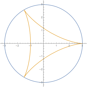
The family $Q_{\alpha}$ , on the other hand, is nonreciprocal, so the set $K$ of $\alpha\in\mathbb{C}$ for which $Q_{\alpha}$ vanishes on the $2$ -torus has nonempty interior. In fact, as described in [4, §2B] and [23, §14], $K$ is the region inside a hypocycloid whose vertices are the cube roots of $27$ in the complex plane and $K\cap\mathbb{R}=(-1,3)$ . This is illustrated in Figure 1 below.

It is known (see, for example, [17, Thm. 3.1]) that, for most complex numbers $\alpha$ , $n(\alpha)$ is expressible in terms of a generalized hypergeometric function: if $|\alpha|$ is sufficiently large, then

(1.4)

n(\alpha)=\mathop{\mathrm{Re}}\left(\log\alpha-\frac{2}{\alpha^{3}}{}_{4}F_{3}\biggl{(}\genfrac{.}{.}{0.0pt}{}{\frac{4}{3}\mathchar 44\relax\mkern 6.0mu\frac{5}{3}\mathchar 44\relax\mkern 6.0mu1\mathchar 44\relax\mkern 6.0mu1}{2\mathchar 44\relax\mkern 6.0mu2\mathchar 44\relax\mkern 6.0mu2}\,\,\bigg{|}\,\,\frac{27}{\alpha^{3}}\biggr{)}\right).

Since both sides of (1.4) are real parts of holomorphic functions that agree at every point in an open subset of the region $\mathbb{C}\backslash K$ , the formula (1.4) is valid for all $\alpha\in\mathbb{C}\backslash K;$ i.e., for all $\alpha$ on the border and outside of the hypocycloid in Figure 1. Because of this anomalous property of the family $Q_{\alpha}$ (and other nonreciprocal families in general), to our knowledge, there are no known results about $n(\alpha)$ for $\alpha\in K$ , with an exception for the case $\alpha=0$ due to Smyth [21], namely

n(0)=\mathrm{m}(x^{3}+y^{3}+1)=\mathrm{m}(x+y+1)=L^{\prime}(\chi_{-3},-1),

where $\chi_{-N}=\left(\frac{N}{\cdot}\right).$ The aim of this paper is to give a thorough investigation of these omitted values of $n(\alpha)$ . In particular, we are interested in establishing formulas analogous to (1.1) and (1.4) for $\alpha\in(-1,3)$ .

While the family $P_{\alpha}$ is more well established than the family $Q_{\alpha}$ in the literature, we choose to work with the latter for the following two reasons. Firstly, the family $Q_{\alpha}$ is in the form (1.3), whose Mahler measure can be efficiently computed from both theoretical and numerical perspectives, regardless of the value of $\alpha$ . Therefore, one can test the results numerically with high precision computations. The Mahler measure of $P_{\alpha}$ , on the other hand, is quite difficult to compute, especially when $\alpha\in K$ . Secondly, although the zero loci of $P_{\alpha}$ and $Q_{\alpha}$ give elliptic curves in the same isogeny class, their certain arithmetic properties, which are involved in the process of evaluating their Mahler measure in terms of $L^{\prime}(E_{\alpha},0)$ , could be different. This will be elaborated at the end of this section.

Let us first factorize $Q_{\alpha}$ as

Q_{\alpha}(x,y)=y^{2}+(x^{2}-\alpha x)y+x=(y-y_{+}(x))(y-y_{-}(x)),

where

y_{\pm}(x)=-(x^{2}-\alpha x)\left(\frac{1}{2}\pm\sqrt{\frac{1}{4}-\frac{1}{x(x-\alpha)^{2}}}\right),

and denote

J(\alpha)=\frac{1}{\pi}\int_{\cos^{-1}\left(\frac{\alpha-1}{2}\right)}^{\pi}\log|y_{+}(e^{i\theta})|\mathrm{d}\theta.

(Here and throughout we use the principal branch for the complex square root.) The significance of the function $J(\alpha)$ , which can be seen as a part of $\mathrm{m}(Q_{\alpha})$ , will be made clear later. For $\alpha\in(-1,1)\cup(1,3)$ , $y_{\pm}(x)$ are functions on $\mathbb{T}^{1}:=\{x\in\mathbb{C}\mid|x|=1\}$ . If $\alpha=1$ , $y_{\pm}(x)$ have only one removable singularity on $\mathbb{T}^{1}$ , namely $x=1$ , so we can extend its domain to $\mathbb{T}^{1}$ by setting

y_{\pm}(1)=\lim_{x\rightarrow 1}y_{\pm}(x)=\mp i.

The first main result of this paper is the following hypergeometric formula, which extends (1.4).

Theorem 1.

Let $\tilde{n}(\alpha)=n(\alpha)-3J(\alpha)$ . For $\alpha\in(-1,3)\backslash\{0\}$ , the following identity is true:

\tilde{n}(\alpha)=\frac{4}{1-3\,\mathrm{sgn}(\alpha)}\mathop{\mathrm{Re}}\left(\log\alpha-\frac{2}{\alpha^{3}}{}_{4}F_{3}\biggl{(}\genfrac{.}{.}{0.0pt}{}{\frac{4}{3}\mathchar 44\relax\mkern 6.0mu\frac{5}{3}\mathchar 44\relax\mkern 6.0mu1\mathchar 44\relax\mkern 6.0mu1}{2\mathchar 44\relax\mkern 6.0mu2\mathchar 44\relax\mkern 6.0mu2}\,\,\bigg{|}\,\,\frac{27}{\alpha^{3}}\biggr{)}\right).

By Theorem 1 and a result of Rogers [17, Eq. (43)], we can express $\tilde{n}(\alpha)$ in terms of (convergent) ${}_{3}F_{2}$ -hypergeometric series; for $\alpha\in(-1,3)\backslash\{0\}$ ,

\tilde{n}(\alpha)=s(\alpha)\left(\frac{\sqrt[3]{2}\Gamma\left(\frac{1}{6}\right)\Gamma\left(\frac{1}{3}\right)\Gamma\left(\frac{1}{2}\right)}{\sqrt{3}\pi^{2}}\alpha{}_{3}F_{2}\biggl{(}\genfrac{.}{.}{0.0pt}{}{\frac{1}{3}\mathchar 44\relax\mkern 6.0mu\frac{1}{3}\mathchar 44\relax\mkern 6.0mu\frac{1}{3}}{\frac{2}{3}\mathchar 44\relax\mkern 6.0mu\frac{4}{3}}\,\,\bigg{|}\,\,\frac{\alpha^{3}}{27}\biggr{)}+\frac{\Gamma^{3}\left(\frac{2}{3}\right)}{2\pi^{2}}\alpha^{2}{}_{3}F_{2}\biggl{(}\genfrac{.}{.}{0.0pt}{}{\frac{2}{3}\mathchar 44\relax\mkern 6.0mu\frac{2}{3}\mathchar 44\relax\mkern 6.0mu\frac{2}{3}}{\frac{4}{3}\mathchar 44\relax\mkern 6.0mu\frac{5}{3}}\,\,\bigg{|}\,\,\frac{\alpha^{3}}{27}\biggr{)}\right),

where $s(\alpha)=-\frac{(1+3\,\mathrm{sgn}(\alpha))^{2}}{64}.$

We also study $\tilde{n}(\alpha)$ from the arithmetic point of view. We discovered from our numerical computation that when $\alpha\in(-1,3)$ is a cube root of an integer, then $\tilde{n}(\alpha)$ (conjecturally) satisfies an identity analogous to (1.1). Numerical data for this identity are given in Table 2. This identity can be proven rigorously in some cases using Brunault-Mellit-Zudilin’s formula (see Theorem 8 below). As a concrete example, we prove the following result.

Theorem 2.

Let $\tilde{n}(\alpha)=n(\alpha)-3J(\alpha)$ and let $E_{\alpha}$ be the elliptic curve defined by the zero locus of $Q_{\alpha}$ . Then the following evaluation is true:

(1.5)

\displaystyle\tilde{n}(2)

\displaystyle=-3L^{\prime}(E_{2},0).

Note that $E_{2}$ has conductor $19$ . What makes this curve special is that it admits a modular unit parametrization. The celebrated modularity theorem asserts that every elliptic curve over $\mathbb{Q}$ can be parametrized by modular functions. However, a recent result of Brunault [6] reveals that there are only a finite number of them which can be parametrized by modular units (i.e. modular functions whose zeros and poles are supported at the cusps). In order to apply Brunault-Mellit-Zudilin’s formula, one needs to show that the integration path corresponding to $\tilde{n}(2)$ becomes a closed path for the regulator integral defined on the curve $Q_{2}(x,y)=0.$ This path can then be translated into a path joining cusps on the modular curve $X_{1}(19)$ . The calculation for this part will be worked out in Section 3. On the other hand, the isogenous curve $P_{2}(x,y)=0$ , which has Cremona label $19a1$ , does not admit such a nice parametrization [6, Tab. 1], so we cannot use the same argument to directly relate $\mathrm{m}(P_{2})$ to $L^{\prime}(E_{2},0).$

2. The hypergeometric formula

The goal of this section is to prove Theorem 1. To achieve this goal, we need some auxiliary results as follows.

Lemma 3.

Let $\alpha\in\mathbb{C}$ and $x\in\mathbb{C}\backslash\{\alpha\}$ . If $|x|=1$ , then $|y_{-}(x)|\leq 1\leq|y_{+}(x)|.$

Proof.

Assume that $|x|=1$ and write $\sqrt{\frac{1}{4}-\frac{1}{x(x-\alpha)^{2}}}=a+bi$ , where $a,b\in\mathbb{R}.$ Since the square root is defined using the principal branch, we have $a\geq 0$ . Hence

|y_{-}(x)|=|x^{2}-\alpha x|\left|\frac{1}{2}-a-bi\right|\leq|x^{2}-\alpha x|\left|\frac{1}{2}+a+bi\right|=|y_{+}(x)|.

Since $|y_{+}(x)||y_{-}(x)|=|x|=1$ , it follows that $|y_{-}(x)|\leq 1\leq|y_{+}(x)|$ , as desired. ∎

By Lemma 3 and Jensen’s formula, we have

(2.1)	$\displaystyle n(\alpha)$	$\displaystyle=\frac{1}{2\pi}\int_{-\pi}^{\pi}\log\|y_{+}(e^{i\theta})\|\mathrm{d}\theta$
		$\displaystyle=\frac{1}{\pi}\int_{0}^{\pi}\log\|y_{+}(e^{i\theta})\|\mathrm{d}\theta$
		$\displaystyle=\frac{1}{\pi}\mathop{\mathrm{Re}}\int_{0}^{\pi}\log\left((x-\alpha)\left(\frac{1}{2}+\sqrt{\frac{1}{4}-\frac{1}{x(x-\alpha)^{2}}}\right)\right)\bigg{\rvert}_{x=e^{i\theta}}\mathrm{d}\theta,$

where the second equality follows from $y_{+}(e^{-i\theta})=\overline{y_{+}(e^{i\theta})}.$ Next, we shall locate the toric points, the points of intersection of the affine curve $Q_{\alpha}=0$ and the $2$ -torus, explicitly.

Proposition 4.

Let $\mathbb{T}^{2}=\{(x,y)\in\mathbb{C}^{2}\mid|x|=|y|=1\}$ and for each $\alpha\in\mathbb{C}$ let $C_{\alpha}=\{(x,y)\in\mathbb{C}^{2}\mid Q_{\alpha}(x,y)=0\}$ . Then for $\alpha\in(-1,3)$ , we have

C_{\alpha}\cap\mathbb{T}^{2}=\left\{\left(e^{it},y_{\pm}(e^{it})\right)\mid t=0,\pm\cos^{-1}\left(\frac{\alpha-1}{2}\right)\right\}.

Proof.

Assume first that $\alpha\neq 1$ . Suppose $|x|=1$ , so $x=e^{it}$ for some $t\in(-\pi,\pi].$ Since $y_{\pm}(x)=-(x^{2}-\alpha x)\left(\frac{1}{2}\pm\sqrt{\frac{1}{4}-\frac{1}{x(x-\alpha)^{2}}}\right)$ and $|y_{+}(x)||y_{-}(x)|=|x|=1$ , we have that the condition $|y_{+}(x)|=1=|y_{-}(x)|$ is equivalent to the equality

(2.2)

\left|\frac{1}{2}+\sqrt{\frac{1}{4}-\frac{1}{x(x-\alpha)^{2}}}\right|=\left|\frac{1}{2}-\sqrt{\frac{1}{4}-\frac{1}{x(x-\alpha)^{2}}}\right|.

It is easily seen that (2.2) holds if and only if $\sqrt{\frac{1}{4}-\frac{1}{x(x-\alpha)^{2}}}$ is purely imaginary; equivalently, $x(x-\alpha)^{2}\in(0,4)$ . Simple calculation yields

(2.3)	$\displaystyle\mathop{\mathrm{Re}}(x(x-\alpha)^{2})$	$\displaystyle=(\cos t)((\cos t-\alpha)^{2}-\sin^{2}t)-2(\cos t-\alpha)\sin^{2}t,$
(2.4)	$\displaystyle\mathop{\mathrm{Im}}(x(x-\alpha)^{2})$	$\displaystyle=(\sin t)(2\cos t-(\alpha-1))(2\cos t-(\alpha+1)),$
(2.5)	$\displaystyle\|x(x-\alpha)^{2}\|$	$\displaystyle=\|x-\alpha\|^{2}=\alpha^{2}-2\alpha\cos t+1.$

We have from (2.4) that $x(x-\alpha)^{2}\in\mathbb{R}$ if and only if $\sin t=0$ or $\cos t=(\alpha\pm 1)/2.$
If $\sin t=0$ , then either $\cos t=1$ or $\cos t=-1.$ If $\cos t=-1$ , then $x(x-\alpha)^{2}=-(1+\alpha)^{2}<0.$ If $\cos t=(\alpha+1)/2$ , then $\alpha\in(-1,1)$ and $\sin^{2}t=1-\left((\alpha+1)/2\right)^{2},$ from which we can deduce using (2.3) that

x(x-\alpha)^{2}=\mathop{\mathrm{Re}}(x(x-\alpha)^{2})=\alpha-1<0.

Also, it can be shown using (2.3) and (2.5) that the remaining cases, $\cos t=1$ and $\cos t=\frac{\alpha-1}{2}$ , imply $0<x(x-\alpha)^{2}<4$ . As a consequence, the curve $C_{\alpha}=0$ intersects $\mathbb{T}^{2}$ exactly at $\left(e^{it},y_{\pm}(e^{it})\right)$ , where $t=0,\pm\cos^{-1}\left(\frac{\alpha-1}{2}\right)$ . The same result also holds for $\alpha=1$ by continuity. ∎

Lemma 5.

For $\lambda\in[1,2)$ , let $p_{\lambda}(x)=x(\lambda^{2}-x)\left(x^{2}+\left(\frac{4}{\lambda}-\lambda^{2}\right)x+\frac{4}{\lambda^{2}}\right)$ and $\gamma=\frac{\lambda^{3}-\lambda-2}{2\lambda}+\frac{\lambda+1}{2\lambda}\sqrt{(2-\lambda)(\lambda^{3}+\lambda-2)}i$ . Then we have

(2.6)

\int_{\lambda-1}^{\gamma}\frac{1}{\sqrt{-p_{\lambda}(x)}}\mathrm{d}x=\int_{0}^{-1/\lambda}\frac{1}{\sqrt{-p_{\lambda}(x)}}\mathrm{d}x,

where the left (complex) integral is path-independent in the upper-half unit disk and the right integral is a real integral.

Proof.

Note first that $|\gamma|=1$ and the nonzero roots of $p_{\lambda}(x)$ are

x_{1}(\lambda)=\lambda^{2},\quad x_{2}(\lambda)=\frac{\lambda^{3}-4+\sqrt{\lambda^{3}(\lambda^{3}-8)}}{2\lambda},\text{ and }x_{3}(\lambda)=\frac{\lambda^{3}-4-\sqrt{\lambda^{3}(\lambda^{3}-8)}}{2\lambda},

which lie outside the unit circle, so the integration path for the left integral can be chosen to be any path joining $\lambda-1$ and $\gamma$ in the upper-half unit disk. For $1<\lambda<2$ and $x\in\mathbb{R}$ ,

x^{2}+\left(\frac{4}{\lambda}-\lambda^{2}\right)x+\frac{4}{\lambda^{2}}=\left(x+\left(\frac{2}{\lambda}-\frac{\lambda^{2}}{2}\right)\right)^{2}-\lambda\left(\frac{\lambda^{3}}{4}-2\right)>0,

so $-p_{\lambda}(x)>0$ for all $x\in(-1/\lambda,0)$ and the integral on the right-hand side is real. Define the symmetric polynomial¹¹1We obtain the polynomial $F_{\lambda}(x,y)$ using numerical values of the integrals in (2.6). The PSLQ algorithm plays an essential role in identifying its coefficients. $F_{\lambda}(x,y)$ by

F_{\lambda}(x,y):=\lambda^{2}(\lambda-1)x^{2}y^{2}-\lambda(\lambda-1)(\lambda^{3}-\lambda^{2}+\lambda-2)(x^{2}y+xy^{2})+\lambda^{2}(x^{2}+y^{2})\\ +(\lambda^{7}-2\lambda^{6}+2\lambda^{5}-5\lambda^{4}+6\lambda^{3}-6\lambda^{2}+6\lambda-4)xy-2\lambda^{2}(\lambda-1)(x+y)+\lambda^{2}(\lambda-1)^{2}.

Then, for $\lambda\in[1,2)$ , $F_{\lambda}(x,y)$ transforms the interval $(-1/\lambda,0)$ to a continuous path in the upper-half unit disk joining $\gamma$ and $\lambda-1$ . Moreover, by implicitly differentiating $F_{\lambda}(x,y)=0$ , it can be checked using a computer algebra system that the following equation holds on this curve:

\left(\frac{\mathrm{d}y}{\mathrm{d}x}\right)^{2}-\frac{p_{\lambda}(y)}{p_{\lambda}(x)}=0,

from which (2.6) follows immediately. ∎

Lemma 6.

For $\alpha\in(-1,3),$ if $\alpha=(\lambda^{3}-2)/\lambda$ , then

\frac{\mathrm{d}}{\mathrm{d}\alpha}\left(n(\alpha)-3J(\alpha)\right)=-\frac{1}{\pi}\int_{0}^{\lambda^{2}}\frac{1}{\sqrt{p_{\lambda}(x)}}\mathrm{d}x,

where $p_{\lambda}(x)$ is defined as in Lemma 5.

Proof.

Differentiating (2.1) with respect to $\alpha$ yields

\frac{\mathrm{d}}{\mathrm{d}\alpha}n(\alpha)=\frac{1}{\pi}\mathop{\mathrm{Re}}\int_{0}^{\pi}\frac{\sqrt{x}}{\sqrt{x(x-\alpha)^{2}-4}}\bigg{\rvert}_{x=e^{i\theta}}\mathrm{d}\theta.

Let $c(\alpha)=\cos^{-1}\left(\frac{\alpha-1}{2}\right)$ . Then, by Leibniz integral rule and Proposition 4, we have

	$\displaystyle\frac{\mathrm{d}}{\mathrm{d}\alpha}J(\alpha)$	$\displaystyle=\frac{1}{\pi}\Bigg{(}-\log\left\|y_{+}\left(e^{ic(\alpha)}\right)\right\|\frac{\mathrm{d}}{\mathrm{d}\alpha}c(\alpha)$
		$\displaystyle\qquad+\mathop{\mathrm{Re}}\int_{c(\alpha)}^{\pi}\frac{\mathrm{d}}{\mathrm{d}\alpha}\log\left((x-\alpha)\left(\frac{1}{2}+\sqrt{\frac{1}{4}-\frac{1}{x(x-\alpha)^{2}}}\right)\right)\bigg{\rvert}_{x=e^{i\theta}}\mathrm{d}\theta\Bigg{)}$
		$\displaystyle=\frac{1}{\pi}\mathop{\mathrm{Re}}\int_{0}^{c(\alpha)}\frac{\sqrt{x}}{\sqrt{x(x-\alpha)^{2}-4}}\bigg{\rvert}_{x=e^{i\theta}}\mathrm{d}\theta.$

It follows that

(2.7)

\frac{\mathrm{d}}{\mathrm{d}\alpha}\left(n(\alpha)-3J(\alpha)\right)=-\frac{1}{\pi}\mathop{\mathrm{Re}}\left(\left(2\int_{c(\alpha)}^{\pi}-\int_{0}^{c(\alpha)}\right)\frac{\sqrt{x}}{\sqrt{x(x-\alpha)^{2}-4}}\bigg{\rvert}_{x=e^{i\theta}}\mathrm{d}\theta\right).

Let $\alpha=(\lambda^{3}-2)/\lambda$ . Then $\alpha$ maps the interval $(1,2)$ bijectively onto $(-1,3)$ and

(2.8)

x(x-\alpha)^{2}-4=(x-\lambda^{2})\left(x^{2}+\left(\frac{4}{\lambda}-\lambda^{2}\right)x+\frac{4}{\lambda^{2}}\right).

An inspection of the signs of the square roots in the integrand reveals that

(2.9)		$\displaystyle\int_{c(\alpha)}^{\pi}\frac{\sqrt{x}}{\sqrt{x(x-\alpha)^{2}-4}}\bigg{\rvert}_{x=e^{i\theta}}\mathrm{d}\theta$	$\displaystyle=-\int_{\gamma}^{-1}\frac{1}{\sqrt{p_{\lambda}(x)}}\mathrm{d}x=\left(\int_{0}^{\gamma}-\int_{0}^{-1}\right)\frac{1}{\sqrt{p_{\lambda}(x)}}\mathrm{d}x,$
(2.10)		$\displaystyle\int_{0}^{c(\alpha)}\frac{\sqrt{x}}{\sqrt{x(x-\alpha)^{2}-4}}\bigg{\rvert}_{x=e^{i\theta}}\mathrm{d}\theta$	$\displaystyle=\int_{1}^{\gamma}\frac{1}{\sqrt{p_{\lambda}(x)}}\mathrm{d}x=\left(\int_{0}^{\gamma}-\int_{0}^{1}\right)\frac{1}{\sqrt{p_{\lambda}(x)}}\mathrm{d}x,$

where

\gamma=e^{ic(\alpha)}=\frac{\alpha-1}{2}+\frac{\sqrt{(3-\alpha)(\alpha+1)}}{2}i=\frac{\lambda^{3}-\lambda-2}{2\lambda}+\frac{\lambda+1}{2\lambda}\sqrt{(2-\lambda)(\lambda^{3}+\lambda-2)}i.

Since $p_{\lambda}(x)<0$ for any $x\in(-1,0)$ and $\lambda\in(1,2)$ , we have

(2.11)

\mathop{\mathrm{Re}}\int_{0}^{-1}\frac{1}{\sqrt{p_{\lambda}(x)}}\mathrm{d}x=0.

Plugging (2.9),(2.10), and (2.11) into (2.7) gives

(2.12)

\frac{\mathrm{d}}{\mathrm{d}\alpha}\left(n(\alpha)-3J(\alpha)\right)=-\frac{1}{\pi}\left(\int_{0}^{1}\frac{1}{\sqrt{p_{\lambda}(x)}}\mathrm{d}x+\mathop{\mathrm{Re}}\int_{0}^{\gamma}\frac{1}{\sqrt{p_{\lambda}(x)}}\mathrm{d}x\right).

Note that the mapping

(2.13)

x\mapsto\frac{\lambda^{2}-x}{\lambda x+1}

is the unique Möbius transformation which interchanges the following values:

0\leftrightarrow\lambda^{2},\quad 1\leftrightarrow\lambda-1,\quad x_{2}(\lambda)\leftrightarrow x_{3}(\lambda),

where $x_{2}(\lambda)$ and $x_{3}(\lambda)$ are the roots of $x^{2}+(4/\lambda-\lambda^{2})x+4/\lambda^{2}$ . Hence using (2.13) we have

\int_{0}^{\lambda-1}\frac{1}{\sqrt{p_{\lambda}(x)}}\mathrm{d}x=\int_{1}^{\lambda^{2}}\frac{1}{\sqrt{p_{\lambda}(x)}}\mathrm{d}x.

Finally, we have from Lemma 5 that

\int_{\lambda-1}^{\gamma}\frac{1}{\sqrt{p_{\lambda}(x)}}\mathrm{d}x=\int_{0}^{-1/\lambda}\frac{1}{\sqrt{p_{\lambda}(x)}}\mathrm{d}x\in i\mathbb{R},

so (2.12) immediately gives the desired result. ∎

Lemma 7.

For $\alpha\in(-1,0)$ , we have

(2.14)

\frac{\mathrm{d}}{\mathrm{d}\alpha}\left(n(\alpha)-3J(\alpha)\right)=\mathop{\mathrm{Re}}\left(\frac{1}{\alpha}{}_{2}F_{1}\biggl{(}\genfrac{.}{.}{0.0pt}{}{\frac{1}{3}\mathchar 44\relax\mkern 6.0mu\frac{2}{3}}{1}\,\,\bigg{|}\,\,\frac{27}{\alpha^{3}}\biggr{)}\right).

For $\alpha\in(0,3)$ , we have

(2.15)

\frac{\mathrm{d}}{\mathrm{d}\alpha}\left(n(\alpha)-3J(\alpha)\right)=-2\mathop{\mathrm{Re}}\left(\frac{1}{\alpha}{}_{2}F_{1}\biggl{(}\genfrac{.}{.}{0.0pt}{}{\frac{1}{3}\mathchar 44\relax\mkern 6.0mu\frac{2}{3}}{1}\,\,\bigg{|}\,\,\frac{27}{\alpha^{3}}\biggr{)}\right).

Proof.

Let us first consider (2.15). We prove this identity by expressing both sides in terms of the elliptic integral of the first kind

K(z)=\int_{0}^{1}\frac{\mathrm{d}x}{\sqrt{(1-x^{2})(1-z^{2}x^{2})}}.

Again, let $\alpha=(\lambda^{3}-2)/\lambda.$ Following a procedure in [11, Ch. 3], we let

u=\frac{-1-\sqrt{\lambda^{3}+1}}{\lambda},\quad v=\frac{-1+\sqrt{\lambda^{3}+1}}{\lambda},\quad x=\frac{ut-v}{t-1}.

This substitution transforms the integral in Lemma 6 (without the factor $-1/\pi$ ) into

\frac{\lambda}{2\sqrt{\lambda^{3}+1}}\int_{t_{1}}^{t_{2}}\frac{\mathrm{d}t}{\sqrt{(B_{1}t^{2}+A_{1})(B_{2}t^{2}+A_{2})}},

where

$\displaystyle t_{1}$	$\displaystyle=-\frac{\lambda^{3}+2-2\sqrt{\lambda^{3}+1}}{\lambda^{3}},$	$\displaystyle t_{2}=-t_{1},$
$\displaystyle A_{1}$	$\displaystyle=\frac{\lambda^{3}+2-2\sqrt{\lambda^{3}+1}}{4\sqrt{\lambda^{3}+1}},$	$\displaystyle B_{1}=\frac{-\lambda^{3}-2-2\sqrt{\lambda^{3}+1}}{4\sqrt{\lambda^{3}+1}},$
$\displaystyle A_{2}$	$\displaystyle=\frac{-\lambda^{3}+2+2\sqrt{\lambda^{3}+1}}{4\sqrt{\lambda^{3}+1}},$	$\displaystyle B_{2}=\frac{\lambda^{3}-2+2\sqrt{\lambda^{3}+1}}{4\sqrt{\lambda^{3}+1}}.$

Observe that, for $\lambda\in(1,2)$ , we have $A_{1},A_{2},B_{2}>0$ , $B_{1}<0$ , and $\sqrt{-A_{1}/B_{1}}=t_{2}.$ Hence the substitution $t\mapsto\sqrt{-A_{1}/B_{1}}t$ yields

	$\displaystyle\frac{\lambda}{2\sqrt{\lambda^{3}+1}}\int_{t_{1}}^{t_{2}}\frac{\mathrm{d}t}{\sqrt{(B_{1}t^{2}+A_{1})(B_{2}t^{2}+A_{2})}}$	$\displaystyle=\frac{\lambda}{2\sqrt{\lambda^{3}+1}}\sqrt{-\frac{1}{A_{2}B_{1}}}\int_{-1}^{1}\frac{\mathrm{d}t}{\sqrt{(1-t^{2})\left(1-\frac{A_{1}B_{2}}{A_{2}B_{1}}t^{2}\right)}}$
		$\displaystyle=\frac{4\lambda}{\sqrt{\left(\sqrt{\lambda^{3}+1}+1\right)^{3}\left(3-\sqrt{\lambda^{3}+1}\right)}}K\left(\sqrt{\frac{A_{1}B_{2}}{A_{2}B_{1}}}\right).$

Therefore, we obtain

(2.16)

\frac{\mathrm{d}}{\mathrm{d}\alpha}\left(n(\alpha)-3J(\alpha)\right)=-\frac{4\lambda}{\pi\sqrt{\left(\sqrt{\lambda^{3}+1}+1\right)^{3}\left(3-\sqrt{\lambda^{3}+1}\right)}}K\left(\sqrt{\frac{A_{1}B_{2}}{A_{2}B_{1}}}\right).

On the other hand, we apply the hypergeometric transformation [18, p. 410]

(2.17)

\mathop{\mathrm{Re}}{}_{2}F_{1}\biggl{(}\genfrac{.}{.}{0.0pt}{}{\frac{1}{3}\mathchar 44\relax\mkern 6.0mu\frac{2}{3}}{1}\,\,\bigg{|}\,\,\frac{27y}{(y-2)^{3}}\biggr{)}=\frac{y-2}{y+4}{}_{2}F_{1}\biggl{(}\genfrac{.}{.}{0.0pt}{}{\frac{1}{3}\mathchar 44\relax\mkern 6.0mu\frac{2}{3}}{1}\,\,\bigg{|}\,\,\frac{27y^{2}}{(y+4)^{3}}\biggr{)},

which is valid for $y\in(2,8)$ , to write the right-hand side of (2.15) as

	$\displaystyle-\frac{2}{\alpha}\mathop{\mathrm{Re}}\left({}_{2}F_{1}\biggl{(}\genfrac{.}{.}{0.0pt}{}{\frac{1}{3}\mathchar 44\relax\mkern 6.0mu\frac{2}{3}}{1}\,\,\bigg{\|}\,\,\frac{27}{\alpha^{3}}\biggr{)}\right)$	$\displaystyle=\frac{2\lambda}{2-\lambda^{3}}\mathop{\mathrm{Re}}\left({}_{2}F_{1}\biggl{(}\genfrac{.}{.}{0.0pt}{}{\frac{1}{3}\mathchar 44\relax\mkern 6.0mu\frac{2}{3}}{1}\,\,\bigg{\|}\,\,\frac{27\lambda^{3}}{(\lambda^{3}-2)^{3}}\biggr{)}\right)$
		$\displaystyle=-\frac{2\lambda}{\lambda^{3}+4}{}_{2}F_{1}\biggl{(}\genfrac{.}{.}{0.0pt}{}{\frac{1}{3}\mathchar 44\relax\mkern 6.0mu\frac{2}{3}}{1}\,\,\bigg{\|}\,\,\frac{27\lambda^{6}}{(\lambda^{3}+4)^{3}}\biggr{)}.$

The substitution $\lambda=\sqrt[3]{4(p+p^{2})}$ gives a bijection from the interval $((\sqrt{3}-1)/2,1)$ onto $(\sqrt[3]{2},2)$ , which is corresponding to the interval $(0,3)$ for $\alpha$ , with the inverse mapping $p=(\sqrt{\lambda^{3}+1}-1)/2$ . We apply this substitution together with a classical result of Ramanujan [2, Thm 5.6] to deduce

	$\displaystyle-\frac{2\lambda}{\lambda^{3}+4}{}_{2}F_{1}\biggl{(}\genfrac{.}{.}{0.0pt}{}{\frac{1}{3}\mathchar 44\relax\mkern 6.0mu\frac{2}{3}}{1}\,\,\bigg{\|}\,\,\frac{27\lambda^{6}}{(\lambda^{3}+4)^{3}}\biggr{)}$	$\displaystyle=-\frac{\sqrt[3]{4(p+p^{2})}}{2(p^{2}+p+1)}{}_{2}F_{1}\biggl{(}\genfrac{.}{.}{0.0pt}{}{\frac{1}{3}\mathchar 44\relax\mkern 6.0mu\frac{2}{3}}{1}\,\,\bigg{\|}\,\,\frac{27p^{2}(1+p)^{2}}{4(1+p+p^{2})^{3}}\biggr{)}$
		$\displaystyle=-\frac{\sqrt[3]{4(p+p^{2})}}{2\sqrt{1+2p}}{}_{2}F_{1}\biggl{(}\genfrac{.}{.}{0.0pt}{}{\frac{1}{2}\mathchar 44\relax\mkern 6.0mu\frac{1}{2}}{1}\,\,\bigg{\|}\,\,\frac{p^{3}(2+p)}{1+2p}\biggr{)}$
		$\displaystyle=-\frac{\lambda}{2\sqrt[4]{\lambda^{3}+1}}{}_{2}F_{1}\biggl{(}\genfrac{.}{.}{0.0pt}{}{\frac{1}{2}\mathchar 44\relax\mkern 6.0mu\frac{1}{2}}{1}\,\,\bigg{\|}\,\,\rho(\lambda)\biggr{)},$

where

\rho(\lambda)=\frac{\lambda^{6}-4\lambda^{3}-8+8\sqrt{\lambda^{3}+1}}{16\sqrt{\lambda^{3}+1}}.

Then by the identities [1, Eq. 3.2.3], [9, Eq. 15.8.1]

K(k)=\frac{\pi}{2}{}_{2}F_{1}\biggl{(}\genfrac{.}{.}{0.0pt}{}{\frac{1}{2}\mathchar 44\relax\mkern 6.0mu\frac{1}{2}}{1}\,\,\bigg{|}\,\,k^{2}\biggr{)},\qquad K(\sqrt{r})=\frac{1}{\sqrt{1-r}}K\left(\sqrt{\frac{r}{r-1}}\right),

we arrive at

(2.18)

-\frac{\lambda}{2\sqrt[4]{\lambda^{3}+1}}{}_{2}F_{1}\biggl{(}\genfrac{.}{.}{0.0pt}{}{\frac{1}{2}\mathchar 44\relax\mkern 6.0mu\frac{1}{2}}{1}\,\,\bigg{|}\,\,\rho(\lambda)\biggr{)}=-\frac{4\lambda}{\pi\sqrt{\left(\sqrt{\lambda^{3}+1}+1\right)^{3}\left(3-\sqrt{\lambda^{3}+1}\right)}}K\left(\sqrt{\frac{\rho(\lambda)}{\rho(\lambda)-1}}\right).

It can be calculated directly that

\frac{\rho(\lambda)}{\rho(\lambda)-1}=\frac{\lambda^{6}-4\lambda^{3}-8+8\sqrt{\lambda^{3}+1}}{\lambda^{6}-4\lambda^{3}-8-8\sqrt{\lambda^{3}+1}}=\frac{A_{1}B_{2}}{A_{2}B_{1}},

so the right-hand side of (2.18) coincides with that of (2.16) and the proof is completed. Equation (2.14) also follows from the arguments above, provided that (2.17) is replaced with

\mathop{\mathrm{Re}}{}_{2}F_{1}\biggl{(}\genfrac{.}{.}{0.0pt}{}{\frac{1}{3}\mathchar 44\relax\mkern 6.0mu\frac{2}{3}}{1}\,\,\bigg{|}\,\,\frac{27y}{(y-2)^{3}}\biggr{)}=\frac{4-2y}{y+4}{}_{2}F_{1}\biggl{(}\genfrac{.}{.}{0.0pt}{}{\frac{1}{3}\mathchar 44\relax\mkern 6.0mu\frac{2}{3}}{1}\,\,\bigg{|}\,\,\frac{27y^{2}}{(y+4)^{3}}\biggr{)},

which is valid for $y\in(1,2).$ ∎

Proof of Theorem 1.

For $\alpha>3$ , we can apply term-by-term differentiation to show that

\frac{\mathrm{d}}{\mathrm{d}\alpha}\mathop{\mathrm{Re}}\left(\log\alpha-\frac{2}{\alpha^{3}}{}_{4}F_{3}\biggl{(}\genfrac{.}{.}{0.0pt}{}{\frac{4}{3}\mathchar 44\relax\mkern 6.0mu\frac{5}{3}\mathchar 44\relax\mkern 6.0mu1\mathchar 44\relax\mkern 6.0mu1}{2\mathchar 44\relax\mkern 6.0mu2\mathchar 44\relax\mkern 6.0mu2}\,\,\bigg{|}\,\,\frac{27}{\alpha^{3}}\biggr{)}\right)=\mathop{\mathrm{Re}}\left(\frac{1}{\alpha}{}_{2}F_{1}\biggl{(}\genfrac{.}{.}{0.0pt}{}{\frac{1}{3}\mathchar 44\relax\mkern 6.0mu\frac{2}{3}}{1}\,\,\bigg{|}\,\,\frac{27}{\alpha^{3}}\biggr{)}\right).

By analytic continuation, the above equality also holds for $\alpha\in(-1,0)\cup(0,3)$ . Therefore, integrating both sides of (2.14) and (2.15) yields

n(\alpha)-3J(\alpha)=\begin{cases}\mathop{\mathrm{Re}}\left(\log\alpha-\frac{2}{\alpha^{3}}{}_{4}F_{3}\biggl{(}\genfrac{.}{.}{0.0pt}{}{\frac{4}{3}\mathchar 44\relax\mkern 6.0mu\frac{5}{3}\mathchar 44\relax\mkern 6.0mu1\mathchar 44\relax\mkern 6.0mu1}{2\mathchar 44\relax\mkern 6.0mu2\mathchar 44\relax\mkern 6.0mu2}\,\,\bigg{|}\,\,\frac{27}{\alpha^{3}}\biggr{)}\right)+C_{1},&\text{ if }-1<\alpha<0,\\ -2\mathop{\mathrm{Re}}\left(\log\alpha-\frac{2}{\alpha^{3}}{}_{4}F_{3}\biggl{(}\genfrac{.}{.}{0.0pt}{}{\frac{4}{3}\mathchar 44\relax\mkern 6.0mu\frac{5}{3}\mathchar 44\relax\mkern 6.0mu1\mathchar 44\relax\mkern 6.0mu1}{2\mathchar 44\relax\mkern 6.0mu2\mathchar 44\relax\mkern 6.0mu2}\,\,\bigg{|}\,\,\frac{27}{\alpha^{3}}\biggr{)}\right)+C_{2},&\text{ if }0<\alpha<3,\end{cases}

for some constants $C_{1}$ and $C_{2}$ . Since $\alpha=-1$ and $\alpha=3$ are on the boundary of the set $K$ defined in Section 1, an argument underneath (1.4) implies that

(2.19)		$\displaystyle n(-1)$	$\displaystyle=\mathop{\mathrm{Re}}\left(\log(-1)+2{}_{4}F_{3}\biggl{(}\genfrac{.}{.}{0.0pt}{}{\frac{4}{3}\mathchar 44\relax\mkern 6.0mu\frac{5}{3}\mathchar 44\relax\mkern 6.0mu1\mathchar 44\relax\mkern 6.0mu1}{2\mathchar 44\relax\mkern 6.0mu2\mathchar 44\relax\mkern 6.0mu2}\,\,\bigg{\|}\,\,-27\biggr{)}\right),$
(2.19)		$\displaystyle n(3)$	$\displaystyle=\mathop{\mathrm{Re}}\left(\log 3-\frac{2}{27}{}_{4}F_{3}\biggl{(}\genfrac{.}{.}{0.0pt}{}{\frac{4}{3}\mathchar 44\relax\mkern 6.0mu\frac{5}{3}\mathchar 44\relax\mkern 6.0mu1\mathchar 44\relax\mkern 6.0mu1}{2\mathchar 44\relax\mkern 6.0mu2\mathchar 44\relax\mkern 6.0mu2}\,\,\bigg{\|}\,\,1\biggr{)}\right).$

Hence, by continuity of $n(\alpha)$ and (2.19), we have

	$\displaystyle C_{1}$	$\displaystyle=\lim_{\alpha\rightarrow-1^{+}}(-3J(\alpha))=0,$
	$\displaystyle C_{2}$	$\displaystyle=3\lim_{\alpha\rightarrow 3^{-}}(n(3)-J(\alpha))=0,$

and the desired result follows. ∎

3. Relation to elliptic regulators and $L$ -values

In this section, we prove Theorem 2, which resembles Boyd’s conjectures (1.1). The key idea of the proof is to rewrite $\tilde{n}(\alpha)$ as a regulator integral over a path joining two cusps and apply Brunault-Mellit-Zudilin formula [25], which is stated below. As usual, we define the real differential form $\eta(f,g)$ for meromorphic functions $f$ and $g$ on a smooth curve $C$ as

\eta(f,g)=\log|f|\mathrm{d}\arg(g)-\log|g|\mathrm{d}\arg(f),

where $\mathrm{d}\arg(g)=\mathop{\mathrm{Im}}(\mathrm{d}g/g)$ .

Theorem 8 (Brunault-Mellit-Zudilin).

Let $N$ be a positive integer and define

g_{a}(\tau)=q^{NB_{2}(a/N)/2}\prod_{\begin{subarray}{c}n\geq 1\\ n\equiv a\bmod N\end{subarray}}(1-q^{n})\prod_{\begin{subarray}{c}n\geq 1\\ n\equiv-a\bmod N\end{subarray}}(1-q^{n}),\qquad q:=e^{2\pi i\tau},

where $B_{2}(x)=\{x\}^{2}-\{x\}+1/6$ . Then for any $a,b,c\in\mathbb{Z}$ such that $N\nmid ac$ and $N\nmid bc$ ,

\int_{c/N}^{i\infty}\eta(g_{a},g_{b})=\frac{1}{4\pi}L(f(\tau)-f(i\infty),2),

where $f(\tau)=f_{a,b;c}(\tau)$ is a weight $2$ modular form given by

f_{a,b;c}=e_{a,bc}e_{b,-ac}-e_{a,-bc}e_{b,ac}

and

e_{a,b}(\tau)=\frac{1}{2}\left(\frac{1+\zeta_{N}^{a}}{1-\zeta_{N}^{a}}+\frac{1+\zeta_{N}^{b}}{1-\zeta_{N}^{b}}\right)+\sum_{m,n\geq 1}\left(\zeta_{N}^{am+bn}-\zeta_{N}^{-(am+bn)}\right)q^{mn},\quad\zeta_{N}:=e^{\frac{2\pi i}{N}}.

Let us first outline a general framework for computing $\tilde{n}(\alpha)$ in terms of a regulator integral. Recall from Deninger’s result [8, Prop. 3.3] that if $Q_{\alpha}(x,y)$ is irreducible, then

n(\alpha)=-\frac{1}{2\pi}\int_{\overline{\gamma}_{\alpha}}\eta(x,y),

where $\gamma_{\alpha}$ is the Deninger path on the curve $E_{\alpha}:Q_{\alpha}(x,y)=0$ ; i.e.,

\gamma_{\alpha}=\{(x,y)\in\mathbb{C}^{2}\mid|x|=1,|y|>1,Q_{\alpha}(x,y)=0\}.

If $Q_{\alpha}$ does not vanish on the torus, then $\overline{\gamma}_{\alpha}$ becomes a closed path, so the Bloch-Beilinson conjectures give a prediction that (1.1) holds for all sufficiently large $|\alpha|$ with suitable arithmetic properties; in this case, we need that $\alpha$ be a cube root of an integer. On the other hand, if $\alpha\in(-1,3)$ , then the functions $y_{\pm}(x)$ defined in Section 1 are discontinuous at the toric points as given in Proposition 4, so $\overline{\gamma}_{\alpha}$ is not closed in this case. We will show, however, that the path on $E_{\alpha}$ corresponding to $\tilde{n}(\alpha)$ is indeed closed, so that $\tilde{n}(\alpha)$ is (conjecturally) related to $L$ -values. The numerical data supporting this hypothesis are given in Table 2.

Lemma 9.

Let $\alpha\in(-1,3)$ and let $\tilde{n}(\alpha)=n(\alpha)-3J(\alpha).$ Then

\tilde{n}(\alpha)=-\frac{1}{2\pi}\int_{\tilde{\gamma}_{\alpha}}\eta(x,y)

for some $\tilde{\gamma}_{\alpha}\in H_{1}(E_{\alpha},\mathbb{Z})^{-}.$ In other words, the integration path associated to the modified Mahler measure $\tilde{n}(\alpha)$ can be realized as a closed path which is anti-invariant under complex conjugation.

Proof.

We label the six toric points obtained from Proposition 4 as follows:

	$\displaystyle P_{1}^{\pm}$	$\displaystyle=(1,y_{\pm}(1))=\left(1,Y_{\pm}\right),$
	$\displaystyle P_{2}^{\pm}$	$\displaystyle=(e^{\pm ic(\alpha)},y_{+}(e^{\pm ic(\alpha)}))=\left(Y_{\pm},1\right),$
	$\displaystyle P_{3}^{\pm}$	$\displaystyle=(e^{\pm ic(\alpha)},y_{-}(e^{\pm ic(\alpha)}))=\left(Y_{\pm},Y_{\pm}\right),$

where $c(\alpha)=\cos^{-1}\left(\frac{\alpha-1}{2}\right)$ and

Y_{\pm}=\frac{\alpha-1}{2}\pm\frac{\sqrt{(3-\alpha)(\alpha+1)}}{2}i.

Observe that $\tilde{n}(\alpha)$ can be rewritten as $\tilde{n}(\alpha)=I(\alpha)-2J(\alpha),$ where

	$\displaystyle I(\alpha)$	$\displaystyle=\frac{1}{2\pi}\int_{-c(\alpha)}^{c(\alpha)}\log\|y_{+}(e^{i\theta})\|\mathrm{d}\theta,$
	$\displaystyle J(\alpha)$	$\displaystyle=\frac{1}{2\pi}\int_{c(\alpha)}^{2\pi-c(\alpha)}\log\|y_{+}(e^{i\theta})\|\mathrm{d}\theta.$

Let $S=\{P_{1}^{\pm},P_{2}^{\pm},P_{3}^{\pm}\}$ . Then we may identify the paths corresponding to $I(\alpha)$ and $J(\alpha)$ as elements in the relative homology $H_{1}(E_{\alpha},S,\mathbb{Z})$ , say $\gamma_{I}$ and $\gamma_{J}$ , respectively. In other words, we write

I(\alpha)=-\frac{1}{2\pi}\int_{\gamma_{I}}\eta(x,y),\quad J(\alpha)=-\frac{1}{2\pi}\int_{\gamma_{J}}\eta(x,y),

and boundaries of these paths can be seen as $0$ -cycles on $S$ . Computing the limits of $y_{+}(e^{i\theta})$ as $\theta$ approaches $0,c(\alpha)$ , and $-c(\alpha)$ from both sides, we find that

	$\displaystyle\lim_{\theta\rightarrow-c(\alpha)^{+}}y_{+}(e^{i\theta})$	$\displaystyle=\lim_{\theta\rightarrow c(\alpha)^{-}}y_{+}(e^{i\theta})=1,$
	$\displaystyle\lim_{\theta\rightarrow 0^{+}}y_{+}(e^{i\theta})$	$\displaystyle=Y_{-},$
	$\displaystyle\lim_{\theta\rightarrow 0^{-}}y_{+}(e^{i\theta})$	$\displaystyle=Y_{+}.$

Therefore, the path $\gamma_{I}$ is discontinuous at $\theta=0$ and

(3.1)

\partial\gamma_{I}=[[P_{1}^{+}]-[P_{2}^{-}]]+[[P_{2}^{+}]-[P_{1}^{-}]].

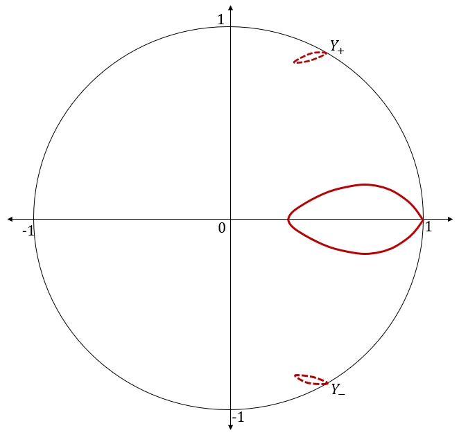
This is illustrated in Figure 3 for $\alpha=2$ , where the dashed curves in the upper-half plane and the lower-half plane, both oriented counterclockwise, correspond to $\theta\in(-c(\alpha),0)$ and $\theta\in(0,c(\alpha))$ , respectively.

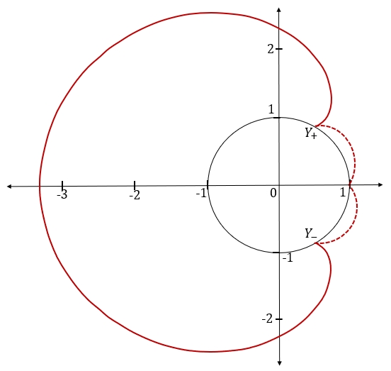
Next, observe that

\lim_{\theta\rightarrow c(\alpha)^{+}}y_{-}(e^{i\theta})=1=\lim_{\theta\rightarrow-c(\alpha)^{-}}y_{-}(e^{i\theta}),

and $\gamma_{J}$ can be identified as the path $\{(e^{i\theta},y_{-}(e^{i\theta}))\mid c(\alpha)<\theta<2\pi-c(\alpha)\}$ (with reversed orientation), implying

(3.2)

\partial\gamma_{J}=[[P_{2}^{+}]-[P_{2}^{-}]].

(For $\alpha=2$ , the $y$ -coordinate of this path is the bold curve inside the unit circle, as illustrated in Figure 3, oriented clockwise.) Define

\gamma_{J}^{\prime}=\left\{\left(\frac{1}{y_{-}\left(e^{i\theta}\right)},y_{-}\left(\frac{1}{y_{-}\left(e^{i\theta}\right)}\right)\right)\mid c(\alpha)<\theta<2\pi-c(\alpha)\right\}.

By some calculation, one sees that

	$\displaystyle y_{-}\left(\frac{1}{y_{-}\left(e^{i\theta}\right)}\right)$	$\displaystyle=e^{-i\theta},$
	$\displaystyle\lim_{\theta\rightarrow c(\alpha)^{+}}y_{-}(e^{i\theta})$	$\displaystyle=1=\lim_{\theta\rightarrow-c(\alpha)^{-}}y_{-}(e^{i\theta}),$

implying

(3.3)

\partial\gamma_{J}^{\prime}=[[P_{1}^{+}]-[P_{1}^{-}]].

Moreover, we have

	$\displaystyle\int_{\gamma_{J}}\eta(x,y)$	$\displaystyle=-\int_{c(\alpha)}^{2\pi-c(\alpha)}\log\|y_{+}\left(e^{i\theta}\right)\|\mathrm{d}\theta$
		$\displaystyle=\int_{c(\alpha)}^{2\pi-c(\alpha)}\log\|y_{-}\left(e^{i\theta}\right)\|\mathrm{d}\theta$
		$\displaystyle=\int_{c(\alpha)}^{2\pi-c(\alpha)}\log(\|1/y_{-}\left(e^{i\theta}\right)\|)\mathrm{d}(-\theta)$
		$\displaystyle=\int_{\gamma_{J}^{\prime}}\eta(x,y).$

Finally, we arrive at

\tilde{n}(\alpha)=I(\alpha)-2J(\alpha)=-\frac{1}{2\pi}\left(\int_{\gamma_{I}}\eta(x,y)-\int_{\gamma_{J}}\eta(x,y)-\int_{\gamma_{J}^{\prime}}\eta(x,y)\right)=-\frac{1}{2\pi}\int_{\tilde{\gamma}_{\alpha}}\eta(x,y),

where, by (3.1),(3.2), and (3.3), $\tilde{\gamma}_{\alpha}$ has trivial boundary, from which we can conclude that $\tilde{\gamma}_{\alpha}\in H_{1}(E_{\alpha},\mathbb{Z}).$ It is clear from the construction of the paths $\gamma_{I},\gamma_{J},$ and $\gamma_{J}^{\prime}$ that they are anti-invariant under the action of complex conjugation. Therefore, we have $\tilde{\gamma}_{\alpha}\in H_{1}(E_{\alpha},\mathbb{Z})^{-}$ , as desired. ∎

We shall use Theorem 8 and Lemma 9 to prove Theorem 2. We essentially follow an approach of Brunault [7] in identifying the path $\tilde{\gamma}_{2}$ as the push-forward of a path joining cusps on $X_{1}(19)$ with the aid of Magma and Pari/GP.

Proof of Theorem 2.

The elliptic curve $E_{2}:y^{2}+(x^{2}-2x)y+x=0$ has Cremona label $19a3$ , so it admits a modular parametrization $\varphi:X_{1}(19)\rightarrow E_{2}$ . Let $f_{2}$ be the weight $2$ newform of level $19$ associated to the curve $E_{2}$ and let $\omega=2\pi if_{2}(\tau)\mathrm{d}\tau,$ the pull-back of the holomorphic differential form on $E_{2}$ . Using Magma and Pari/GP codes in [7, §6.1], we find that

\int_{4/19}^{-4/19}\omega=-\Omega^{-}\approx-4.12709i,

where $\Omega^{-}$ is the imaginary period of $E_{2}$ obtained by subtracting twice the complex period from the real period of $E_{2}$ . Hence it follows that $\tilde{\gamma}_{2}=\varphi_{*}\left\{\frac{4}{19},-\frac{4}{19}\right\}$ , where $\tilde{\gamma}_{\alpha}$ is the path associated to $\tilde{n}(\alpha)$ . We have from [6, Tab. 1] that the curve $E_{2}$ can be parametrized by modular units, which are given explicitly as follows. Let

	$\displaystyle x(\tau)$	$\displaystyle=-\frac{g_{1}g_{7}g_{8}}{g_{2}g_{3}g_{5}},$
	$\displaystyle y(\tau)$	$\displaystyle=\frac{g_{1}g_{7}g_{8}}{g_{4}g_{6}g_{9}},$

where $g_{a}:=g_{a}(\tau)$ is as given in Theorem 8 with $N=19$ . By a result of Yang [24, Cor. 3], both $x(\tau)$ and $y(\tau)$ are modular functions on $\Gamma_{1}(19)$ . Multiplying each term by a modular form in $M_{2}(\Gamma_{1}(19))$ , one can apply Sturm’s theorem [22, Cor. 9.19], with the Sturm bound $B(M_{2}(\Gamma_{1}(19)))=60$ , to show that $y(\tau)^{2}+(x(\tau)^{2}-2x(\tau))y(\tau)+x(\tau)$ vanishes identically; i.e., $(x(\tau),y(\tau))$ parametrizes the curve $E_{2}$ . Finally, by Lemma 9 and Theorem 8, we find that

\tilde{n}(2)=-\frac{1}{2\pi}\int_{\tilde{\gamma}_{2}}\eta(x,y)=\frac{1}{2\pi}\int_{-4/19}^{4/19}\eta(x(\tau),y(\tau))=-\frac{1}{4\pi^{2}}L(57f_{2},2)=-3L^{\prime}(f_{2},0),

where the last equality follows from the functional equation for $L(f_{2},s)$ . ∎

In addition to (1.5), we discovered that, for all $\alpha\in(-1,3)$ which are cube roots of integers, the following identity holds numerically:

(3.4)

\tilde{n}(\alpha)\stackrel{{\scriptstyle?}}{{=}}r_{\alpha}L^{\prime}(E_{\alpha},0),

where $r_{\alpha}\in\mathbb{Q}$ . The data of $r_{\alpha}$ and $E_{\alpha}$ are given in Table 2.

$\alpha^{3}$	Cremona label of $E_{\alpha}$	$r_{\alpha}$	$\alpha^{3}$	Cremona label of $E_{\alpha}$	$r_{\alpha}$
$1$	$26a3$	$-1$	$14$	$2548d1$	$1/36$
$2$	$20a1$	$-5/3$	$15$	$1350i1$	$1/18$
$3$	$54a1$	$-2/3$	$16$	$44a1$	$-4/3$
$4$	$92a1$	$-1/3$	$17$	$2890e1$	$-1/27$
$5$	$550d1$	$-1/9$	$18$	$324b1$	$-1/6$
$6$	$756f1$	$-1/18$	$19$	$722a1$	$1/9$
$7$	$490a1$	$1/9$	$20$	$700i1$	$-1/9$
$8$	$19a3$	$-3$	$21$	$2464k1$	$-1/27$
$9$	$162c1$	$-1/3$	$22$	$2420d1$	$1/26$
$10$	$1700c1$	$1/36$	$23$	$1058b1$	$-1/12$
$11$	$242b1$	$-1/3$	$24$	$27a1$	$-3$
$12$	$540d1$	$1/9$	$25$	$50a1$	$-5/3$
$13$	$2366d1$	$-1/45$	$26$	$676c1$	$-1/6$

Table 2. Data for (3.4)

It might be possible to prove some formulas in this list by relating $\tilde{n}(\alpha)$ to known results in Table 1. In particular, the conjectural formulas for the curves of conductor $20,27,$ and $54$ are equivalent to the following identities:

	$\displaystyle\tilde{n}(\sqrt[3]{2})$	$\displaystyle\stackrel{{\scriptstyle?}}{{=}}-\frac{5}{8}n(\sqrt[3]{32}),$
	$\displaystyle\tilde{n}(\sqrt[3]{24})$	$\displaystyle\stackrel{{\scriptstyle?}}{{=}}-n(-6),$
	$\displaystyle\tilde{n}(\sqrt[3]{3})$	$\displaystyle\stackrel{{\scriptstyle?}}{{=}}-\frac{3}{2}n(-3).$

As a side note, the authors of [18] (incorrectly) proved

(3.5)

n(\sqrt[3]{2})=\frac{5}{6}L^{\prime}(E_{\sqrt[3]{2}},0)

(see the corollary under [18, Thm. 5]). In their arguments, they made use of the following functional identity for Mahler measures [13, Thm. 2.4]: for sufficiently small $|p|\neq 0$ ,

(3.6)

3g\left(\frac{1}{p}\right)=n\left(\frac{1+4p}{\sqrt[3]{p}}\right)+4n\left(\frac{1-2p}{\sqrt[3]{p^{2}}}\right),

where $g(\alpha)=\mathrm{m}((x+1)(y+1)(x+y)-\alpha xy)$ . When any of the arguments of $n$ in (3.6) enters the region inside the hypocycloid in Figure 1 (e.g. $p=-1/2$ in this case), this functional identity could be invalid due to discontinuity. Therefore, it is logically forbidden to deduce (3.5) from (3.6). In fact, by extending the hypergeometric formula (1.4) to the real line, Rogers [16] conjectured that

(3.7)

n(2)=\frac{3}{2}L^{\prime}(E_{2},0),

which is not the case by Theorem 2. It should be noted that both (3.5) and (3.7) make perfect sense if one thinks of $n(\alpha)$ as the right-hand side of $\eqref{E:naR}$ on the punctured real line. That said, this strange behavior of the function $n(\alpha)$ became a part of our motivation to initiate this project.

4. Final remarks

The family $Q_{\alpha}$ is among the several nonreciprocal families of two-variable polynomials studied by Boyd. Our results provide evidence of how Mahler measure behaves when the zero locus of a bivariate polynomial intersects the $2$ -torus nontrivially. This could shed some light on the discrepancies between Mahler measure and (elliptic) regulator, which is conjecturally related to $L$ -values under favorable conditions. Another family which possesses similar properties (i.e. nonreciprocality and temperedness) to $Q_{\alpha}$ is

S_{\alpha}=y^{2}+(x^{2}+\alpha x+1)y+x^{3},

which is labeled $(2\text{-}33)$ in [4]. Let $K$ be as defined in Section 1. Then for the family $S_{\alpha}$ we have $K\cap\mathbb{R}=[-4,2].$ For $\alpha$ in this range, the Mahler measure of $S_{\alpha}$ again splits naturally at the points of intersection between the curve $S_{\alpha}=0$ and the $2$ -torus. If $k=0$ , these points are $\pm i$ , and Boyd verified numerically that

(4.1)

\frac{1}{\pi}\int_{0}^{\pi/2}\log|y_{-}(e^{i\theta})|\mathrm{d}\theta-\frac{1}{\pi}\int_{\pi/2}^{\pi}\log|y_{-}(e^{i\theta})|\mathrm{d}\theta\stackrel{{\scriptstyle?}}{{=}}-L^{\prime}(E,0),

where $y_{-}(x)=-\frac{(x^{2}+1)}{2}\left(1-\sqrt{1-\frac{4x^{3}}{(x^{2}+1)^{2}}}\right)$ and $E$ is the conductor $11$ elliptic curve defined by $S_{0}=0$ . He also remarked

“This is in accord with our contention that in case $P$ vanishes on the torus, it is the integral of $\omega$ around a branch cut rather than $\mathrm{m}(P),$ which should be rationally related to $L^{\prime}(E,0)$ .”.

One might try to prove this identity using the investigation carried out in Section 3 and a result of Brunault [5] concerning Mahler measure of a conductor $11$ elliptic curve. We also discovered conjectural identities analogous to (4.1) for elliptic curves of conductor $17$ and $53$ , which are corresponding to $k=1$ and $k=-1$ , respectively. As opposed to the family $Q_{\alpha}$ , we are unable to find a general formula, both analytically and arithmetically, for Mahler measure (or its modification) of $S_{\alpha}$ , so the situation seems less apparent for this family.

We would also like to point out another related result in the literature which we find incomplete. In [10, Thm 3.1], Guillera and Rogers assert that for $q=e^{2\pi i\tau}\in(-1,1)$ if $\alpha=3\left(1+27\frac{\eta^{12}(3\tau)}{\eta^{12}(\tau)}\right)^{\frac{1}{3}},$ then

(4.2)

{n(\alpha)=\frac{9}{2\pi}\sum_{n=-\infty}^{\infty}D\left(e^{2\pi i/3}q^{n}\right)},

where $\eta(\tau)$ is the Dedekind eta function, and $D(z)$ is the Bloch-Wigner dilogarithm. The summation in the formula above can be seen as a value of the elliptic dilogarithm. Consider the curve $E_{2}$ , which appears in Theorem 2 and is isomorphic to $\mathbb{C}/\mathbb{Z}+\mathbb{Z}\tau$ , where $\tau=1/2+0.50586\ldots i.$ Then we have $q=e^{2\pi i\tau}=-0.04165\ldots$ . However, the identity (4.2) seems invalid in this case (and all other cases for $-1<\alpha<3)$ . The right-hand side is numerically equal to $\frac{3}{2}L^{\prime}(E_{2},0)$ , which is a conjecture of Bloch and Grayson [3], while $n(2)$ is not a rational multiple of $L^{\prime}(E_{2},0)$ . A correct formula for $\alpha\in(-1,3)$ should be

\tilde{n}(\alpha)=-\frac{9}{\pi}\displaystyle\sum_{n=-\infty}^{\infty}D\left(e^{2\pi i/3}q^{n}\right),

which can be proven using Lemma 9 and [7, Prop. 19].

Finally, we propose some problems for the interested readers.

(i)

The function $\tilde{n}(\alpha)$ looks somewhat unnatural at first glance. Is it possible to write it as the (full) Mahler measure of some polynomial?
(ii)

Do there exist algebraic integers $\beta$ for which $\sqrt[3]{\beta}\in(-1,3)$ and $\tilde{n}(\sqrt[3]{\beta})$ is a linear combination of $L^{\prime}(E,0)$ (i.e. identities analogous to (1.2))? As suggested by a result of Guillera and Rogers above, one might start by evaluating the function $u(\tau)=3\left(1+27\frac{\eta^{12}(3\tau)}{\eta^{12}(\tau)}\right)^{\frac{1}{3}}$ at some suitable CM points and numerically compare $\tilde{n}(u(\tau))$ with related elliptic $L$ -values using the PSLQ algorithm.

Funding

This work was supported by the National Research Council of Thailand (NRCT) under the Research Grant for Mid-Career Scholar [N41A640153 to D.S.].

Acknowledgements

The author is indebted to Wadim Zudilin for helpful discussions and his suggestion about integral and hypergeometric identities in the proofs of Lemma 6 and Lemma 7. The author would also like to thank François Brunault for his guidance on an approach to proving Lemma 9 and his explanation about Deninger’s results. This work would not have been complete without insightful comments from Mat Rogers and François Brunault on early versions of this manuscript, so the author would like to acknowledge them here. Finally, the author thanks Yusuke Nemoto and Zhengyu Tao for bringing a sign error in Theorem 1 and a miscalculation in the proof of Lemma 9 in the previous version of this paper to his attention.

References

[1] George E. Andrews, Richard Askey, and Ranjan Roy, Special functions, Encyclopedia of Mathematics and its Applications, vol. 71, Cambridge University Press, Cambridge, 1999. MR 1688958
[2] Bruce C. Berndt, Ramanujan’s notebooks. Part V, Springer-Verlag, New York, 1998. MR 1486573
[3] S. Bloch and D. Grayson, $K_{2}$ and $L$ -functions of elliptic curves: computer calculations, Applications of algebraic $K$ -theory to algebraic geometry and number theory, Part I, II (Boulder, Colo., 1983), Contemp. Math., vol. 55, Amer. Math. Soc., Providence, RI, 1986, pp. 79–88. MR 862631
[4] David W. Boyd, Mahler’s measure and special values of $L$ -functions, Experiment. Math. 7 (1998), no. 1, 37–82. MR 1618282
[5] François Brunault, Version explicite du théorème de Beilinson pour la courbe modulaire $X_{1}(N)$ , C. R. Math. Acad. Sci. Paris 343 (2006), no. 8, 505–510. MR 2267584
[6] by same author, Parametrizing elliptic curves by modular units, J. Aust. Math. Soc. 100 (2016), no. 1, 33–41. MR 3436769
[7] by same author, Regulators of Siegel units and applications, J. Number Theory 163 (2016), 542–569. MR 3459587
[8] Christopher Deninger, Deligne periods of mixed motives, $K$ -theory and the entropy of certain ${\bf Z}^{n}$ -actions, J. Amer. Math. Soc. 10 (1997), no. 2, 259–281. MR 1415320
[9] NIST Digital Library of Mathematical Functions, http://dlmf.nist.gov/, Release 1.0.23 of 2019-06-15, F. W. J. Olver, A. B. Olde Daalhuis, D. W. Lozier, B. I. Schneider, R. F. Boisvert, C. W. Clark, B. R. Miller and B. V. Saunders, eds.
[10] Jesús Guillera and Mathew Rogers, Mahler measure and the WZ algorithm, Proc. Amer. Math. Soc. 143 (2015), no. 7, 2873–2886. MR 3336612
[11] Leon M. Hall, Missouri S&T Math 483, Lecture Notes: Special Functions.
[12] Matilde Lalín, Detchat Samart, and Wadim Zudilin, Further explorations of Boyd’s conjectures and a conductor 21 elliptic curve, J. Lond. Math. Soc. (2) 93 (2016), no. 2, 341–360. MR 3483117
[13] Matilde N. Lalin and Mathew D. Rogers, Functional equations for Mahler measures of genus-one curves, Algebra Number Theory 1 (2007), no. 1, 87–117. MR 2336636
[14] Yotsanan Meemark and Detchat Samart, Mahler measures of a family of non-tempered polynomials and Boyd’s conjectures, Res. Math. Sci. 7 (2020), no. 1, Paper No. 1, 20. MR 4042306
[15] Anton Mellit, Elliptic dilogarithms and parallel lines, J. Number Theory 204 (2019), 1–24. MR 3991411
[16] Mathew Rogers, personal communication, 2010.
[17] by same author, Hypergeometric formulas for lattice sums and Mahler measures, Int. Math. Res. Not. IMRN (2011), no. 17, 4027–4058. MR 2836402
[18] Mathew Rogers and Wadim Zudilin, From $L$ -series of elliptic curves to Mahler measures, Compos. Math. 148 (2012), no. 2, 385–414. MR 2904192
[19] Detchat Samart, Mahler measures as linear combinations of $L$ -values of multiple modular forms, Canad. J. Math. 67 (2015), no. 2, 424–449. MR 3314841
[20] A. Schinzel, Polynomials with special regard to reducibility, Encyclopedia of Mathematics and its Applications, vol. 77, Cambridge University Press, Cambridge, 2000, With an appendix by Umberto Zannier. MR 1770638
[21] C. J. Smyth, On measures of polynomials in several variables, Bull. Austral. Math. Soc. 23 (1981), no. 1, 49–63. MR 615132
[22] William Stein, Modular forms, a computational approach, Graduate Studies in Mathematics, vol. 79, American Mathematical Society, Providence, RI, 2007, With an appendix by Paul E. Gunnells. MR 2289048
[23] F. Rodriguez Villegas, Modular Mahler measures. I, Topics in number theory (University Park, PA, 1997), Math. Appl., vol. 467, Kluwer Acad. Publ., Dordrecht, 1999, pp. 17–48. MR 1691309
[24] Yifan Yang, Transformation formulas for generalized Dedekind eta functions, Bull. London Math. Soc. 36 (2004), no. 5, 671–682. MR 2070444
[25] Wadim Zudilin, Regulator of modular units and Mahler measures, Math. Proc. Cambridge Philos. Soc. 156 (2014), no. 2, 313–326. MR 3177872

	$\displaystyle-\frac{2\lambda}{\lambda^{3}+4}{}_{2}F_{1}\biggl{(}\genfrac{.}{.}{0.0pt}{}{\frac{1}{3}\mathchar 44\relax\mkern 6.0mu\frac{2}{3}}{1}\,\,\bigg{\|}\,\,\frac{27\lambda^{6}}{(\lambda^{3}+4)^{3}}\biggr{)}$	$\displaystyle=-\frac{\sqrt[3]{4(p+p^{2})}}{2(p^{2}+p+1)}{}_{2}F_{1}\biggl{(}\genfrac{.}{.}{0.0pt}{}{\frac{1}{3}\mathchar 44\relax\mkern 6.0mu\frac{2}{3}}{1}\,\,\bigg{\|}\,\,\frac{27p^{2}(1+p)^{2}}{4(1+p+p^{2})^{3}}\biggr{)}$
		$\displaystyle=-\frac{\sqrt[3]{4(p+p^{2})}}{2\sqrt{1+2p}}{}_{2}F_{1}\biggl{(}\genfrac{.}{.}{0.0pt}{}{\frac{1}{2}\mathchar 44\relax\mkern 6.0mu\frac{1}{2}}{1}\,\,\bigg{\|}\,\,\frac{p^{3}(2+p)}{1+2p}\biggr{)}$
		$\displaystyle=-\frac{\lambda}{2\sqrt[4]{\lambda^{3}+1}}{}_{2}F_{1}\biggl{(}\genfrac{.}{.}{0.0pt}{}{\frac{1}{2}\mathchar 44\relax\mkern 6.0mu\frac{1}{2}}{1}\,\,\bigg{\|}\,\,\rho(\lambda)\biggr{)},$

	$\displaystyle\int_{\gamma_{J}}\eta(x,y)$	$\displaystyle=-\int_{c(\alpha)}^{2\pi-c(\alpha)}\log\|y_{+}\left(e^{i\theta}\right)\|\mathrm{d}\theta$
		$\displaystyle=\int_{c(\alpha)}^{2\pi-c(\alpha)}\log\|y_{-}\left(e^{i\theta}\right)\|\mathrm{d}\theta$
		$\displaystyle=\int_{c(\alpha)}^{2\pi-c(\alpha)}\log(\|1/y_{-}\left(e^{i\theta}\right)\|)\mathrm{d}(-\theta)$
		$\displaystyle=\int_{\gamma_{J}^{\prime}}\eta(x,y).$

Mahler measure of a nonreciprocal family of elliptic curves

Abstract.

1. Introduction

Theorem 1.

Theorem 2.

2. The hypergeometric formula

Lemma 3.

Proof.

Proposition 4.

Proof.

Lemma 5.

Proof.

Lemma 6.

Proof.

Lemma 7.

Proof.

Proof of Theorem 1.

3. Relation to elliptic regulators and LL-values

Theorem 8 (Brunault-Mellit-Zudilin).

Lemma 9.

Proof.

Proof of Theorem 2.

4. Final remarks

Funding

Acknowledgements

References

3. Relation to elliptic regulators and $L$ -values