Magnetization oscillations in a periodically driven transverse field Ising chain

Introduction.—Time-dependent quantum systems have attracted continuous attention in the past few decades, leading to rich experimental and theoretical progress. These include time crystals [1, 2, 3, 4], nonlinear electron spin resonance and photon-induced phase transitions [5, 6, 7, 8, 9, 10], measurement induced exotic phenomena [11, 12, 13, 14, 15], as well as Kibble-Zurek mechanism [16, 17, 18, 19, 20]. Along the course the transverse-field quantum Ising chain (TFIC) serves as a prototypical system for investigating out of equilibrium dynamics [21, 22, 23]. For a static transverse field, the system is one of the simplest solvable models that accommodates quantum phase transition [24, 25]. At its quantum critical point (QCP), the system exhibits conformal invariance [26]. Introducing a perturbation field along the Ising-spin direction at the QCP gives rise, in the scaling limit, to an integrable field theory known as quantum $E_{8}$ integrable model [27, 28, 29, 30, 31, 32, 33, 34]. When the transverse field is time dependent, a complete analytical understanding poses a significant challenge.

There are two different widely-studied forms of the time-dependent magnetic field. One is a sudden change of the magnetic field at the initial time [35, 21, 36, 37, 38, 39], and the other is a periodically driven magnetic field [40, 10, 41]. For a sudden quench involving a nonzero longitudinal field, the dynamics of both the one-point functions and the entanglement entropy reveal fingerprints of the confinement phenomenon [36, 37, 38, 42, 43, 44, 45, 46]. For the periodic driving, it has been proved that for a rotating field in the transverse plane, the time evolution can be related to the TFIC with the presence of an effective longitudinal field proportional to the rotation frequency [41, 40].

In this letter, we focus on the critical Ising chain with a periodically driven magnetic field that slowly rotates in the transverse plane. Under a rotational wave transformation [47], the time evolution process can be effectively related to a time-independent critical TFIC perturbed by an effective longitudinal field proportional to the rotation frequency [40]. In the scaling limit, the effective model becomes the quantum $E_{8}$ integrable model [31]. Using the exact form factors of the model and the post-quench perturbative framework [28, 48, 42, 17, 31, 49, 50, 38], we analytically determine the time evolution of the magnetization components $M^{\alpha}$ $(\alpha=x,y,z)$ in both the time and frequency domains, where the dominant low-energy spectrum can be understood through contributions from different particle states of the quantum $E_{8}$ integrable model.

For the magnetization spectra $M^{z}(\omega)$, we find that the low-energy collective excitations in frequency domain are dominated by cascades of singular peaks of two different types: the $\delta$-function type and the edge-singularity type. The former singular peaks are contributed by the particle excitations of an $E_{8}$ particle with either the vacuum or a different particle. The latter are due to the particle excitations of two particles with either the vacuum or an $E_{8}$ particle, or due to the particle excitations of two sets of two particles, where the two sets contain particles of the same type  [51]. For the magnetization spectra $M^{x}(\omega)$ and $M^{y}(\omega)$, cascades of singular peaks also appear with similar structure and the same origin, but split into two sets with respect to the peaks of $M^{z}(\omega)$, with their corresponding frequency shifts matching the rotating frequency of the transverse field. Numerical verification using the infinite time-evolving block decimation (iTEBD) algorithm is also presented, supporting the analytical results. Finally, a Rydberg-atom quantum simulator is proposed for future experimental study, providing a promising way to simulate and investigate the interplay of non-equilibrium physics and quantum integrability.

Model.—The Hamiltonian of a critical Ising chain subjected to a periodically driven transverse field $\vec{B}(t)=({\cos(\omega_{0}t)}$, $-\sin(\omega_{0}t),0)$ is given by

where $\sigma_{i}^{\alpha}(\alpha=x,~{}y,~{}z)$ represent the Pauli matrices at site $i$, and we assume that the rotation frequency $(\hbar)\omega_{0}\ll J$. Hereafter, $\hbar$ and $J$ are set as 1. At $t=0$, the system is a critical TFIC, and we set the initial state to be its ground state. By using a unitary transformation [41, 40, 16, 51],

the time-evolved wave function $|\psi(t)\rangle$ is given by

with the effective static Hamiltonian

which is a quantum critical TFIC perturbed by an effective longitudinal field $\omega_{0}/2$. We consider the time-dependent magnetization along the $x$, $y$, and $z$ directions,

Introducing the time-dependent magnetic components $D^{\alpha}(t)$ as

the time-dependent magnetization $M^{\alpha}(t)$ components are

It is in general difficult to determine Eq. (6) analytically. However, for small $\omega_{0}$ the effective Hamiltonian Eq. (4) turns out to be the quantum $E_{8}$ Hamiltonian in the scaling limit [27, 28, 31],

Here, $\mathcal{H}_{c=1/2}$ represents the Hamiltonian of conformal field theory (CFT) with central charge $c=1/2$. The coupling intensity $h$ corresponds to $\omega_{0}/2$ in the scaling limit. The Pauli matrices $\sigma^{z}$ and $\sigma^{x}$ correspond to the primary fields of the Ising and energy density fields $\sigma$ and $\varepsilon$, respectively. In the quantum $E_{8}$ integrable model, the matrix elements of these two primary fields can be determined using the form factor bootstrap method [28, 42, 31, 51]. Taking the scaling limit of $D^{\alpha}(t)$ [Eq. (6)]

for $\mathcal{O}=\varepsilon,\sigma$, hereafter the math script font of corresponding physical quantity refers to the scaling limit. We have inserted two complete $E_{8}$ bases $\{|n;j\rangle\}$ and $\{|m;k\rangle\}$ where we organize the states according to their particle numbers $n$ and $m$ and $j,k$ label states within these sectors. Then $A^{\mathcal{O}}_{nm}(t)=\sum_{j,k}e^{i(E_{n;j}-E_{m;k})t}\langle\psi_{s}(0)|n;j\rangle\langle n;j|\mathcal{O}|m;k\rangle\langle m;k|\psi_{s}(0)\rangle$, with $|\psi_{s}(0)\rangle$ being $|\psi(0)\rangle$ in the scaling limit. In addition, $E_{n;j}$ and $E_{m;k}$ are eigenenergies of the two $E_{8}$ eigenstates $|n;j\rangle$ and $|m;k\rangle$, respectively. The overlaps $\langle m;k|\psi_{s}(0)\rangle$ can be determined using a post-quench perturbative framework [38, 42, 17, 51], and the explicit form of the $A^{\mathcal{O}}_{nm}(t)$ can be found in [51]. In the following, we call the terms in Eq. (9) with fixed particle numbers particle channels. The remaining challenge is to determine $D^{y}(t)$ in the scaling limit, as $\sigma^{y}$ does not correspond to a primary field in the Ising CFT. However, starting from the lattice formalism, we notice [52, 31, 51]

Therefore, by taking the system back to the scaling limit we can simultaneously determine $\mathscr{D}^{\sigma}$ and $\mathscr{D}^{y}$.

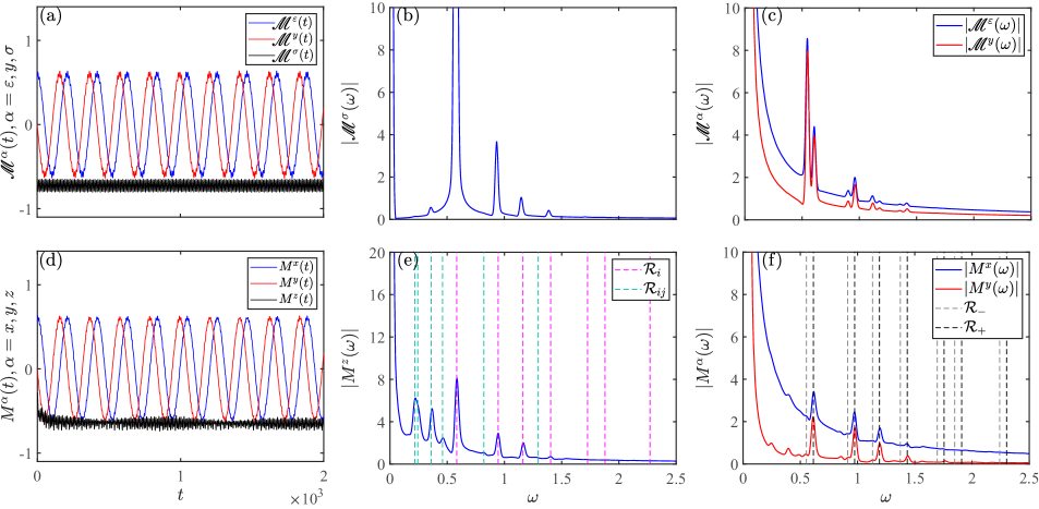
Singular peaks.—Using Eq. (7) and Eq. (10), the results for $\mathscr{M}^{\mathcal{O}}(t)$, with $\mathcal{O}=\varepsilon,y$, and $\sigma$, are displayed in Fig. 1 (a), after normalization with $m_{1}=C_{\omega}{\omega_{0}}^{8/15}$, $\langle\sigma\rangle=-C_{\sigma}{\omega_{0}}^{1/15}$ and $\langle\varepsilon\rangle=\langle\varepsilon\rangle_{h=0}-C_{\varepsilon}{\omega_{0}}^{8/15}$. Here we set $\omega_{0}=0.03$, and the explicit values of $C_{\omega}$, $C_{\sigma}$ and $C_{\varepsilon}$ can be found in [51]. To better understand the collective excitations in the time-dependent magnetization, we consider magnetization in the frequency domain following the one-sided Fourier transformation,

We present our analytical results alongside those obtained from numerical iTEBD simulations in Figure 1. To facilitate a clearer comparison between the analytical and numerical outcomes, we applied Gaussian broadening with a broadening factor of $\alpha=2\%$. The detailed analytical expressions are provided in [51]. As can be seen in the figure, the dominant singular peaks predicted by the analytical field-theoretical approach are verified by the numerical simulations, which, overall, are given by contributions from single- and two-$E_{8}$-particle channels in the frequency domain [42, 51]. For $\mathscr{M}^{\sigma}(\omega)$ [$M^{z}(\omega)$ for the lattice simulation], cascades of singular peaks $\{\mathcal{R}\}$ are found in the low-energy excitations. Such singular peaks are corresponding to two different types of singular behaviors: the $\delta$-function type and the edge-singularity type. For the $\delta$-function peaks, besides those peaks from an $E_{8}$ particle and the $E_{8}$ vacuum, other peaks emerge from the contributions of two different $E_{8}$ particles, with the corresponding frequency being their mass difference [36, 38, 49, 51]. For the edge-singularity peaks, they have two distinct origins. The first one is due to the divergence in the density of states of $E_{8}$ particles, also known as Van Hove singularity [31, 53]. Such edge-singularity peaks are contributed by two different $E_{8}$ particles $m_{i},~{}m_{j}$, and the other one being either the $E_{8}$ vacuum or a different $E_{8}$ particle $m_{k}$, showing a singular behavior as $1/\sqrt{\omega-\omega_{\text{th}}}$, where $\omega_{\text{th}}=m_{i}+m_{j}$ (or $=m_{i}+m_{j}-m_{k}$) being the threshold [51]. The second one originates from the kinematic singularities of the multi-particle form factor of the quantum $E_{8}$ field theory [51, 28, 42, 31, 53], associated with the particle channels of two distinct sets of $E_{8}$ particles. One set comprises two $E_{8}$ particles $m_{i}$ and $m_{k}$, while the other set includes two $E_{8}$ particles with at least one of the same type as $m_{j}$ and $m_{k}$. These contribute $\ln(\omega+m_{i}-m_{j})$ edge-singularities in addition to the previous $\delta$-function peaks at the thresholds of $\omega_{\text{th}}=m_{j}-m_{i}$. It is worth noticing that in the particle channels of a single to two $E_{8}$ particles, the kinematic poles also appear and seem to contribute additional singularities, which will eventually be cancelled due to the exchange property of the multi-particle form factors  [51]. In the numerical simulation of the Hamiltonian Eq. (1), by comparing the corresponding frequencies of the peaks with the analytical predictions, the dominant contributions are identified as $\delta$-function peaks [dashed vertical lines in Fig. 1 (e)], with their detailed frequencies listed in Table. 1. Additionally, other singularity peaks are identified as edge-singularity peaks contributed by the vacuum-to-two-particle channels of $m_{1}m_{2}$, the one-to-two-particle channels of $m_{5}-m_{1}m_{4}$ and $m_{1}m_{2}-m_{5}$ [51]. However, for the later two classes, the heavy $E_{8}$-particle channels are not shown in the analytical results due to the high computational cost of form factor calculations.

In the spectra of $\mathscr{M}^{\varepsilon}(\omega)$ and $\mathscr{M}^{y}(\omega)$, the stable singular peaks $\{\mathcal{R}\}$ are further separated into two distinct groups of new singular peaks $\{\mathcal{R}^{\pm}\}$, where the corresponding excitation frequencies have been shifted as $m_{\mathcal{R}}\pm\omega_{0}$, shown in Fig. 1 (c). This special feature is also captured by the numerical simulation for $M^{x}(\omega)$ and $M^{y}(\omega)$ [Fig. 1 (f)], where the separated single $E_{8}$ particles are also highlighted by dashed vertical lines. The numerical verification agrees well with the analytical results.

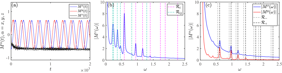
Implementation in a Rydberg qubit array.— For possible experimental study of the $E_{8}$ physics in a periodically driven system, we propose a many-body time-dependent Rydberg Hamiltonian [54, 55],

where $|r_{i}\rangle=|1_{i}\rangle$ and $|g_{i}\rangle=|0_{i}\rangle$ are the representation of the Rydberg states and the ground states on the $i^{th}$ qubit, respectively. The amplitude and phase of the driving laser field is $\Omega(t)$ and $\phi(t)$, respectively. The operator $n_{i}=|r_{i}\rangle\langle r_{i}|$ counts the Rydberg excitations, and $x_{i}=ia$ are the coordinate for the $i$-th qubit with $a$ being the lattice spacing. $\Omega(t)$, $\phi(t)$, $\Delta(t)$ and $C_{6}$ are the corresponding (time-dependent) coefficients, whose values can be found in Ref. [54]. By applying a transformation between the Rydberg states and an effective Ising basis $\sigma_{i}^{+}=|g_{i}\rangle\langle r_{i}|,~{}\sigma_{i}^{-}=|r_{i}\rangle\langle g_{i}|,~{}\sigma_{i}^{z}=\mathbf{1}-2n_{i}$, this Rydberg Hamiltonian can be transformed to a periodically driven transverse field Ising chain. Since the interaction strength decays as $1/|i-j|^{6}$, we neglect spin interaction term with distance larger than 2 lattice sites, so the effective Hamiltonian follows [55],

where $\lambda=1/2^{6}$. Using iTEBD algorithm, we find that the model hosts a quantum phase transition at the quantum critical point $g_{c}=1.0275$, which also falls into the TFIC universality class. The rotating frequency is set as $\omega_{0}=0.03$. All the corresponding numerical results are shown in Fig. 2 (a), (b) and (c), with a Gaussian broadening $\alpha=2\%$. The dominated low-energy physics proposed by the quantum $E_{8}$ integrable field theory are well captured by the numerical lattice simulation results, and the corresponding peaks are also shown in Table. 1. It can be found that the additional next nearest neighboring Ising interaction only slightly modifies the frequency of the singular peaks. Our numerical simulations on Eq. (13) implies that the $E_{8}$ physics revealed in the time-dependent model [Eq. (1)] is fully accessible through a practical Rydberg qubit array experimental setup.

Conclusions.—In this letter, we showed that the time evolution of the magnetization in the Ising chain under a slowly rotating transverse field can be described via the integrable $E_{8}$ quantum field theory and its particle content. Based on a post-quench perturbation framework, along with the $E_{8}$ form factor theory, we analytically determined the magnetizations in both the time and frequency domains. Along the $z$ direction, we identified two types of singular peaks in the frequency domain: the $\delta$-function and the edge-singularity types. The frequencies of the $\delta$-function peaks are given by the masses and mass differences of $E_{8}$ particles. The edge-singularity peaks are essentially the Van Hove singularities given by the divergence of the density of states, or the kinematic singularities of the multi-particle $E_{8}$ form factors. A significant contribution given by the particle combination $m_{1}m_{2}$ is found in the numerical data. Moreover, for the magnetizations along the $x$ and $y$ directions, in the frequency domain all the singular peaks are split into two sets of new peaks with their corresponding frequency shifts matching the rotation frequency.

For a possible experimental implementation, we proposed a neutral atom Rydberg quantum simulator that can realize a modified periodically driven transverse field Ising chain. We confirmed numerically that despite the possible presence of next-nearest-neighbor couplings, it can realize the expected magnetization spectra, thus providing a novel and practical route to access the quantum $E_{8}$ physics in a time-dependent system.

Switching on a static transverse field provides an exciting opportunity to study the dynamics of confinement, which we leave for future work. Our work may also inspire further studies of non-equilibrium physics via quantum integrability.

Acknowledgements.—We thank Ning Xi, Zongping Gong and Zilong Li for discussions, Congjun Wu for helpful discussion during an early stage of the work. The work at Shanghai Jiao Tong University is sponsored by National Natural Science Foundation of China No. 12274288 and the Innovation Program for Quantum Science and Technology Grant No. 2021ZD0301900. MK was supported by the National Research, Development and Innovation Office of Hungary (NKFIH) through the OTKA Grant K138606. The work of M.O. was partially supported by the JSPS KAKENHI Grants No. JP23K25791 and No. JP24H00946.

References

- Wilczek [2012] F. Wilczek, Phys. Rev. Lett. 109, 160401 (2012).
- Shapere and Wilczek [2012] A. Shapere and F. Wilczek, Phys. Rev. Lett. 109, 160402 (2012).
- Watanabe and Oshikawa [2015] H. Watanabe and M. Oshikawa, Phys. Rev. Lett. 114, 251603 (2015).
- Yang and Cai [2021] X. Yang and Z. Cai, Phys. Rev. Lett. 126, 020602 (2021).
- Oshikawa and Affleck [1999] M. Oshikawa and I. Affleck, Phys. Rev. Lett. 82, 5136 (1999).
- Oshikawa and Affleck [2002] M. Oshikawa and I. Affleck, Phys. Rev. B 65, 134410 (2002).
- Iwai et al. [2003] S. Iwai, M. Ono, A. Maeda, H. Matsuzaki, H. Kishida, H. Okamoto, and Y. Tokura, Phys. Rev. Lett. 91, 057401 (2003).
- Okamoto et al. [2011] H. Okamoto, T. Miyagoe, K. Kobayashi, H. Uemura, H. Nishioka, H. Matsuzaki, A. Sawa, and Y. Tokura, Phys. Rev. B 83, 125102 (2011).
- Kitagawa et al. [2011] T. Kitagawa, T. Oka, A. Brataas, L. Fu, and E. Demler, Phys. Rev. B 84, 235108 (2011).
- Oka and Aoki [2009] T. Oka and H. Aoki, Phys. Rev. B 79, 081406 (2009).
- Skinner et al. [2019] B. Skinner, J. Ruhman, and A. Nahum, Phys. Rev. X 9, 031009 (2019).
- Tang and Zhu [2020] Q. Tang and W. Zhu, Phys. Rev. Res. 2, 013022 (2020).
- Yang et al. [2023a] Z. Yang, D. Mao, and C.-M. Jian, Phys. Rev. B 108, 165120 (2023a).
- Lee et al. [2023] J. Y. Lee, C.-M. Jian, and C. Xu, PRX Quantum 4, 030317 (2023).
- Ashida et al. [2023] Y. Ashida, S. Furukawa, and M. Oshikawa, arXiv:2311.16343 (2023).
- Quan and Zurek [2010] H. T. Quan and W. H. Zurek, New Journal of Physics , 093025 (2010).
- Hódsági and Kormos [2020] K. Hódsági and M. Kormos, SciPost Phys. 9, 055 (2020).
- Jamadagni et al. [2024] A. Jamadagni, J. Kazemi, and A. Bhattacharyya, Phys. Rev. B 110, 045140 (2024).
- Allman et al. [2024] D. G. Allman, P. Sabharwal, and K. C. Wright, Phys. Rev. A 109, 053320 (2024).
- Bayocboc et al. [2024] F. A. Bayocboc, J. Dziarmaga, and W. H. Zurek, Phys. Rev. B 109, 064501 (2024).
- Calabrese et al. [2011] P. Calabrese, F. H. L. Essler, and M. Fagotti, Phys. Rev. Lett. 106, 227203 (2011).
- Calabrese et al. [2012a] P. Calabrese, F. H. L. Essler, and M. Fagotti, J. Stat. Mech. 2012, P07016 (2012a).
- Calabrese et al. [2012b] P. Calabrese, F. H. L. Essler, and M. Fagotti, J. Stat. Mech. 2012, P07022 (2012b).
- Pfeuty [1970] P. Pfeuty, Ann. Phys. 59, 79 (1970).
- Sachdev [2011] S. Sachdev, Quantum Phase Transitions (Cambridge University Press, Cambridge, England, 2011) pp. 1–521.
- Boyanovsky [1989] D. Boyanovsky, Phys. Rev. B 39, 6744 (1989).
- Zamolodchikov [1989] A. B. Zamolodchikov, Int. J. Mod. Phys. A 04, 4235 (1989).
- Delfino and Mussardo [1995] G. Delfino and G. Mussardo, Nucl. Phys. B 455, 724 (1995).
- Zhang et al. [2020] Z. Zhang, K. Amelin, X. Wang, H. Zou, J. Yang, U. Nagel, T. Rõõm, T. Dey, A. A. Nugroho, T. Lorenz, J. Wu, and Z. Wang, Phys. Rev. B 101, 220411 (2020).
- Zou et al. [2021] H. Zou, Y. Cui, X. Wang, Z. Zhang, J. Yang, G. Xu, A. Okutani, M. Hagiwara, M. Matsuda, G. Wang, G. Mussardo, K. Hódsági, M. Kormos, Z. He, S. Kimura, R. Yu, W. Yu, J. Ma, and J. Wu, Phys. Rev. Lett. 127, 077201 (2021).
- Wang et al. [2021a] X. Wang, H. Zou, K. Hódsági, M. Kormos, G. Takács, and J. Wu, Phys. Rev. B 103, 235117 (2021a).
- Yang et al. [2023b] J. Yang, X. Wang, and J. Wu, J. Phys A: Math. Theor. 56, 013001 (2023b).
- Wang et al. [2021b] X. Wang, J. Yang, and J. Wu, Acta Phys. Sin. 70, 230504 (2021b).
- Wang et al. [2023] X. Wang, K. Puzniak, K. Schmalzl, C. Balz, M. Matsuda, A. Okutani, M. Hagiwara, J. Ma, J. Wu, and L. Bella, arXiv:2308.00249 (2023).
- Caux and Essler [2013] J.-S. Caux and F. H. L. Essler, Phys. Rev. Lett. 110, 257203 (2013).
- Kormos et al. [2017] M. Kormos, M. Collura, G. Takács, and P. Calabrese, Nat. Phys. 13, 246 (2017).
- Delfino and Viti [2017] G. Delfino and J. Viti, J. Phys A: Math. Theor. 50, 084004 (2017).
- Hódsági et al. [2018] K. Hódsági, M. Kormos, and G. Takács, SciPost Phys. 5, 027 (2018).
- Granet et al. [2020] E. Granet, M. Fagotti, and F. H. L. Essler, SciPost Phys. 9, 033 (2020).
- Robinson et al. [2021] N. J. Robinson, I. P. Castillo, and E. Guzmán-González, Phys. Rev. B 103, L140407 (2021).
- Takayoshi et al. [2014] S. Takayoshi, H. Aoki, and T. Oka, Phys. Rev. B 90, 085150 (2014).
- Hódsági et al. [2019] K. Hódsági, M. Kormos, and G. Takács, J. High Energy Phys. 2019 (8).
- Lerose et al. [2020] A. Lerose, F. M. Surace, P. P. Mazza, G. Perfetto, M. Collura, and A. Gambassi, Phys. Rev. B 102, 041118 (2020).
- Vovrosh and Knolle [2021] J. Vovrosh and J. Knolle, Sci. Rep. 11, 11577 (2021).
- Birnkammer et al. [2022] S. Birnkammer, A. Bastianello, and M. Knap, Nat. Commun. 13, 7663 (2022).
- Krasznai and Takács [2024] A. Krasznai and G. Takács, SciPost Phys. 16, 138 (2024).
- Wu and Yang [2007] Y. Wu and X. Yang, Phys. Rev. Lett. 98, 013601 (2007).
- Kormos and Takács [2010] M. Kormos and G. Takács, J. High Energy Phys. 2010 (112).
- Castro-Alvaredo et al. [2020] O. A. Castro-Alvaredo, M. Lencsés, I. M. Szécsényi, and J. Viti, Phys. Rev. Lett. 124, 230601 (2020).
- Castro-Alvaredo et al. [2019] O. A. Castro-Alvaredo, M. Lencsés, I. M. Szécsényi, and J. Viti, J. High Energy Phys. 2019 (79).
- [51] See Supplemental Material at [URL will be inserted by publisher]. For details of the form factors used in the main text, details of the analytical results of the main text, a discussion of connecting the lattice and field theory results and a detailed discussion of the singularity behaviours.
- Wu et al. [2014] J. Wu, M. Kormos, and Q. Si, Phys. Rev. Lett. 113, 247201 (2014).
- Cubero et al. [2022] A. C. Cubero, R. M. Konik, M. Lencsés, G. Mussardo, and G. Takács, SciPost Phys. 12, 162 (2022).
- Wurtz et al. [2023] J. Wurtz, A. Bylinskii, B. Braverman, J. Amato-Grill, S. H. Cantu, F. Huber, A. Lukin, F. Liu, P. Weinberg, J. Long, S.-T. Wang, N. Gemelke, and A. Keesling, arXiv:2306.11727 (2023).
- Monroe et al. [2021] C. Monroe, W. C. Campbell, L.-M. Duan, Z.-X. Gong, A. V. Gorshkov, P. W. Hess, R. Islam, K. Kim, N. M. Linke, G. Pagano, P. Richerme, C. Senko, and N. Y. Yao, Rev. Mod. Phys. 93, 025001 (2021).
- Fateev [1994] V. Fateev, Phys. Lett. B 324, 45 (1994).
- Wu et al. [2018] J. Wu, L. Zhu, and Q. Si, Phys. Rev. B 97, 245127 (2018).
Appendix A Supplemental Material—Magnetization oscillations in a periodically driven transverse field Ising chain
Appendix B A. The emergent quantum integrable model
In this appendix, we review the derivation of the effective static Hamiltonian and its scaling limit originally given in Ref. [40]. We start from the original periodically driven transverse field Ising chain to derive the emergent quantum model. The Schrdinger equation is