Magnetic reconnection between loops accelerated by a nearby filament eruption
Abstract
Magnetic reconnection modulated by non-local disturbances in the solar atmosphere has been investigated theoretically, but rarely observed. In this study, employing H and extreme ultraviolet (EUV) images and line of sight magnetograms, we report acceleration of reconnection by adjacent filament eruption. In H images, four groups of chromospheric fibrils are observed to form a saddle-like structure. Among them, two groups of fibrils converge and reconnect. Two newly reconnected fibrils then form, and retract away from the reconnection region. In EUV images, similar structures and evolution of coronal loops are identified. Current sheet forms repeatedly at the interface of reconnecting loops, with width and length of 1-2 and 5.3-7.2 Mm, and reconnection rate of 0.18-0.3. It appears in the EUV low-temperature channels, with average differential emission measure (DEM) weighed temperature and EM of 2 MK and 2.51027 cm-5. Plasmoids appear in the current sheet and propagate along it, and then further along the reconnection loops. The filament, located at the southeast of reconnection region, erupts, and pushes away the loops covering the reconnection region. Thereafter, the current sheet has width and length of 2 and 3.5 Mm, and reconnection rate of 0.57. It becomes much brighter, and appears in the EUV high-temperature channels, with average DEM-weighed temperature and EM of 5.5 MK and 1.71028 cm-5. In the current sheet, more hotter plasmoids form. More thermal and kinetic energy is hence converted. These results suggest that the reconnection is significantly accelerated by the propagating disturbance caused by the nearby filament eruption.
1 Introduction
As the reconfiguration of magnetic field geometry, magnetic reconnection plays an elemental role in magnetized plasma systems, e.g., the solar and stellar coronae and planetary magnetospheres, throughout the university (Priest & Forbes, 2000). It is used to explain the release of magnetic energy and its conversion to other forms, such as thermal and kinetic energy (Yamada et al., 2010). In solar physics, numerous theoretical studies of magnetic reconnection have been undertaken to explain various solar activities, such as flares, filament eruptions, coronal mass ejections, and jets (Shibata, 1999; Lin & Forbes, 2000; Chen, 2011). In the two-dimensional (2D) models, magnetic reconnection takes place at an X-point where anti-parallel magnetic field lines converge and reconnect (Priest & Forbes, 2000; Yamada et al., 2010; Ni et al., 2020). However, the process of magnetic reconnection is difficult to observe directly.
In the solar corona, magnetic flux is frozen into the coronal plasma (Priest, 2014). The coronal structures, e.g., loops and filament threads, and their structural changes thus outline the magnetic field topology and its evolution. Using the remote-sensing observations, many signatures of magnetic reconnection have been reported. These include reconnection inflows (Yokoyama et al., 2001; Lin et al., 2005; Li & Zhang, 2009), current sheets (Ciaravella & Raymond, 2008; Liu et al., 2010a; Song et al., 2012b; Li et al., 2016a, b; Cheng et al., 2018; Hong et al., 2019), reconnection outflows (Takasao et al., 2012; Tian et al., 2014; Chen et al., 2016; Li et al., 2016c), plasmoid ejections (Song et al., 2012a; Kumar & Cho, 2013; Peter et al., 2019; Xue et al., 2020), loop-top hard X-ray sources (Masuda et al., 1994; Su et al., 2013), supra-arcade downflows (McKenzie, 2000; Innes et al., 2003; Li et al., 2016b), cusp-shaped post-flare loops (Tsuneta et al., 1992; Yan et al., 2018), and coronal structural reconfigurations (Zhang et al., 2013; Li et al., 2014, 2018a, 2018b, 2019; Kong et al., 2018).
In the solar chromosphere, observational evidence of magnetic reconnection has also been presented (Yan et al., 2020a). Using the H images from the New Vacuum Solar Telescope (NVST; Liu et al., 2014) with high spatial and temporal resolution, signatures of magnetic reconnection are observed at an X-type configuration between a pair of interacting fibrils (Yang et al., 2015a; Yang & Xiang, 2016). During the process of magnetic reconnection, inflows and outflows of fibrils are clearly detected (Yang et al., 2015a). In another reconnection event, oscillation of newly reconnected fibrils after reconnection in the chromosphere is reported (Yang & Xiang, 2016). Magnetic reconnection between the chromospheric fibrils and filament threads is studied, and suggested to play an important role in solar eruptions by releasing the magnetic twist (Xue et al., 2016; Huang et al., 2018). Between two neighboring filaments, magnetic reconnection occurs, and forms two sets of new filaments (Yang et al., 2017) and two-sided-loop jets (Shen et al., 2019; Yang et al., 2019). Magnetic reconnection between the emerging and pre-existing fibrils is investigated (Zheng et al., 2018; Zhong et al., 2019). An example of two-sided-loop jets simultaneously observed in the chromosphere, transition region, and corona is then described (Zheng et al., 2018). Recently, a small-scale oscillatory reconnection event is presented, that leads to the formation and disappearance of a flux rope (Xue et al., 2019). Moreover, the disconnection of a filament caused by reconnection is revealed (Xue et al., 2020).
Magnetic reconnection modulated by non-local solar activities has been studied theoretically (see a review by McLaughlin et al., 2018). Nakariakov et al. (2006) numerically simulated the interaction of fast magnetoacoustic oscillations of a non-flaring loop with a nearby magnetic null point. They found that the fast magnetoacoustic wave coming into the null point from the outside oscillating loop can trigger the magnetic reconnection. Chen & Priest (2006) performed magnetohydrodynamic (MHD) simulations of magnetic reconnection driven by five-minute solar p-mode oscillations. They pointed out that several typical and puzzling features of the transition-region explosive events can only be explained if there exist p-mode oscillations and the reconnection site is located in the upper chromosphere. McLaughlin et al. (2009) investigated the nature of nonlinear fast magnetoacoustic waves propagating in the neighborhood of a 2D magnetic X-point. They demonstrated that magnetic reconnection is naturally driven by the MHD wave propagation. However, magnetic reconnection affected by the external solar activities is rarely observed directly. In the wake of an erupting flux rope, oscillation of the current sheets caused by the neighboring filament eruption has been reported (Li et al., 2016b). But the evolution of magnetic reconnection is not investigated. Recently, Zhou et al. (2017) presented that the rising flux rope pushes the overlying loops, and forms an external current sheet where magnetic reconnection takes place. In this paper, we report a reconnection event accelerated by an adjacent filament eruption. The observations and results are shown separately in Sections 2 and 3. A summary and discussion is presented in Section 4.
2 Observations
The NVST is a 1-meter ground-based solar telescope, located in the Fuxian Solar Observatory of the Yunnan Observatories, Chinese Academy of Sciences. It provides observations of the solar fine structures and their evolution in the solar lower atmosphere. On 2013 March 15, the NVST observed the active region (AR) 11696 with a field of view (FOV) of 200″186″ in the H channel, centered at 6562.8 Å with a bandwidth of 0.25 Å, from 01:20 UT to 06:40 UT. The H images have a time cadence of 12 s and spatial sampling of 0.164″ pixel-1. They are processed first by flat field correction and dark current subtraction, and then reconstructed by speckle masking (Xiang et al., 2016, and references therein). The co-alignment of H images is carried out by a fast sub-pixel image registration algorithm (Feng et al., 2012; Yang et al., 2015b).
The Atmospheric Imaging Assembly (AIA; Lemen et al., 2012) onboard the Solar Dynamic Observatory (SDO; Pesnell et al., 2012) is a set of normal-incidence imaging telescopes, acquiring solar atmospheric images in ten wavelength bands. Different AIA channels show plasma at different temperatures, e.g., 131 Å peaks at 10 MK (Fe XXI) and 0.6 MK (Fe VIII), 94 Å peaks at 7.2 MK (Fe XVIII), 335 Å peaks at 2.5 MK (Fe XVI), 211 Å peaks at 1.9 MK (Fe XIV), 193 Å peaks at 1.5 MK (Fe XII), 171 Å peaks at 0.9 MK (Fe IX), and 304 Å peaks at 0.05 MK (He II). In this study, we employ the AIA images in one ultraviolet (UV) channel (1600 Å) and seven extreme UV (EUV) channels (131, 94, 335, 211, 193, 171, and 304 Å) to investigate the evolution of magnetic reconnection and filament eruption. Here, the AIA images are processed to 1.5-level using “aia_prep.pro”. Then the spatial sampling of AIA images is 0.6″ pixel-1, and the time cadences of AIA EUV and UV images are 12 s and 24 s, respectively. The Helioseismic and Magnetic Imager (HMI; Schou et al., 2012) onboard the SDO provides line of sight (LOS) magnetograms, with a time cadence of 45 s and spatial sampling of 0.5″ pixel-1. We use the HMI LOS magnetograms to study the evolution of surface magnetic fields underlying the reconnection region and the erupting filament.
The NVST H images have been rotated to match the orientation of SDO observations. All the data from different instruments, i.e., the SDO and NVST, and passbands have been aligned with a principle of best cross-correlation between images of two passbands with the closest characteristic temperatures.
3 Results
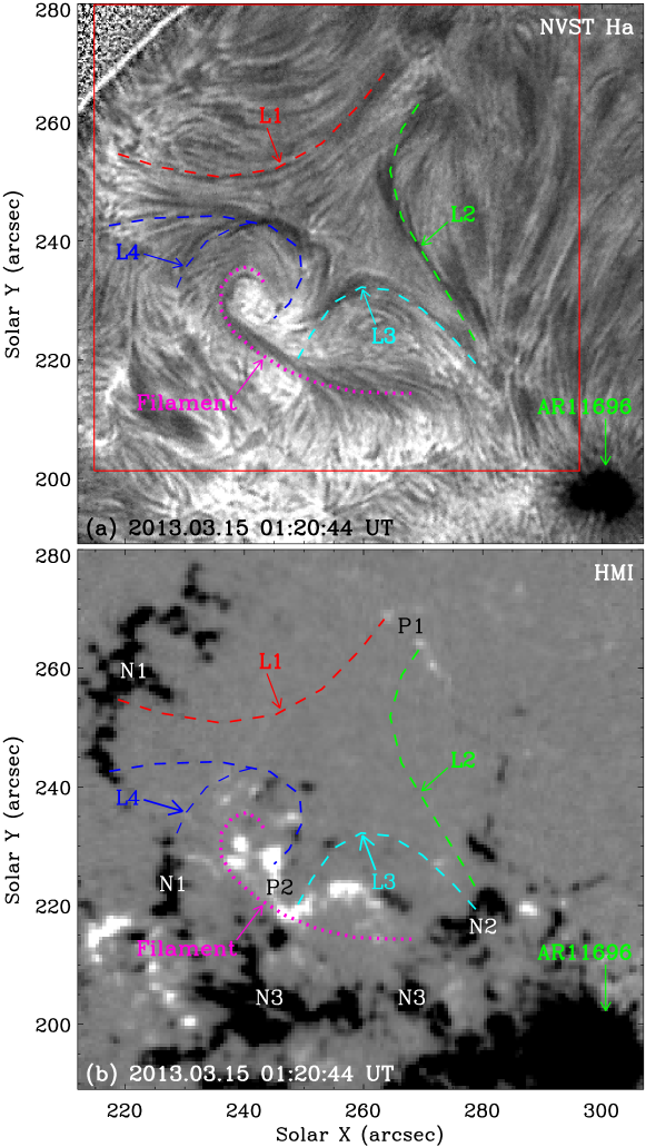
We analyze the observations that provide signatures of how a filament eruption causes magnetic reconnection to speed-up at a different location. On 2013 March 15, a saddle-like structure, located to the northeast of AR 11696, was observed by the NVST, see Figure 1(a). It is created by a set of four fibrils seen in the H images, marked separately by L1, L2, L3, and L4, see the red, green, cyan, and blue dashed lines in Figure 1(a). A curved filament is located to the southeast of the saddle-like structure, outlined by the pink dotted line in Figure 1(a). We overlay the H fibrils L1-L4 and their nearby filament on an HMI LOS magnetogram in Figure 1(b). For better descriptions, we label the positive and negative magnetic fields as P1 and P2, and N1, N2, and N3, based on the fibril connectivity, see Figure 1(b). The fibrils L1, L2, L3, and L4 connect the positive and negative magnetic fields P1 and N1, P1 and N2, P2 and N2, and P2 and N1, respectively, see the red, green, cyan, and blue dashed lines in Figure 1(b). The central positive magnetic fields P2 and their surrounding negative magnetic fields N1, N2, and N3 constitute a fan-spine magnetic field configuration, see Figures 1(b) and 9. The filament is located upon the polarity inversion line between the central positive magnetic fields P2 and the surrounding negative magnetic fields N1 and N3, see the pink dotted line in Figure 1(b).
3.1 Magnetic reconnection before the filament eruption
The H fibrils L2 and L4 constitute a saddle-type structure, see Figure 2(a). They move toward each other, and reconnect. Two sets of newly reconnected fibrils L1 and L3 then form, and retract away from the reconnection region, see the online animated version of Figure 2. No current sheet is observed in the H diagnostics in the reconnection region between fibrils L2 and L4. Along the red line AB in Figure 2(c), a time slice of H images is made, and displayed in Figure 3(a). Inward motions of fibrils L2 and L4, with mean speeds of 16-18 km s-1, see the green dotted lines in Figure 3(a), toward the reconnection region, denoted by the red dashed line in Figure 3(a), are clearly identified. Along the green line CD in Figure 2(d), another time slice of H images is obtained, and shown in Figure 3(b). At the same time, outward motions of the newly reconnected fibrils L1 and L3, with mean speeds of 24-26 km s-1, see the green dotted lines in Figure 3(b), away from the reconnection region, denoted by the red dashed line in Figure 3(b), are evidently detected. Moreover, topological reconfiguration of the fibrils by reconnection, e.g., from fibrils L4 to L3 and L1, is observed, see Figures 2(a)-(b) and (e)-(f) and the online animated version of Figure 2. Along the pink and cyan lines EF and GH in Figures 2(b) and (e), time slices of H images are made, and illustrated in Figures 3(c) and (d), respectively. The fibrils L4 reconnect with L2, and then separately turn into L3 and L1, with mean moving speeds of 7 km s-1 and 13 km s-1, see the blue dotted lines in Figures 3(c)-(d).
The process of magnetic reconnection is also observed by AIA, see Figure 4. Four sets of coronal loops L1-L4 are recorded in AIA EUV images, forming a saddle-like structure, consistent with the H fibrils L1-L4, see Figure 4(a). In the same manner, the loops L2 and L4 constitute an X-type structure, see the red dotted lines in Figure 4(c). At the interface of these two loops, magnetic reconnection takes place, see the online animated version of Figure 7. Along the cyan line IJ in Figure 4(a), a time slice of AIA 304 Å images is made, and displayed in Figure 5(a). Different from the H observations, motions of the EUV loops toward the reconnection region are hard to observe, see the online animated version of Figure 7. Nevertheless, the inward motion of loops L2, similar to the H fibrils L2, with a mean speed of 33 km s-1, see the blue dotted line in Figure 5(a), toward the reconnection region, marked by the purple dashed line in Figure 5(a), is still identified.
In the reconnection region, a current sheet forms, denoted by green solid arrows in Figure 4. In the particular snapshot, i.e., at 01:33:11 UT, it has a width of 2 Mm, and a length of 7.2 Mm in AIA 171 Å images, see Figure 4(c). Here, the length of current sheet is measured between two cusp-shaped structures at the ends of current sheet, marked by red pluses in Figure 4(c). For the width of current sheet, first we get the intensity profile in the AIA 171 Å channel perpendicular to the current sheet, e.g., along the purple line in Figure 4(c). Employing the intensity surrounding the current sheet, we calculate the background emission, and subtract it from the intensity profile. We fit the residual intensity profile using a single Gaussian, and obtain the full width at half maximum (FWHM) of the single Gaussian fit as the current sheet width. The magnetic reconnection rate, the ratio of the width and the length of the current sheet (Parker, 1957), is thus 0.28. The current sheet appears in most AIA EUV channels, except the higher-temperature channels, e.g., 335 and 94 Å, see Figure 4 and the online animated version of Figure 7. In the blue rectangle enclosing the current sheet in Figure 4(e), the light curves of the AIA 304, 131, 171, 193, and 211 Å channels are calculated, and shown in Figure 5(c). Considering the influence of background emission, similar temporal evolution of the AIA EUV light curves are identified. They reach the peaks at almost the same time, see the blue vertical dashed line in Figure 5(c). The current sheet repeatedly appears and disappears, see the online animated version of Figure 7, with a mean period of 8 minutes, obtained from the wavelet analysis of the AIA 304 Å light curve in Figure 5(c). Same as before, the well-developed current sheets are measured using AIA 171 Å images. They have the width of 1-2 Mm with a mean value of 1.5 Mm, the length of 5.3-7.2 Mm with a mean value of 6.4 Mm, and the reconnection rate of 0.18-0.3 with a mean value of 0.24.
As the current sheet is not observed in the AIA higher-temperature channels, e.g., 94 and 335 Å, plasma at that location could be cooler than 2.5 MK, the characteristic temperature of AIA 335 Å channel. The current sheet in AIA 131 Å images, see Figure 4(b), hence shows plasma with the lower characteristic temperature (0.6 MK) of AIA 131 Å channel. Using six AIA EUV channels, including 94, 335, 211, 193, 171, and 131 Å, we analyze the temperature and emission measure (EM) of the current sheet. Here, we employ the differential EM (DEM) analysis using “xrt_dem_iterative2.pro” (Cheng et al., 2012). The current sheet region, enclosed by the red rectangle in Figure 4(b), is chosen to compute the DEM. The region out of the current sheet, enclosed by the purple rectangle in Figure 4(b), is chosen for the background emission that is subtracted from the current sheet region. In each region, the DN counts in each of the six AIA channels are temporally normalized by the exposure time and spatially averaged over all pixels. The DEM curve of the current sheet region is displayed in Figure 5(e). Consistent with the AIA imaging observations, the DEM shows a lack of hot plasma component in the current sheet, see the black curve in Figure 5(e). The average DEM-weighed temperature and EM are 2 MK and 2.51027 cm-5, respectively.
Using the EM, the number density () of current sheet is estimated using , where is the LOS depth of current sheet. Assuming that the depth equals the width () of current sheet, then the density is . Employing EM=2.51027 cm-5 and W=2 Mm, we obtain the density to be 3.5109 cm-3. The thermal energy (TE) of current sheet is also calculated using TE=npkBVT. Here kB is Boltzmann’s constant, V volume, and T temperature increase from the temperature (T1) of reconnection inflowing structure to that (T2) of current sheet. Assuming that the current sheet is a cylinder, its volume is then V=()2L, where L is the length of current sheet. Therefore the thermal energy is TE=npkB()2L(T2-T1). As the reconnection inflow is observed mainly in H images and the current sheet is identified in EUV images, we obtain T1=104 K, the temperature of H fibrils (Leenaarts et al., 2012), and T2 to be the average DEM-weighed temperature of current sheet. Employing np=3.5109 cm-3, W=1-2 Mm, L=5.3-7.2 Mm, T2=2 MK, and T1=104 K, we calculate the thermal energy of current sheet, and get TE=(1.91.3)1025 erg.
Plasmoids appear in the current sheet, and propagate along it bi-directionally, and then further along the reconnection loops L2 and L4, see Figure 4(d) and the online animated version of Figure 7. Same as the current sheet, they are not observed in the AIA higher-temperature channels, e.g., 335 and 94 Å. Along the current sheet, see the green line KL in Figure 4(c), a time slice of AIA 171 Å images is made, and shown in Figure 5(b). It indicates that the plasmoids always form in the middle of the current sheet, marked by the red dashed line in Figure 5(b), and then move bi-directionally with mean speeds of 36-48 km s-1, see the green dotted lines in Figure 5(b). Along the blue line MN in Figure 4(c), another time slice of AIA 171 Å images is made, and illustrated in Figure 5(d). Several motions of plasmoids along the north leg of loops L2 are evidently identified, with a mean speed of 71 km s-1, see the green dotted line in Figure 5(d).
From 02:30 UT, a set of higher-lying loops L6, connecting the surrounding negative magnetic fields N1-N3 and the remote positive magnetic fields, appears in most AIA EUV channels, except 304 Å, see Figure 6(a). They are likely to be heated by nanoflares (Li et al., 2015), as no significant activity is detected associated with the brightening of loops. The current sheet, i.e., the reconnection region, is then covered by the loops L6 in these EUV channels. It, however, still appears in AIA 304 Å images, see the online animated version of Figure 7. This indicates that the reconnection between loops L2 and L4 continues to take place as before, consistent with the H observations. A set of lower-lying loops L5 overlying the filament is also detected. It connects the positive and negative magnetic fields P2 and N3, see Figures 6(a) and 9. In the AIA higher-temperature channels, e.g., 94 and 335 Å, the loops L5 and L6 gradually disappear, indicating the cooling process of heated loops (Li et al., 2015). Consistent with the previous observations, the current sheet forms in the lower-temperature, e.g., 304 Å, rather than the higher-temperature channels, e.g., 94 and 335 Å, see the online animated version of Figure 7.
3.2 Filament eruption
From 05:52 UT, the north, rather than the south, part of the filament, located to the southeast of the reconnection region, brightens, see Figure 6(b), and then erupts, see Figure 6(d). A partial eruption of the filament is thus observed (Li et al., 2016a). Along the erupting direction, see the green line PQ in Figure 6(b), a time slice of AIA 304 Å images is made, and displayed in Figure 6(g). The filament erupts with a mean projection speed of 55 km s-1, see the blue dotted line in Figure 6(g). Assuming that the filament erupts outward along the radial direction, we obtain the corrected erupting speed to be 163 km s-1, using the heliographic position N13 W15 of the erupting filament. The erupting filament is prevented eventually by the higher-lying loops L5 and L6, showing a failed filament eruption, and makes the higher-lying loops bright, see Figure 6(e) and the online animated version of Figure 7. Moreover, the failed filament eruption may also be caused by the reconnection between the erupting filament and its overlying loops (Li et al., 2016a; Yan et al., 2020b). Two flare ribbons and post-flare loops, associated with the filament eruption, appear, see Figures 6(c) and (e). The south flare ribbon moves away from the polarity inversion line of the positive and negative magnetic fields P2 and N3, with a mean speed of 42 km s-1, see the green dotted line in Figure 6(g).
The filament eruption pushes away the higher-lying loops L6 covering the reconnection region, see Figure 6(f) and the online animated version of Figure 7. It thus leads to a disturbance propagating outward across the reconnection region. Along the propagating direction VW in the blue rectangle in Figure 6(f), a time slice of AIA 211 Å images is measured, and shown in Figure 6(h). It indicates that the loops L6 is pushed away with a mean moving speed of 290 km s-1 by the propagating disturbance caused by the filament eruption, see the blue dotted line in Figure 6(h). A dimming region then forms, and the reconnection region, e.g., the current sheet, reappears in these AIA EUV channels, e.g., 171, 193, and 211 Å, see the online animated version of Figure 7.
3.3 Magnetic reconnection after the filament eruption
After the filament eruption, the current sheet between loops L2 and L4 has the width and length of 2 Mm and 3.5 Mm at 06:18:35 UT, and thus a reconnection rate of 0.57, see Figure 7(c). Here, the width is similar to the current sheet widths (1-2 Mm), the length is, however, smaller than the current sheet lengths (5.3-7.2 Mm), and the reconnection rate is much larger than the reconnection rates (0.18-0.3), before the filament eruption. The current sheet, different from those occurring in the AIA low-temperature EUV channels before the filament eruption, appears in all AIA EUV channels, marked by the green solid arrows in Figure 7. Same as in Section 3.1, in the blue rectangle enclosing the reconnection region in Figure 7(e), the light curves of the AIA 94, 335, 211, 193, 171, 131, and 304 Å channels are calculated, and displayed in Figure 8(a). Here, the AIA 211, 193, and 171 Å light curves before the filament eruption, denoted by the red vertical dotted line in Figure 8(a), are not measured, because before the filament eruption the reconnection region is covered by the higher-lying loops L6 in these channels, see Section 3.1. Before the filament eruption, the AIA 94 Å and 335 Å light curves keep constant, indicating that no current sheet appears in these AIA higher-temperature channels. The AIA 304 Å and 131 Å light curves, however, evolve due to the appearance of current sheet in these lower-temperature channels. Right after the filament eruption, the AIA 335, 211, 193, and 171 Å light curves decrease evidently, showing a dimming, as the higher-lying loops L6, covering the reconnection region, are pushed away by the propagating disturbance caused by the filament eruption, see also Figures 6(f) and (h). All the light curves then exhibit rapid rise and reach the peaks. Among them, the AIA 94 Å light curve reaches the peak at 06:09:37 UT, see the green vertical dashed line in Figure 8(a), 2.3 minutes later than the AIA 304 Å light curve that peaks at 06:07:19 UT, see the blue vertical dashed line in Figure 8(a). Affected by the brightening of higher-lying loops caused by the filament eruption, see Section 3.2, the AIA 335 Å light curve reaches the peak several minutes later than the other light curves. It, however, has a small peak at 06:07:26 UT, identical to the peak of the AIA 304 Å light curve, see Figure 8(a). In addition, a much bright reconnection region is detected simultaneously in H observations, see the online animated version of Figure 2.
As the current sheet appears in all AIA EUV channels, it, therefore, may contain plasma with both of the high and low temperature. The current sheet region, enclosed by the red rectangle in Figure 7(d), is chosen to compute the DEM. The region out of the current sheet, enclosed by the purple rectangle in Figure 7(d), is selected for the background emission that is subtracted from the current sheet region. The DEM curve of the current sheet region is shown in Figure 8(c). It indicates that more plasma with higher temperature and less plasma with lower temperature is detected in the current sheet, comparing to that in Figure 5(e). The average DEM-weighed temperature and EM are 5.5 MK and 1.71028 cm-5, respectively. Both these quantities are significantly higher than those of current sheet before the filament eruption (2 MK and 2.51027 cm-5). Similar to Section 3.1, the density of current sheet is also estimated to be 9.2109 cm-3 by using the EM, under the assumption that the LOS depth (D) of the current sheet equals its width (W=2 Mm). It is larger than that of current sheet before the filament eruption (3.5109 cm-3). Using np=9.2109 cm-3, W=2 Mm, L=3.5 Mm, T2=5.5 MK, and T1=104 K, we also calculate the thermal energy of current sheet, and obtain the value to be TE=1.11026 erg. It is also larger than that of current sheet before the filament eruption (1.91.31025 erg).
In the current sheet, plasmoids appear and move along it and the reconnection loops, see Figure 6(d) and the online animated version of Figure 7. The north endpoint of loops L2, enclosed by the pink circles, then brightens, see Figure 7(h). Along the green line RS in Figure 7(c), a time slice of AIA 171 Å images is made, and displayed in Figure 8(b). It shows that more plasmoids moving along the north leg of loops L2 are detected, comparing with that in Figure 5(d), with a similar mean speed of 70 km s-1, see the green dotted line in Figure 8(b). Moreover, the plasmoids, different from those appearing in the AIA lower-temperature EUV channels before the filament eruption, see Section 3.1, appear in all AIA EUV channels. More hotter plasmoids are thus generated in the current sheet after the filament eruption. Comparing all the results before and after the filament eruption, see Sections 3.1 and 3.3, we conclude that the reconnection between loops L2 and L4 is significantly accelerated by the filament eruption occurring to the southeast of the reconnection region.
4 Summary and discussion
Employing the H images from NVST, and the AIA images and HMI LOS magnetograms from SDO, we study the reconnection between fibrils (loops) L2 and L4, and its nearby filament eruption. The reconnection accelerated by the filament eruption is then reported. In H images, a saddle-like structure, consisting of four sets of fibrils L1-L4, is observed. The fibrils L2 and L4 from opposite sides of the saddle region move together, and reconnect. The newly reconnected fibrils L1 and L3 then form, and retract away from the reconnection region. In AIA EUV images, similar loops L1-L4 and their evolution are identified. At the interface of loops L2 and L4, the current sheet repeatedly forms and disappears. Magnetic reconnection takes place in the current sheet. Plasmoids appear in the current sheet, and propagate along it, and then further along the reconnection loops. A filament, located to the southeast of the reconnection region, partially erupts, and leads to a flare. It is then prevented by the overlying loops as a failed filament eruption. After the filament eruption, a hotter, shorter current sheet forms with a much larger reconnection rate, where more hotter plasmoids appear. Based on the NVST H images, and the SDO AIA EUV images and HMI LOS magnetograms, a schematic diagram of the magnetic reconnection between fibrils (loops) and its nearby filament eruption is demonstrated in Figure 9. Here, the red star represents the reconnection point between magnetic field lines of loops L2 and L4.
A small-scale reconnection event among a saddle-like structure is observed by NVST. Similar to the small-scale reconnection events previously reported (Yang et al., 2015a; Yang & Xiang, 2016), inward and outward motions of H fibrils toward and away from the reconnection region are evidently detected, see Section 3.1. The reconnection inflowing and outflowing speeds of 17 km s-1 and 25 km s-1 are consistent with those of the fast reconnection event in Yang et al. (2015a). Different from Yang et al. (2015a), in this study the current sheet appears only in the AIA EUV channels, rather than the H channel, see Section 3.1. This indicates that the current sheet is significantly heated during the reconnection process (Li et al., 2016a, b; Xue et al., 2020). The width (1-2 Mm) and length (3.5-7.2 Mm) of current sheets are identical to those in Xue et al. (2016, 2020), but larger than those in Yang et al. (2015a) and Xue et al. (2018). Moreover, the reconnection rate (0.18-0.57) is similar to those in Xue et al. (2016, 2018), but larger than those in Xue et al. (2020). Many plasmoids form in the current sheet, suggesting the presence of plasmoid instabilities during the process of magnetic reconnection (Kumar & Cho, 2013; Li et al., 2016a; Peter et al., 2019). They propagate along the current sheet bi-directionally, and then further along the reconnection loops with a mean speed of 70 km s-1. The moving speed here is consistent with those in Yang et al. (2015a) and Xue et al. (2020), but smaller than those in Li et al. (2016a).
Magnetic reconnection accelerated by nearby filament eruption is observed. After the filament eruption, the length of current sheet decreases significantly from 5.3-7.2 Mm to 3.5 Mm. The reconnection rate, however, increases largely from 0.18-0.3 to 0.57, see Sections 3.1 and 3.3. The enhancements of the AIA EUV light curves in the reconnection region after the filament eruption, see Figures 4(c) and 7(a), suggest the increase of temperature and/or density of plasma in the current sheet. The current sheet appears in the AIA higher-temperature channels, e.g., 335 and 94 Å, after rather than before the filament eruption. It is thus heated to much higher temperature after the filament eruption. This is also supported by the DEM curves of current sheet before and after the filament eruption, e.g., the average DEM-weighed temperature of current sheet increases from 2 MK to 5.5 MK. The increase of current sheet density from 3.5109 cm-3 to 9.2109 cm-3 after the filament eruption shows that more plasma (np()2L) from (4.73.2)1034 to 11035 is heated to higher temperature. More thermal energy of current sheet converted by reconnection after (1.11026 erg) than before ((1.91.3)1025 erg) the filament eruption is then achieved. In addition, more hotter plasmoids form in the current sheet after the filament eruption during the same time intervals, see Figures 5(d) and 8(b). This indicates that more plasma is accelerated during the reconnection process. More kinetic energy is hence converted by reconnection after the filament eruption.
Magnetic reconnection may be accelerated by the fast MHD wave caused by filament eruption. Nakariakov et al. (2006) suggested that the fast wave coming into the magnetic null point from the outside leads to the increase of electric current density. The increasing electric current then efficiently induces plasma micro-instabilities of various kinds, and hence produces anomalous resistivity, which efficiently triggers the reconnection. Fast mode MHD waves generated by filament eruptions are indeed widely reported (e.g., Liu et al., 2010b; Li et al., 2012; Shen et al., 2018). In this study, the higher-lying loops covering the reconnection region in the AIA EUV channels are pushed away right after the filament eruption, see Section 3.2. This suggests that the filament eruption leads to a disturbance propagating outward across the reconnection region, that could be related to fast mode MHD wave. Using vA=, we calculate the Alfvn speed near the reconnection region, where B is the magnetic field strength, and mp is the proton mass. Employing the magnetic field strength B=(32) G in the corona (Yang et al., 2020), and the coronal density np=(10.5)109 cm-3, less than the current sheet density (3.5109 cm-3) before the filament eruption, the Alfvn speed is obtained to be vA=(272216) km s-1. It is consistent with the propagating speed (290 km s-1) of the disturbance. This propagating disturbance is hence likely to represent the fast-mode MHD wave driven by the filament eruption. The fast wave comes into the current sheet, increases its electric current density (Nakariakov et al., 2006), and accelerates the magnetic reconnection. It could also enhance turbulent plasma motions at the current sheet, leading to a turbulent reconnection (Chitta & Lazarian, 2020). Additionally, the propagating disturbance may also push more magnetic flux of loops (fibrils) L4, and thus more magnetic energy, into the reconnection region (Zhou et al., 2017). All these effects will play a role in liberating magnetic energy with a larger reconnection rate. The released magnetic energy will then be converted to other forms of energy, e.g., thermal and kinetic.


References
- Chen et al. (2016) Chen, H. D., Zhang, J., Li, L. P., et al. 2016, ApJ, 818, L27
- Chen (2011) Chen, P. F. 2011, Living Reviews in Solar Physics, 8, 1
- Chen & Priest (2006) Chen, P. F. & Priest, E. R. 2006, Sol. Phys., 238, 313
- Cheng et al. (2018) Cheng, X., Li, Y., Wan, L. F., et al. 2018, ApJ, 866, 64
- Cheng et al. (2012) Cheng, X., Zhang, J., Saar, S. H., et al. 2012, ApJ, 761, 62
- Chitta & Lazarian (2020) Chitta, L. P. & Lazarian, A. 2020, ApJ, 890, L2. doi:10.3847/2041-8213/ab6f0a
- Ciaravella & Raymond (2008) Ciaravella, A. & Raymond, J. C. 2008, ApJ, 686, 1372
- Feng et al. (2012) Feng, S., Ji, K. F., Deng, H., et al. 2012, Journal of Korean Astronomical Society, 45, 167
- Hong et al. (2019) Hong, J. C., Yang, J. Y., Chen, H., et al. 2019, ApJ, 874, 146
- Huang et al. (2018) Huang, Z. H., Mou, C. Z., Fu, H., et al. 2018, ApJ, 853, L26
- Innes et al. (2003) Innes, D., McKenzie, D., & Wang, T. 2003, Sol. Phys., 217, 267
- Kong et al. (2018) Kong, D. F., Pan, G. M., Yan, X. L., et al. 2018, ApJ, 863, L22
- Kumar & Cho (2013) Kumar, P. & Cho, K.-S. 2013, A&A, 557, A115
- Leenaarts et al. (2012) Leenaarts, J., Carlsson, M., & Rouppe van der Voort, L. 2012, ApJ, 749, 136
- Lemen et al. (2012) Lemen, J. R., Title, A., Akin, D., et al. 2012, Sol. Phys., 275, 17
- Li et al. (2016c) Li, D., Ning, Z. J., & Su, Y. 2016c, Ap&SS, 361, 301
- Li et al. (2014) Li, L. P., Peter, H., Chen, F., et al. 2014, A&A, 570, A93
- Li et al. (2015) Li, L. P., Peter, H., Chen, F., et al. 2015, A&A, 583, A109. doi:10.1051/0004-6361/201526912
- Li et al. (2019) Li, L. P., Peter, H., Chitta, L. P., et al. 2019, ApJ, 884, 34
- Li & Zhang (2009) Li, L. P. & Zhang, J. 2009, ApJ, 703, 877
- Li et al. (2012) Li, L. P., Zhang, J., Li, T., et al. 2012, A&A, 539, A7
- Li et al. (2016a) Li, L. P., Zhang, J., Peter, H., et al. 2016a, Nature Physics, 12, 847
- Li et al. (2018a) Li, L. P., Zhang, J., Peter, H., et al. 2018a, ApJ, 864, L4
- Li et al. (2018b) Li, L. P., Zhang, J., Peter, H., et al. 2018b, ApJ, 868, L33
- Li et al. (2016b) Li, L. P., Zhang, J., Su, J. T., et al. 2016b, ApJ, 829, L33
- Lin & Forbes (2000) Lin, J. & Forbes, T. G. 2000, J. Geophys. Res., 105, 2375
- Lin et al. (2005) Lin, J., Ko, Y.-K., Sui, L., et al. 2005, ApJ, 622, 1251
- Liu et al. (2010a) Liu, R., Lee, J., Wang, T., et al. 2010a, ApJ, 723, L28
- Liu et al. (2010b) Liu, W., Nitta, N. V., Schrijver, C. J., et al. 2010b, ApJ, 723, L53
- Liu et al. (2014) Liu, Z., Xu, J., Gu, B.-Z., et al. 2014, Research in Astronomy and Astrophysics, 14, 705-718
- Masuda et al. (1994) Masuda, S., Kosugi, T., Hara, H., et al. 1994, Nature, 371, 495
- McKenzie (2000) McKenzie, D. E. 2000, Sol. Phys., 195, 381
- McLaughlin et al. (2009) McLaughlin, J. A., De Moortel, I., Hood, A. W., et al. 2009, A&A, 493, 227
- McLaughlin et al. (2018) McLaughlin, J. A., Nakariakov, V. M., Dominique, M., et al. 2018, Space Sci. Rev., 214, 45
- Müller et al. (2017) Müller, D. A. N., Nicula, B., Felix, S., et al. 2017, A&A, 606, A10
- Nakariakov et al. (2006) Nakariakov, V. M., Foullon, C., Verwichte, E., et al. 2006, A&A, 452, 343
- Ni et al. (2020) Ni, L., Ji, H., Murphy, N., & Jara-Almonte, J. 2020, Proc. R. Soc. A., 476, 20190867
- Parker (1957) Parker, E. N. 1957, J. Geophys. Res., 62, 509
- Pesnell et al. (2012) Pesnell, W. D., Thompson, B. J., & Chamberlin, P. C. 2012, Sol. Phys., 275, 3
- Peter et al. (2019) Peter, H., Huang, Y.-M., Chitta, L. P., et al. 2019, A&A, 628, A8
- Priest (2014) Priest, E. 2014, Magnetohydrodynamics of the Sun, by Eric Priest, Cambridge, UK: Cambridge University Press, 2014
- Priest & Forbes (2000) Priest, E. & Forbes, T. 2000, Magnetic reconnection : MHD theory and applications / Eric Priest
- Schou et al. (2012) Schou, J., Scherrer, P. H., Bush, R. I., et al. 2012, Sol. Phys., 275, 229
- Shen et al. (2018) Shen, Y. D., Liu, Y., Song, T., et al. 2018, ApJ, 853, 1
- Shen et al. (2019) Shen, Y. D., Qu, Z., Yuan, D., et al. 2019, ApJ, 883, 104
- Shibata (1999) Shibata, K. 1999, Ap&SS, 264, 129
- Song et al. (2012a) Song, H. Q., Chen, Y., Li, G., et al. 2012a, Physical Review X, 2, 021015
- Song et al. (2012b) Song, H. Q., Kong, X. L., Chen, Y., et al. 2012b, Sol. Phys., 276, 261
- Su et al. (2013) Su, Y., Veronig, A. M., Holman, G. D., et al. 2013, Nature Physics, 9, 489
- Takasao et al. (2012) Takasao, S., Asai, A., Isobe, H., et al. 2012, ApJ, 745, L6
- Tian et al. (2014) Tian, H., Li, G., Reeves, K. K., et al. 2014, ApJ, 797, L14
- Tsuneta et al. (1992) Tsuneta, S., Hara, H., Shimizu, T., et al. 1992, PASJ, 44, L63
- Xiang et al. (2016) Xiang, Y. Y., Liu, Z., & Jin, Z. Y. 2016, New A, 49, 8
- Xue et al. (2016) Xue, Z. K., Yan, X. L., Cheng, X., et al. 2016, Nature Communications, 7, 11837
- Xue et al. (2019) Xue, Z. K., Yan, X. L., Jin, C. L., et al. 2019, ApJ, 874, L27
- Xue et al. (2018) Xue, Z. K., Yan, X. L., Yang, L. H., et al. 2018, ApJ, 858, L4
- Xue et al. (2020) Xue, Z. K., Yan, X. L., Yang, L. H., et al. 2020, A&A, 633, A121
- Yamada et al. (2010) Yamada, M., Kulsrud, R., & Ji, H. 2010, Reviews of Modern Physics, 82, 603
- Yan et al. (2020a) Yan, X. L., Liu, Z., Zhang, J., et al. 2020a, Sci. China Technol. Sci., 63, https://doi.org/10.1007/s11431-019-1463-6
- Yan et al. (2020b) Yan, X. L., Xue, Z. K., Cheng, X., et al. 2020b, ApJ, 889, 106. doi:10.3847/1538-4357/ab61f3
- Yan et al. (2018) Yan, X. L., Yang, L., Xue, Z., et al. 2018, ApJ, 853, L18
- Yang et al. (2019) Yang, B., Yang, J. Y., Bi, Y., et al. 2019, ApJ, 887, 220
- Yang et al. (2017) Yang, L. H., Yan, X. L., Li, T., et al. 2017, ApJ, 838, 131
- Yang & Xiang (2016) Yang, S. H. & Xiang, Y. Y. 2016, ApJ, 819, L24
- Yang et al. (2015a) Yang, S. H., Zhang, J., & Xiang, Y. 2015a, ApJ, 798, L11
- Yang et al. (2015b) Yang, Y. F., Qu, H. X., Ji, K. F., et al. 2015b, Research in Astronomy and Astrophysics, 15, 569
- Yang et al. (2020) Yang, Z., Bethge, C., Tian, H., et al. 2020, Science, 369, 694
- Yokoyama et al. (2001) Yokoyama, T., Akita, K., Morimoto, T., et al. 2001, ApJ, 546, L69
- Zhang et al. (2013) Zhang, J., Yang, S. H., Li, T., et al. 2013, ApJ, 776, 57
- Zheng et al. (2018) Zheng, R. S., Chen, Y., Huang, Z. H., et al. 2018, ApJ, 861, 108
- Zhong et al. (2019) Zhong, S. H., Hou, Y. J., & Zhang, J. 2019, ApJ, 876, 51
- Zhou et al. (2017) Zhou, G. P., Zhang, J., Wang, J. X., et al. 2017, ApJ, 851, L1