Magnetic Bloch oscillations in a non-Hermitian quantum Ising chain
Abstract
We investigate the impacts of an imaginary transverse field on the dynamics of magnetic domain walls in a quantum Ising chain. We show that an imaginary field plays a similar role as a real transverse field in forming a low-lying Wannier-Stark ladder. However, analytical and numerical calculations of the time evolutions in both systems show that the corresponding Bloch oscillations exhibit totally different patterns for the same initial states. These findings reveal the nontrivial effect of non-Hermiticity on quantum spin dynamics.
I Introduction
Bloch oscillation (BO) describes the periodic motion of a wave packet subjected to an external force in a lattice. This phenomenon was first noted by Bloch and Zener when they studied the electrical properties of crystals [1, 2]. When an external electric field is applied to a perfect crystal lattice, the localized eigenstates with a ladder-like energy spectrum emerge, known as the Wannier-Stark (WS) ladder [3]. These states are closely related to the BOs, which can be understood as the periodic motion of a wave packet within the WS ladder, as an external field causes the wave packet to transition between different WS states and exhibit oscillatory behavior in terms of position and velocity. Experimentally, BOs were observed in a semiconductor superlattice [4], ultracold atoms in the optical lattice [5, 6, 7, 8] and many other systems sequentially [9, 10, 11, 12, 13]. It turns out that BO is a universal wave phenomenon. In the magnetic systems, BOs appear in the form of the magnetic domain-wall oscillations. As a nonequilibrium dynamic phenomenon in quantum many-body systems, magnetic BOs in the quantum spin chains have attracted much attention from researchers [14, 15, 16, 17, 18, 19, 20, 21, 13]. Notably, inelastic neutron scattering experiments have provided evidence for the existence of magnetic BOs in the magnetically identical material [13].
In recent years, non-Hermitian physics have attracted much attention from various research areas [22, 23, 24, 25, 26, 27, 28, 29, 30, 31, 32, 33], and BOs have been investigated in a range of non-Hermitian systems, including photonic lattices with gain or loss [22, 34, 35], tight-binding chains with an imaginary gauge field [36, 37, 38], and non-Hermitian frequency lattices induced by complex photonic gauge fields [26]. Classical systems such as photonics, mechanics and electrical circuits can be used to simulate non-Hermitian wave physics at the single-particle level, while in the quantum systems non-Hermitian Hamiltonians are mainly explained as the effective descriptions of open quantum systems [27], and have been experimentally realized in the systems of superconducting quantum circuits [39, 40], nitrogen-vacancy centers in diamonds [41, 29] and ultracold atoms [42, 43]. Moreover, it was proposed that an imaginary field in a spin chain can be implemented by a scheme similar to heralded entanglement protocols [24]. More recently, researchers have shown that complex fields in quantum spin models have unique impacts on the physical properties of the systems [44, 45, 46, 47, 48, 49, 50, 51, 52, 53], for example, by driving a quantum phase transition and altering the phase diagram of the system. However, to the best of our knowledge, the BO in a non-Hermitian quantum spin chain has not yet been explored.
In this paper, we investigate the BOs of magnetic domain walls in a non-Hermitian quantum Ising chain. The model considered is a quantum Ising chain with real longitudinal and imaginary transverse fields. We show that in the small-field region, i. e., when the strengths of two fields are much smaller than the Ising coupling, as well as in the -symmetric parameters region that guarantees a full real spectrum, the low-energy dynamics of the magnetic domain walls are captured by a single-particle effective Hamiltonian, through which the physical mechanism of magnetic BOs is revealed. For real and imaginary transverse fields, the eigenstates of the effective Hamiltonian are both localized states with ladder-like energy spectra, forming the WS ladders. Analytical analysis and numerical calculation of the time evolutions show the occurrence of magnetic breathing and BO modes in the non-Hermitian quantum Ising chain by appropriately selecting the initial states. It is shown that for the non-Hermitian quantum Ising chain, the dynamics for the Kronecker delta initial state is a breathing mode, while the Gaussian state remains stationary, which is totally different from the oscillation of the domain wall in a Hermitian quantum Ising chain. Interestingly, for the Bessel initial state, the BO mode appears, and the amplitude can be modulated by the strength of the imaginary transverse field and the localization length of the initial state.
This paper is organized as follows. In Sec. II, we start by introducing the Hamiltonian of the quantum Ising chain with an imaginary transverse field, and derive the effective Hamiltonian and its solution. In Sec. III, we analyze the dynamics of BOs for three types of initial states on the basis of the effective Hamiltonian, while Sec. IV presents the numerical results of the dynamics for the quantum spin chain. Finally, we conclude our findings in Sec. V.
II Model and effective Hamiltonian
The model we consider is a quantum spin chain of length with the Hamiltonian
| (1) |
where
| (2) |
represents a spin chain in longitudinal magnetic field , and with ferromagnetic Ising coupling . For simplicity, we set in the following discussion. Here () are the Pauli operators on site , while
| (3) |
is a transverse magnetic field term. In this paper, we consider both the Hermitian and non-Hermitian systems, when the transverse fields are taken as real and imaginary, respectively. We would like to point out that the Hamiltonian is different from that of the Yang-Lee Ising spin model, which exhibits Lee-Yang zeros [54, 55, 56, 57, 58, 59, 60]; in this model, the longitudinal field is imaginary, and the transverse field is real instead. When , the Hamiltonian reduces to the transverse field Ising chain, which is exactly solvable through the Jordan-Wigner transformation when the periodic boundary condition is applied, and serves as a unique paradigm for understanding the quantum phase transition [61]. A nonzero longitudinal field term involves nonlocal operators in the fermion representation, and thus breaks the solvability of the model.
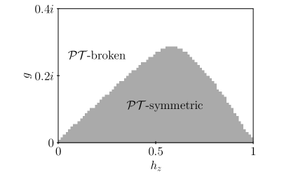
Imaginary fields in quantum spin systems have been discussed in many experimental and theoretical works [24, 41, 29, 42, 43, 62, 63, 64]. In the framework of open quantum system dynamics, the imaginary transverse field arises in the no-click limit of the stochastic quantum jump trajectories when is measured [62, 63, 64], and can be interpreted as either dissipation or measurement rate. In this case, the resulted non-Hermitian Hamiltonian respects symmetry, that is, , with being the parity operator, and being the complex conjugation operator. This guarantees a full real spectrum in a certain region of system parameters [65, 66, 67, 57], which is the so-called -symmetric region where the eigenstates remain unchanged under the action of the operator. Beyond this region, the eigenvalues occur in complex conjugate pairs and the corresponding eigenstates change under the action of the operator. Due to the lack of solvability in the model, the phase boundary of these two regions cannot be obtained analytically. Nevertheless, it is expected that the system possesses a full real spectrum when is small compared to other system parameters. In Fig. 1, we presented the numerical result of the phase diagram of broken and unbroken symmetry for a finite-size system. The -symmetric region is determined by condition , where is the energy level of system .
In this paper, we are concerned with the dynamics in the low-energy subspace as well as in the -symmetric parameters region of the model. Thus, we content ourselves with a perturbation solution through seeking for an effective Hamiltonian describing the low-energy dynamics. To proceed, we concentrate on the weak-field situation with , and treat the transverse field term as a perturbation in the following discussion.
We note that all the eigenstates of can be written in the tensor product form with fixed numbers of spins that are parallel or antiparallel to the direction. The ground state of is with energy . We focus on the low-energy subspace that consists of states having one magnetic domain wall. Here represent two types of domain-wall states:
| (4) |
with the lowering operator, and the spatial position of the domain wall. The corresponding energy is . The action of on this basis yields
| (5) | |||||
Here the ellipsis dots “…” represent the terms containing the basis states with more than one domain wall, which have at least energy difference compared to the states in . Thus, we are able to adiabatically eliminate these states and project the Hamiltonian into the subspace . The effective Hamiltonian is given by [68]
| (6) |
where the projectors are defined as and . The second term in Eq. (6) that is proportional to is discarded, considering the solvability of the effective Hamiltonian and is a small quantity. Up to first order, the effective Hamiltonian has the explicit form
| (7) | |||
This indicates that the transverse field acts as a hopping coefficient for the magnetic domain wall, while the strength of the longitudinal field plays the role of a skew potential. Next, we investigate the dynamics in subspace, and denote for simplicity. The analysis is similar for that of subspace. In the absence of the skew potential , the -periodic spectrum is for the Bloch wave of magnetic excitation . For a real , the semiclassical picture of BOs has been well understood [1, 2]. However, for an imaginary , the semiclassical picture should be understood in the framework of a modified equation of motion for expectation values, and the acceleration theorem holds only on average in time [37, 38].
The eigenstate of the Hamiltonian can be expanded as , and the stationary Schrödinger equation gives the recursive relation for the expansion coefficients
| (8) |
with and . The boundary condition is . We identify that Eq. (8) is the recursive formula of the Bessel function. Since the boundary effect is not involved in the dynamics that we will investigate in the next section, we assume an infinite chain in the following analytical analysis for convenience. Then the solution can be written as
| (9) |
which is the Bessel function of the first kind. Notably, the argument is imaginary for a non-Hermitian system. These eigenstates can be related by the spatial translation operation, that is, with the translation operator defined as . Then the eigenstates for the Hamiltonian are
| (10) |
with energy , which is equally spaced and independent of .
Similarly, the eigenstate of the Hamiltonian with energy is
| (11) |
which establishes a biorthonormal basis set satisfying
| (12) | |||||
| (13) |
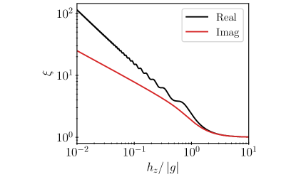
It is well known that the eigenstates are localized for a Hermitian WS ladder [69]. Thus, it can be reasonably inferred that this is also the case for an imaginary . This can be confirmed by the localization length for the eigenstate, which is defined as [70, 19]
| (14) |
For an infinite system, is independent of energy. Also, of the localized state is independent of when is large enough. In Fig. 2, we present the numerical results of the localization length of the eigenstates for the real and imaginary fields , respectively. We can see that for both cases, a nonzero longitudinal field induces the localization of the eigenstates, which is more pronounced for an imaginary . The localization of eigenstates is crucial for the upcoming discussion.
III Analyses for the oscillation dynamics
In this section, we investigate the dynamics of magnetic BOs in a non-Hermitian quantum spin chain through an analytical analysis of the effective Hamiltonian. The characteristics of eigenstate localization and equal spacing of energy levels are both crucial for the construction of the initial excitation of the magnetic BOs.
We consider the initial states
| (15) |
with three types of distributions representing the domain wall localized at site : (i) the delta function ; (ii) the broad Gaussian distribution where is a normalization coefficient, characterizes the width of the distribution, and is the wavevector; and (iii) the Bessel distribution with a complex argument . According to the Schrödinger equation, the evolved state can be formally written as
| (16) | |||||
From the solution in Eqs. (10)-(13), the propagator under the biorthonormal basis can be computed as follows:
| (17) | |||||
and then using Graf’s addition theorem [71, 72] for the Bessel functions in the summation of index , we arrive at
| (18) |
Here, a -independent overall phase factor is discarded. Obviously, the propagator is periodic with a Bloch period .
III.1 Kronecker delta initial state
Then, for the initial state , the evolved state is simply
According to the properties of Bessel functions, the width of the domain wall periodically widens and narrows within the range
| (20) |
for both real and imaginary field with period , which is the Bloch breathing mode. The profile of the evolved state here is independent of the particular value of initial position .
III.2 Gaussian initial state
The evaluation of the time evolution for the initial state with Gaussian distribution is not straightforward. Some approximations are needed. To do this, we first Fourier transform the time-evolution equation into space:
| (21) | |||||
Assume that the spatial localization of the initial distribution is weak, that is, , so that the summation of can be approximately replaced by integration. By doing this, we achieve
| (22) |
Again, since is assumed, the momentum distribution is sharply localized around . Then, we can expand the factor in the argument of the exponential around up to the first order, and the evolved state in real space can be obtained as
| (23) | |||
where
| (24) | |||||
| (25) |
For a real , the center of the wave packet in real space oscillates in the form of a cosine function with period and amplitude , which is the BO mode. However, for an imaginary , the center of the wave packet remains stationary at the initial position for any initial wavevector . Thus, in the following, we seek for a new initial excitation enabling magnetic BO to occur in the non-Hermitian quantum Ising chain.
III.3 Bessel initial state
Finally, we compute the time evolution for the initial Bessel distribution where is a complex number characterizing the width of the initial distribution. Expanding this initial state with the biorthonormal basis, the superposition coefficient is
| (26) |
For simplicity, we take with a real , then the above coefficient is always real. The time evolution is computed as
| (27) | |||||
where . Utilizing the multiplication theorem [73, 71] for the Bessel function, we obtain
| (28) |
under the condition of .
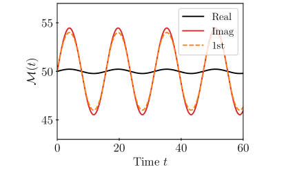
While the results in Eqs. (27) and (28) indicate that this is a periodic oscillation with period , the pattern is not so explicit. Nevertheless, for a finite system size , we introduce the center of the wave packet:
| (29) |
The numerical results of for different values of are presented in Fig. 3. The figure shows that the center of the wave packet undergoes the BO over time, and the amplitude is on the order of magnitude for an imaginary . However, for a real , the center of the wave packet remains near the initial position . This is opposite to that in the previous Gaussian initial state.
IV Numerical simulations
Thus far, we have analyzed the time evolutions for three different initial excitations in the framework of the low-energy effective Hamiltonian in Eq (7). It is worth noting that in the non-Hermitian system, the magnetic BO is absent for an initial Gaussian state but emerges for an initial Bessel state, which is distinct from the Hermitian system. In this section, we present the numerical simulations of the time evolutions for the three initial states under the original Hamiltonian in Eq. (1), in order to verify the previous analyses.
The initial states are taken as
| (30) |
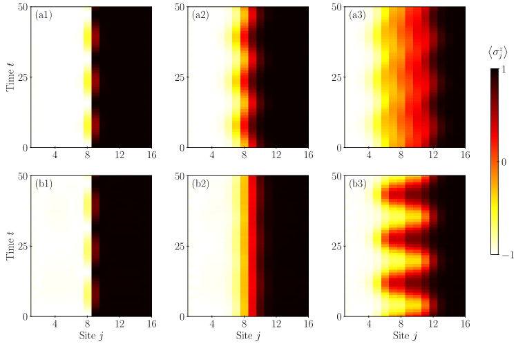
with , and , representing the Kronecker delta state, Gaussian state, and Bessel state, respectively, which are investigated in the previous section. The centers of these localized initial states are all set as , i.e., at the middle of the chain, to avoid boundary effects. The evolved state is calculated under the spin Hamiltonian in Eq. (1) using the fourth-order Runge-Kutta method with time steps of length , with a total accumulated error on the order of . The evolved state is normalized after each time step, and the local spin expectation value is computed after each 100 time steps. The results are presented in Fig. 4, and other parameters of the system and initial states are presented in the caption.
The boundary of and is the position of the magnetic domain wall. For the Hermitian spin chain, Figs. 4(a1)-(a3) show that the dynamics are magnetic Bloch breathing, BO, and stationary modes for the Kronecker delta, Gaussian, and Bessel initial states, respectively. With the same initial states, for the non-Hermitian spin chain, the results in Figs. 4(b1)-(b3) indicate that the dynamics are magnetic Bloch breathing, stationary, and BO modes, respectively. For the latter two initial states, the corresponding BOs exhibit totally different patterns for the same initial states in the two different systems. These numerical results are in accordance with the analyses in the previous section.
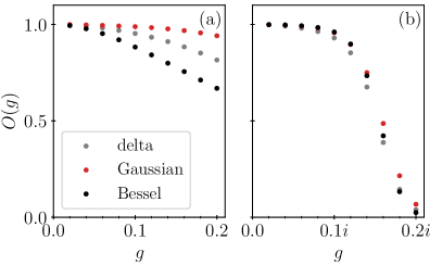
In order to further estimate the validity of perturbative solutions presented in the previous section, we compare the numerical evolved states with perturbative solutions by the overlap
| (31) |
at instant , where and denote the normalized numerical and analytical evolved states, respectively. The perturbative solutions for three initial states are taken as the form of Eq. (16) with being Eqs. (III.1), (23) and (27), respectively. In Fig. 5, we presented the numerical results of overlap at instant as a function of real and imaginary . It indicates that for both cases, the perturbative solutions are in good agreement with the exact numerical results in a small , while for imaginary the overlap drops sharply when due to the symmetry breaking of that is not captured by the effective Hamiltonian .
V Summary
In summary, we demonstrate the existence of the magnetic BOs in a non-Hermitian quantum Ising chain. It is shown that in the small-field region, the low-energy dynamics of the magnetic domain walls are captured by a single-particle effective Hamiltonian, with the transverse field acting as a hopping coefficient for the magnetic domain wall and the strength of the longitudinal field playing the role of a skew potential. For real and imaginary transverse fields, the eigenstates of the effective Hamiltonian are both localized states with equally spaced energy levels, forming the WS ladders. Analytical and numerical calculations of the time evolution for the non-Hermitian quantum Ising chain show the following.
(i) The dynamics of the Kronecker delta initial state follow a breathing mode.
(ii) The Gaussian state remains stationary, which is different from the oscillation of the domain wall in a Hermitian quantum Ising chain.
(iii) For the Bessel initial state, the oscillation mode appears, and the amplitude can be modulated by the strength of the imaginary transverse field and the localization length of the initial state.
The validity of perturbative solutions is estimated by comparing them with numerical results. Our results reveal the mechanism of magnetic BOs in the non-Hermitian quantum spin chain and pave the way for future research on BOs in other quantum systems.
Acknowledgements.
This work was supported by the National Natural Science Foundation of China (under Grant No. 12374461).References
- Bloch [1929] F. Bloch, Über die quantenmechanik der elektronen in kristallgittern, Z. Phys. 52, 555 (1929).
- Zener [1934] C. Zener, A theory of the electrical breakdown of solid dielectrics, Proc. R. Soc. London, Ser. A 145, 523 (1934).
- Wannier [1960] G. H. Wannier, Wave functions and effective Hamiltonian for Bloch electrons in an electric field, Phys. Rev. 117, 432 (1960).
- Waschke et al. [1993] C. Waschke, H. G. Roskos, R. Schwedler, K. Leo, H. Kurz, and K. Köhler, Coherent submillimeter-wave emission from Bloch oscillations in a semiconductor superlattice, Phys. Rev. Lett. 70, 3319 (1993).
- Ben Dahan et al. [1996] M. Ben Dahan, E. Peik, J. Reichel, Y. Castin, and C. Salomon, Bloch oscillations of atoms in an optical potential, Phys. Rev. Lett. 76, 4508 (1996).
- Wilkinson et al. [1996] S. R. Wilkinson, C. F. Bharucha, K. W. Madison, Q. Niu, and M. G. Raizen, Observation of atomic Wannier-Stark ladders in an accelerating optical potential, Phys. Rev. Lett. 76, 4512 (1996).
- Anderson and Kasevich [1998] B. P. Anderson and M. A. Kasevich, Macroscopic quantum interference from atomic tunnel arrays, Science 282, 1686 (1998).
- Morsch et al. [2001] O. Morsch, J. H. Müller, M. Cristiani, D. Ciampini, and E. Arimondo, Bloch oscillations and mean-field effects of Bose-Einstein condensates in 1D optical lattices, Phys. Rev. Lett. 87, 140402 (2001).
- Morandotti et al. [1999] R. Morandotti, U. Peschel, J. S. Aitchison, H. S. Eisenberg, and Y. Silberberg, Experimental observation of linear and nonlinear optical Bloch oscillations, Phys. Rev. Lett. 83, 4756 (1999).
- Sanchis-Alepuz et al. [2007] H. Sanchis-Alepuz, Y. A. Kosevich, and J. Sánchez-Dehesa, Acoustic analogue of electronic Bloch oscillations and resonant Zener tunneling in ultrasonic superlattices, Phys. Rev. Lett. 98, 134301 (2007).
- Meinert et al. [2017] F. Meinert, M. Knap, E. Kirilov, K. Jag-Lauber, M. B. Zvonarev, E. Demler, and H.-C. Nägerl, Bloch oscillations in the absence of a lattice, Science 356, 945 (2017).
- Zhang et al. [2022] W. Zhang, H. Yuan, H. Wang, F. Di, N. Sun, X. Zheng, H. Sun, and X. Zhang, Observation of Bloch oscillations dominated by effective anyonic particle statistics, Nat. Commun. 13, 2392 (2022).
- Hansen et al. [2022] U. B. Hansen, O. F. Syljuåsen, J. Jensen, T. K. Schäffer, C. R. Andersen, M. Boehm, J. A. Rodriguez-Rivera, N. B. Christensen, and K. Lefmann, Magnetic Bloch oscillations and domain wall dynamics in a near-Ising ferromagnetic chain, Nat. Commun. 13, 2547 (2022).
- Kyriakidis and Loss [1998] J. Kyriakidis and D. Loss, Bloch oscillations of magnetic solitons in anisotropic spin- chains, Phys. Rev. B 58, 5568 (1998).
- Sudzius et al. [1998] M. Sudzius, V. G. Lyssenko, F. Löser, K. Leo, M. M. Dignam, and K. Köhler, Optical control of Bloch-oscillation amplitudes: From harmonic spatial motion to breathing modes, Phys. Rev. B 57, R12693 (1998).
- Kosevich [2001] Y. A. Kosevich, Anomalous Hall velocity, transient weak supercurrent, and coherent Meissner effect in semiconductor superlattices, Phys. Rev. B 63, 205313 (2001).
- Cai et al. [2011] Z. Cai, L. Wang, X. C. Xie, U. Schollwöck, X. R. Wang, M. Di Ventra, and Y. Wang, Quantum spinon oscillations in a finite one-dimensional transverse Ising model, Phys. Rev. B 83, 155119 (2011).
- Shinkevich and Syljuåsen [2012] S. Shinkevich and O. F. Syljuåsen, Spectral signatures of magnetic Bloch oscillations in one-dimensional easy-axis ferromagnets, Phys. Rev. B 85, 104408 (2012).
- Kosevich and Gann [2013] Y. A. Kosevich and V. V. Gann, Magnon localization and Bloch oscillations in finite Heisenberg spin chains in an inhomogeneous magnetic field, J. Phys.: Condens.Matter 25, 246002 (2013).
- Shinkevich and Syljuåsen [2013] S. Shinkevich and O. F. Syljuåsen, Numerical simulations of laser-excited magnetic Bloch oscillations, Phys. Rev. B 87, 060401 (2013).
- Syljuåsen [2015] O. F. Syljuåsen, Dynamical structure factor of magnetic Bloch oscillations at finite temperatures, Eur. Phys. J. B 88, 1 (2015).
- Longhi [2009a] S. Longhi, Bloch oscillations in complex crystals with symmetry, Phys. Rev. Lett. 103, 123601 (2009a).
- Jin and Song [2010] L. Jin and Z. Song, Physics counterpart of the non-Hermitian tight-binding chain, Phys. Rev. A 81, 032109 (2010).
- Lee and Chan [2014] T. E. Lee and C.-K. Chan, Heralded magnetism in non-Hermitian atomic systems, Phys. Rev. X 4, 041001 (2014).
- Jin [2017] L. Jin, Topological phases and edge states in a non-Hermitian trimerized optical lattice, Phys. Rev. A 96, 032103 (2017).
- Qin et al. [2020] C. Qin, B. Wang, Z. J. Wong, S. Longhi, and P. Lu, Discrete diffraction and Bloch oscillations in non-Hermitian frequency lattices induced by complex photonic gauge fields, Phys. Rev. B 101, 064303 (2020).
- Ashida et al. [2020] Y. Ashida, Z. Gong, and M. Ueda, Non-Hermitian physics, Adv. Phys. 69, 249 (2020).
- Jin and Song [2021] L. Jin and Z. Song, Symmetry-protected scattering in non-Hermitian linear systems, Chin. Phys. Lett. 38, 024202 (2021).
- Zhang et al. [2021] W. Zhang, X. Ouyang, X. Huang, X. Wang, H. Zhang, Y. Yu, X. Chang, Y. Liu, D.-L. Deng, and L.-M. Duan, Observation of non-Hermitian topology with nonunitary dynamics of solid-state spins, Phys. Rev. Lett. 127, 090501 (2021).
- Rohn et al. [2023] J. Rohn, K. P. Schmidt, and C. Genes, Classical phase synchronization in dissipative non-Hermitian coupled systems, Phys. Rev. A 108, 023721 (2023).
- Liang et al. [2023] C. Liang, Y. Tang, A.-N. Xu, and Y.-C. Liu, Observation of exceptional points in thermal atomic ensembles, Phys. Rev. Lett. 130, 263601 (2023).
- Xu and Jin [2023] H. S. Xu and L. Jin, Pseudo-Hermiticity protects the energy-difference conservation in the scattering, Phys. Rev. Res. 5, L042005 (2023).
- Xu et al. [2023] H. S. Xu, L. C. Xie, and L. Jin, High-order spectral singularity, Phys. Rev. A 107, 062209 (2023).
- Longhi [2009b] S. Longhi, Dynamic localization and transport in complex crystals, Phys. Rev. B 80, 235102 (2009b).
- Ramya Parkavi et al. [2021] J. Ramya Parkavi, V. K. Chandrasekar, and M. Lakshmanan, Stable Bloch oscillations and Landau-Zener tunneling in a non-Hermitian -symmetric flat-band lattice, Phys. Rev. A 103, 023721 (2021).
- Longhi [2014] S. Longhi, Exceptional points and Bloch oscillations in non-Hermitian lattices with unidirectional hopping, Europhys. Lett. 106, 34001 (2014).
- Longhi [2015] S. Longhi, Bloch oscillations in non-Hermitian lattices with trajectories in the complex plane, Phys. Rev. A 92, 042116 (2015).
- Graefe et al. [2016] E.-M. Graefe, H. Korsch, and A. Rush, Quasiclassical analysis of Bloch oscillations in non-Hermitian tight-binding lattices, New J. Phys. 18, 075009 (2016).
- Naghiloo et al. [2019] M. Naghiloo, M. Abbasi, Y. N. Joglekar, and K. Murch, Quantum state tomography across the exceptional point in a single dissipative qubit, Nat. Phys. 15, 1232 (2019).
- Partanen et al. [2019] M. Partanen, J. Goetz, K. Y. Tan, K. Kohvakka, V. Sevriuk, R. E. Lake, R. Kokkoniemi, J. Ikonen, D. Hazra, A. Mäkinen, E. Hyyppä, L. Grönberg, V. Vesterinen, M. Silveri, and M. Möttönen, Exceptional points in tunable superconducting resonators, Phys. Rev. B 100, 134505 (2019).
- Wu et al. [2019] Y. Wu, W. Liu, J. Geng, X. Song, X. Ye, C.-K. Duan, X. Rong, and J. Du, Observation of parity-time symmetry breaking in a single-spin system, Science 364, 878 (2019).
- Li et al. [2019] J. Li, A. K. Harter, J. Liu, L. de Melo, Y. N. Joglekar, and L. Luo, Observation of parity-time symmetry breaking transitions in a dissipative Floquet system of ultracold atoms, Nat. Commun. 10, 855 (2019).
- Ren et al. [2022] Z. Ren, D. Liu, E. Zhao, C. He, K. K. Pak, J. Li, and G.-B. Jo, Chiral control of quantum states in non-Hermitian spin–orbit-coupled fermions, Nat. Phys. 18, 385 (2022).
- Zhang and Song [2020] K. L. Zhang and Z. Song, Ising chain with topological degeneracy induced by dissipation, Phys. Rev. B 101, 245152 (2020).
- Liu et al. [2021] Y.-G. Liu, L. Xu, and Z. Li, Quantum phase transition in a non-Hermitian XY spin chain with global complex transverse field, J. Phys.: Condens.Matter 33, 295401 (2021).
- Zhang and Song [2021] K. L. Zhang and Z. Song, Quantum phase transition in a quantum Ising chain at nonzero temperatures, Phys. Rev. Lett. 126, 116401 (2021).
- Lenke et al. [2021] L. Lenke, M. Mühlhauser, and K. P. Schmidt, High-order series expansion of non-Hermitian quantum spin models, Phys. Rev. B 104, 195137 (2021).
- Matsumoto et al. [2022] N. Matsumoto, M. Nakagawa, and M. Ueda, Embedding the Yang-Lee quantum criticality in open quantum systems, Phys. Rev. Res. 4, 033250 (2022).
- Guo et al. [2022] Z.-X. Guo, X.-J. Yu, X.-D. Hu, and Z. Li, Emergent phase transitions in a cluster Ising model with dissipation, Phys. Rev. A 105, 053311 (2022).
- Sun et al. [2022] G. Sun, J.-C. Tang, and S.-P. Kou, Biorthogonal quantum criticality in non-Hermitian many-body systems, Front. Phys. 17, 1 (2022).
- Gao et al. [2023] H. Gao, K. Wang, L. Xiao, M. Nakagawa, N. Matsumoto, D. Qu, H. Lin, M. Ueda, and P. Xue, Experimental observation of the Yang-Lee quantum criticality in open systems, arXiv:2312.01706 (2023).
- Lu et al. [2023] C.-Z. Lu, X. Deng, S.-P. Kou, and G. Sun, Unconventional many-body phase transitions in a non-Hermitian Ising chain, arXiv:2311.11251 (2023).
- Lenke et al. [2023] L. Lenke, A. Schellenberger, and K. P. Schmidt, Series expansions in closed and open quantum many-body systems with multiple quasiparticle types, Phys. Rev. A 108, 013323 (2023).
- Yang and Lee [1952] C. N. Yang and T. D. Lee, Statistical theory of equations of state and phase transitions. I. theory of condensation, Phys. Rev. 87, 404 (1952).
- Lee and Yang [1952] T. D. Lee and C. N. Yang, Statistical theory of equations of state and phase transitions. II. lattice gas and Ising model, Phys. Rev. 87, 410 (1952).
- Von Gehlen [1991] G. Von Gehlen, Critical and off-critical conformal analysis of the Ising quantum chain in an imaginary field, Journal of Physics A: Mathematical and General 24, 5371 (1991).
- Castro-Alvaredo and Fring [2009] O. A. Castro-Alvaredo and A. Fring, A spin chain model with non-Hermitian interaction: the Ising quantum spin chain in an imaginary field, J. Phys. A: Math. Theor. 42, 465211 (2009).
- Ananikian and Kenna [2015] N. Ananikian and R. Kenna, Imaginary magnetic fields in the real world, Physics 8, 2 (2015).
- Peng et al. [2015] X. Peng, H. Zhou, B.-B. Wei, J. Cui, J. Du, and R.-B. Liu, Experimental observation of Lee-Yang zeros, Phys. Rev. Lett. 114, 010601 (2015).
- Sanno et al. [2022] T. Sanno, M. G. Yamada, T. Mizushima, and S. Fujimoto, Engineering Yang-Lee anyons via Majorana bound states, Phys. Rev. B 106, 174517 (2022).
- Pfeuty [1970] P. Pfeuty, The one-dimensional Ising model with a transverse field, Ann. Phys. 57, 79 (1970).
- Daley [2014] A. J. Daley, Quantum trajectories and open many-body quantum systems, Adv. Phys. 63, 77 (2014).
- Biella and Schiró [2021] A. Biella and M. Schiró, Many-body quantum zeno effect and measurement-induced subradiance transition, Quantum 5, 528 (2021).
- Turkeshi and Schiró [2023] X. Turkeshi and M. Schiró, Entanglement and correlation spreading in non-Hermitian spin chains, Phys. Rev. B 107, L020403 (2023).
- Bender and Boettcher [1998] C. M. Bender and S. Boettcher, Real spectra in non-Hermitian Hamiltonians having symmetry, Phys. Rev. Lett. 80, 5243 (1998).
- Bender et al. [1999] C. M. Bender, S. Boettcher, and P. N. Meisinger, -symmetric quantum mechanics, J. Math. Phys. 40, 2201 (1999).
- Mostafazadeh [2002] A. Mostafazadeh, Pseudo-Hermiticity versus PT symmetry: the necessary condition for the reality of the spectrum of a non-Hermitian Hamiltonian, J. Math. Phys. 43, 205 (2002).
- Sanz et al. [2016] M. Sanz, E. Solano, and Í. L. Egusquiza, Beyond adiabatic elimination: Effective Hamiltonians and singular perturbation, in Applications+ Practical Conceptualization+ Mathematics= fruitful Innovation: Proceedings of the Forum of Mathematics for Industry 2014 (Springer, 2016) pp. 127–142.
- Fukuyama et al. [1973] H. Fukuyama, R. A. Bari, and H. C. Fogedby, Tightly bound electrons in a uniform electric field, Phys. Rev. B 8, 5579 (1973).
- Krimer et al. [2009] D. O. Krimer, R. Khomeriki, and S. Flach, Delocalization and spreading in a nonlinear Stark ladder, Phys. Rev. E 80, 036201 (2009).
- Abramowitz and Stegun [1968] M. Abramowitz and I. A. Stegun, Handbook of mathematical functions with formulas, graphs, and mathematical tables, Vol. 55 (US Government printing office, 1968).
- Holthaus and Hone [1996] M. Holthaus and D. W. Hone, Localization effects in ac-driven tight-binding lattices, Philos. Mag. B 74, 105 (1996).
- Truesdell [1950] C. Truesdell, On the addition and multiplication theorems for special functions, Proc. Natl. Acad. Sci. 36, 752 (1950).