MADLens, a python package for fast and differentiable non-Gaussian lensing simulations
Abstract
We present MADLens a python package for producing non-Gaussian lensing convergence maps at arbitrary source redshifts with unprecedented precision. MADLens is designed to achieve high accuracy while keeping computational costs as low as possible. A MADLens simulation with only particles produces convergence maps whose power agree with theoretical lensing power spectra up to within the accuracy limits of HaloFit. This is made possible by a combination of a highly parallelizable particle-mesh algorithm, a sub-evolution scheme in the lensing projection, and a machine-learning inspired sharpening step. Further, MADLens is fully differentiable with respect to the initial conditions of the underlying particle-mesh simulations and a number of cosmological parameters. These properties allow MADLens to be used as a forward model in Bayesian inference algorithms that require optimization or derivative-aided sampling. Another use case for MADLens is the production of large, high resolution simulation sets as they are required for training novel deep-learning-based lensing analysis tools. We make the MADLens package publicly available under a Creative Commons License \faGithub.
keywords:
gravitational lensing , cosmological parameters , methods: N-body simulations1 Introduction
Measurements of the weak cosmic shear signal will be among the major experimental drivers for advancing cosmology in the next decade. Next generation surveys such as LSST (LSST Science Collaboration et al., 2009), the Roman Space Telescope (Spergel et al., 2015) and the EUCLID satellite (Euclid Collaboration et al., 2020) will provide an unprecedented amount of high resolution weak cosmic shear data, which creates a demand for novel data analysis and modeling techniques. The weak cosmic shear signal is sensitive to the evolution of matter clustering over several orders of scales, ranging from well within the linear to the highly non-linear regime. Tomographic lensing measurements are sensitive to the total matter content, , the amplitude of clustering, , and the time evolution of clustering, which allows to constrain dark energy (Hu, 2002; Huterer, 2002; Song and Knox, 2004) and the sum of neutrino masses. Weak cosmic shear measurements can further be used to test general relativity (Heavens et al., 2007; Schmidt, 2008; Harnois-Déraps et al., 2015).
Traditional lensing analyses mostly rely on two-point statistics or related observables (Kitching et al., 2011; Heymans et al., 2013; Kitching et al., 2014; Alsing et al., 2016; Hildebrandt et al., 2017; DES Collaboration et al., 2018; Taylor et al., 2019; Hikage et al., 2019) to extract cosmological information. However, since the lensing convergence field is inherently and significantly non-Gaussian, two-point statistics do not exploit its full information content. In fact, a long list of studies have shown that non-Gaussian summary statistics, such as higher order correlation functions (Pen et al., 2003; Takada and Jain, 2003; Jarvis et al., 2004; Semboloni et al., 2011; Fu et al., 2014; Coulton et al., 2019) or peak statistics (Jain and Van Waerbeke, 2000; Dietrich and Hartlap, 2010; Maturi et al., 2011; Marian et al., 2012; Pires et al., 2012; Petri et al., 2013; Cardone et al., 2013; Lin and Kilbinger, 2015; Liu et al., 2015a, b; Kacprzak et al., 2016; Peel et al., 2017; Li et al., 2019) can break parameter degeneracies that cumber power spectrum analyses and lead to significantly tighter constraints. While inference from these summaries offers improvements over power spectra analyses, their choice is somewhat ad hoc and the question of how to best extract cosmological information from non-Gaussian lensing scales is still an active field of research.
A number of works have recently suggested machine-learning tools for identifying informative summaries (Gupta et al., 2018; Ribli et al., 2019) and even successfully applied them to real data (Fluri et al., 2019). Machine learning methods require a large amount of training data. If applied correctly, these methods learn which features in the lensing map are most informative about cosmological parameters. A recent study finds that these models are mostly sensitive to extreme values in the lensing field (Zorrilla Matilla et al., 2020). This underlines the importance of training data that accurately mimics real cosmic shear data and its dependence on cosmological parameters down to very small scales.
Another approach, and in principle the optimal one, is to build a differentiable non-linear data model that starts from the Gaussian initial conditions and forward models them accurately to the measured lensing signal. This forward model is used to model the posterior of the parameters of interest (these can be cosmological parameters, the modes of the initial field or the bandpowers of the initial power spectrum). Analyzing this posterior generally relies on powerful sampling or optimization schemes, which in turn require many model evaluations and the derivatives of the model with respect to the parameters of interest. Forward-model based inference schemes have been developed for a range of of observables in cosmology (Seljak, 1998; Seljak et al., 2017; Jasche and Kitaura, 2010; Jasche and Wandelt, 2013) including weak cosmic shear (Böhm et al., 2017; Porqueres et al., 2020).
All of these new avenues for lensing analyses create the need for fast and differentiable simulations of the lensing field that at the same time accurately capture the nonlinear features of that field.
Realistic lensing simulations are challenging because a range of scales in the three dimensional matter distribution contribute to a single angular scale in the lensing field making even intermediate lensing scales sensitive to the non-linearity of structure formation on small scales (Jain and Seljak, 1997). Accurate lensing simulations rely on lightcones constructed from high resolution N-body simulations. These N-body simulations must accurately resolve small scales, but must at the same time be large enough to produce lensing maps with an extent of several degrees.
A number of recent works have studied the applicability of deep generative models, in particular generative adversarial networks (GANs) for producing accurate lensing convergence maps at low computational costs (Mustafa et al., 2019; Perraudin et al., 2020). These models do not aim at simulating the underlying physics, but are trained to mimic the training data to a degree where their output becomes indistinguishable from the training data for a neural network. While these early studies look promising, future research will have to show that these models indeed learn the correct data distribution or that using their outputs for inference leads to unbiased parameter posteriors. Another, more safeguard approach is to use machine-learning inspired techniques to boost the accuracy of low resolution N-body simulations (Dai et al., 2020; Dai and Seljak, 2020) and to construct lightcones from those. This is the avenue we have chosen in this work to create high resolution lensing simulations from approximate N-body solvers.
In this publication we describe a new, weak gravitational lensing package, MADLens. MADLens is a python package that allows to compute fully nonlinear lensing convergence maps at different source redshifts and low computational cost while accurately modeling the non-Gaussianity of the field down to scales of several tens of arcseconds. MADLens is built on top of a particle-mesh solver that evolves an initial linear density field into non-linear late time density fields. It provides derivatives with respect to the initial conditions of the particle-mesh simulation and a number of cosmological parameters through automated differentiation. MADLens fills the gap in the accuracy-speed space between computationally expensive, high accuracy lensing simulations and fast approximate simulations. In particular, MADLens correctly captures scales down to at a field of view (FOV) of with percent level precision at a runtime of 30 seconds on 32 processes. MADLens can be run at different levels of resolution and approximations, allowing the user to choose the speed to accuracy trade-off that is optimal for their application.
We begin this paper with a brief introduction of the cosmological-scale weak lensing formalism and our notation in Section 2. This is followed by a in depth discussion of the package design in Section 3. We demonstrate the packages abilities in a number of tests in Section 4 and conclude with a summary and outlook in Section 5. A provides details on the novel feature of differentiability with respect to cosmological parameters.
2 Weak Gravitational Lensing, Notation and Conventions
Weak gravitational lensing observations provide insight into the projected matter density distribution between an observer and a source through correlated image distortions. Here, we provide a brief overview and define our usage of the lensing kernel, lensing convergence, and power spectrum of cosmic shear used throughout MADLens (for a detailed discussion of weak gravitational lensing and especially cosmic shear, see Bartelmann and Maturi (2017); Kilbinger (2015); Bartelmann and Schneider (2001)).
The image of a source galaxy at a comoving distance is distorted along the line of sight by some lensing potential . The potential of an extended lens under the Born approximation representing all density fluctuations along a line of sight at some angular position can be found by integrating individual Weyl potentials up to the comoving distance of the galaxy,
| (1) |
where is the angular perpendicular component of the potential and is the parallel component. The lensing deflection and convergence are defined as,
| (2) |
where the derivatives are taken with respect to . Using the Poisson equation and neglecting derivative along the line-of-sight direction, the lensing convergence can be rewritten as,
| (3) | ||||
| (4) |
where represents the density contrast from the mean density, is the Hubble parameter and is the lensing kernel describing the projection of sources selected by the redshift selection function . MADLens evaluates the integral in Eq. 3 numerically. The most commonly used summary statistic in lensing analyses that can also be computed analytically is the power spectrum. To compute the convergence power spectrum we use Limber’s approximation and the flat sky approximation which are both valid on intermediate and small scales,
| (5) |
Since the lensing power spectrum is very sensitive to non-linear corrections to the matter power spectrum, we use HaloFit (Takahashi et al., 2012) to model throughout this paper.
| Parameter | Description | Typical Value(s) |
|---|---|---|
| BoxSize | side length of the simulation box | 128-1024 Mpc/h |
| Nmesh | resolution of the particle-mesh simulation | |
| B | force resolution factor | |
| Nsteps | number of steps in the FastPM simulation | |
| N_maps | number of output maps | |
| Nmesh2D | resolution of the convergence map | |
| BoxSize2D | size of the convergence map in degrees | |
| zs_source | list of source redshifts | |
| Omega_m | total matter density | |
| sigma_8 | amplitude of matter fluctuations | |
| PGD | whether to use PGD enhancement or not | True/False |
| interpolation | whether to use the sub-evolution scheme | True/False |
3 MADLens package design
The MADLens package is based on FastPM (Feng et al., 2016), a highly scalable particle-mesh solver, that evolves particle positions through a kick and drift scheme enforcing correct linear displacement in each step. FastPM has been implemented in C and Python and two versions of FastPM support automatic differentiation, including the MPI based version used in this work, and the recently published FlowPM (Modi et al., 2020) package, which is based on TensorFlow. A FastPM particle-mesh simulation requires the choice of a particle-mesh resolution, equivalent to the number of particles in the simulation, the force resolution, the resolution of the grid onto which the particles are painted to compute the forces, the box size of the simulation and the number of steps in which the particle positions are evolved. The initial conditions and particle evolution depend on the cosmological parameters and .
MADLens runs a FastPM simulation. As the simulation evolves, MADLens projects the particles in the simulation weighted by the lensing kernel at each simulation step to 2D meshes at the desired source redshifts. The field of view, i.e. the size of the convergence map, and its resolution can be set by the user given the simulation box covers the entire field of view at the most distant source redshift. Each FastPM step evolves particles in redshift steps, . MADLens constructs the lightcone by translating these redshifts into distances and projecting particles at the correct evolution step corresponding to that distance onto the convergence map. If the distance between two simulation steps is larger than the extent of the box, the box is replicated at the same redshift as often as is needed to fill the entire extent. In order to avoid spurious correlations, the simulations box is rotated before being repeated. In these techniques, MADLens is constructed similarly to other lightcone packages. We provide an overview of all MADLens parameters that can be set by the user in table 1.
To reach extraordinary accuracy at low computational costs, MADLens employs two special techniques:
-
1.
Particle Gradient Descent (PGD) (Dai et al., 2018) is an additional particle evolution step that corrects for the difference between particle distributions in a low resolution simulation and a high resolution simulation. The correction is applied after each simulation step. PGD introduces 5 additional nuisance parameters, which are fitted on training simulations. PGD allows simulations to run at lower resolution while still obtaining results that are comparable and highly correlated with a high resolution simulation.
-
2.
A sub-evolution step allows for a massive reduction of the number of simulations steps. When using sub-evolution, particles are evolved according to the redshift of their position within the simulation box before projection, rather than by the redshift of the FastPM step.
Finally, MADLens is made differentiable through numerically accurate tape-based automatic differentiation. Specifically it uses the Virtual Machine Automated Differentiation package (VMAD). VMAD builds a graph that is traversed for the model evaluation, during which all operations are recorded on a sequential tape. Gradient graphs generated from the tape are used to compute Jacobian vector products () and vector Jacobian products (, commonly referred to as back-propagation). MADLens is made available in two variants. In its main version it is built to provide differentiability with respect to the initial, Gaussian modes of the simulation. A second package version, that is included in this release, adds differentiability with respect to the cosmological parameters, and . Differentiability with respect to the PGD paramaters (, , , ) will be included in a future release.
4 Results
We analyze the performance of MADLens, the PGD enhancement, the sub-evolution scheme and computation times as well as the accuracy of the gradient computation. Testing the accuracy of MADLens output is challenging, because of the lack of a ground truth. We will use theoretical power spectra based on Halofit matter power spectra and high resolution runs for comparison. These can serve as a reasonable baseline, but as should become evident from our analysis, should not be mistaken for the ground truth.

In Figure 1 we show an example of a convergence map produced with MADLens. The non-Gaussian structure is clearly visible by eye and also evident in the corresponding histogram in Figure 2. The map resolves sub arcmin scales and extends over more than on the sky showing that MADLens overcomes one of the key challenges in lensing simulations: the accurate modeling of both large and small scales.

We compare the histogram of pixel values in Figure 2 with a log-normal distribution. Log-normal distributions have been used in the past to model lensing PDFs, but are not strictly theoretically motivated. The log-normal fit captures the rough shape of the distribution, but underestimates the probability of high values and overestimates the probability of low values.
4.1 Accuracy

In Figure 3 we compare the power spectra measured from MADLens outputs at different source redshifts with the analytical model of Eq. 5 based on a HaloFit matter power spectrum. For this comparison we average the power spectra of five simulations to reduce the variance. Overall we find that the MADLens power spectra trace the theoretical predictions well within up to scales of a few thousand. At very small scales shot noise starts to contribute significantly to the power. To put the importance of this shot noise into perspective we further plot the experimental noise level expected in a typical future experiment, such as LSST, and find that the shot noise is subdominant to the expected noise levels in real data.

Figure 4 delves further into the comparison with theoretical power spectrum and quantification of the shot noise. We translate the HaloFit accuracy ( for at and for at ) into accuracy in the lensing power spectrum and show these intervals as gray bands. The MADLens power spectrum lies well within these bands up to wavenumbers of a few thousand, where it becomes dominated by shot noise. We estimate the shot noise level by running a number of MADlens simulations with random particle positions (dark gray line) and subtract the result from the MADLens power spectrum (dark blue). The result lies within the HaloFit accuracy up to .

Figure 5 shows that the PGD enhancement allows to reach these high accuracies at much lower computational cost than conventional lensing simulations. We compare the output of MADLens simulations at a resolution of 1 particle per Mpc/h cubed to a conventional simulation (MADLens without PGD) with an eight times higher resolution. The higher resolution simulation not only requires about eight times more memory, but also takes more than twice as long. The high resolution run is of comparable resolution to other state-of-the-art lensing simulations which have been used for cosmological parameter inference studies (Liu et al., 2018), but the lower resolution MADLens simulation traces the theoretical convergence power spectrum up to much higher wavenumbers.

In Figure 6 we show cross correlations defined by
| (6) |
where is the high resolution run without PGD enhancement, and are lower resolution MADLens outputs that have either been produced with or without PGD enhancement. As expected, the PGD enhanced lower resolution map shows higher correlation (dark blue) with the high resolution run than the one without enhancement (light blue) on intermediate scales. The results of this cross correlation analysis must be taken with a grain of salt: since the high resolution run is suffering from a significant lack of power on small scales, this could also be an indication of inaccurate particle positions. A lower cross correlation on small scales simply states that the simulations differ significantly, but does not show which one is more correct.

The accuracy of MADLens is further boosted by a sub-evolution projection scheme, where particles are moved to the position corresponding to their actual distance to the observer before being projected on the lensing map. We illustrate the efficacy of this scheme in Figure 7. An 11-step simulation naturally overestimates the total lensing power (light blue). The sub-evolution scheme is able to correct for this overestimation up to scales (dark blue). In a 40 step simulation the discrepancy between actual particle positions and their true evolution stage is smaller (light red), however, even the accuracy of a 40 step simulation can be enhanced by the sub-evolution scheme (dark red).

The MADLens derivatives have been thoroughly tested and verified with VMAD built-in test functions. Here we show that the derivatives are accurate by means of a single example: we build a finite difference test by slightly changing a single pixel value in the initial field. We then take the difference of the output maps generated from runs with slightly different values in this initial pixel and compare it with the output of the Jacobian-vector-product (Jvp), where the vector encapsulates the change in the initial field. If the Jvp vector product is correct, the result should agree with the difference of the output maps. That this is indeed the case is shown in Figure 8. The first two panels show the Jvp and the finite difference result, respectively. They are indistinguishable by eye. The next panel shows the difference between the first two panels, revealing insignificant numerical inaccuracies, five magnitudes smaller than the signal. In the last panel we compare the outputs in terms of their histograms, finding again an excellent match.
4.2 Run times
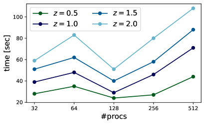
We conducted timing tests for MADLens on Intel® Xeon® Processors E5-2698 v3 (NERSC Cori Haswell nodes), and show results in Figures 9-12. A single MADLens simulation that achieves accuracies as shown in the last section takes of the order of 10-60 seconds on 32 processes. The scaling of the run-time with source redshift is roughly linear and reducing the number of particles by a factor of 8 reduces the run-time to about one third (Figure 9).


The computation time can be further reduced by paralellizing on up to processes, after which the communication overhead starts to dominate the time budget (Figure 10).
Reducing the number of FastPM steps leads to significant savings in run time as we demonstrate in Figure 11. A conventional lightcone code requires about 40 steps in order to reach percent accuracies in the lensing power spectrum up . With PGD enhancement and sub-evolution scheme, MADLens reaches percent accuracies up to with only 11 FastPM steps: a factor of 3 in time-savings.
The use of back-propagation to calculate the derivatives results in run times that are similar to the forward model. This is shown in Figure 12, where we find run times of 1.1-1.6 times the run time of the forward model for either Jvp and vJp.
5 Summary & Outlook
We have presented MADLens, a fully differentiable python package for producing non-Gaussian convergence maps of weak gravitational lensing on cosmological scales. MADLens reaches unprecedented accuracy even when compared to many non-differentiable lensing simulations, and operates at run times of the order of 2-20 below conventional N-body simulation based lightcone packages. These advancements are made possible by several features, including a machine learning inspired post processing step, that allows the N-body simulation to run at a lower resolution and with less steps without paying a significant penalty in accuracy. Taking the derivative through a MADLens simulation with respect to the initial modes of the N-body simulation and the two key cosmological parameters and is made possible through back-propagation. This means that evaluating the derivatives has comparable computational cost as the forward simulation. With these features MADLens constitutes a milestone towards the development of fully differentiable inference pipelines for weak cosmic shear. In the future MADLens will be integrated into the tensorflow-based FlowPM framework. Package updates will also feature differentiability with respect to nuisance parameters, such as the PGD parameters.
In the interest of scientific advancement and reproducibility, we make the MADLens package publicly available on github 111https://github.com/VMBoehm/MADLens.
Acknowledgements
This research used resources of the National Energy Research Scientific Computing Center (NERSC), a U.S. Department of Energy Office of Science User Facility operated under Contract No. DE-AC02-05CH11231. The authors thank Uros Seljak for useful discussions and feedback and Francois Lanusse for testing of the package and helpful feedback.
Appendix A Differentiability with respect to Cosmological Parameters
Since the forward model itself depends on cosmological parameters through the evolution of particle positions and the angular diameter distance which enters the lensing projection, an accurate inference algorithm needs to take these dependencies into account. To this end MADLens provides the additional functionality of derivatives with respect to the cosmological parameters and .
This novel application of derivatives requires both power spectra, particle evolution, and comoving distance calculations written as functions of cosmological parameters. The comoving distance calculation and derivative are trivial, and we use the standard definition (Peebles, 1993),
| (7) |
where . For a flat cosmology, we take and .

For the power spectrum that is applied to the initial density field, we use the transfer function defined in (Eisenstein and Hu, 1999) (EH-Transfer) with the inclusion of baryonic acoustic oscillation (BAO) wiggles. This is much simpler and computationally less involved than obtaining gradients of standard Boltzmann solvers with respect to cosmological parameters. Compared to the the matter power spectrum obtained from the Boltzmann package, CLASS (Blas et al., 2011), which is used for cosmological calculation throughout MADLens, we find discrepancies at a maximum of the level. We find that by using the EH-transfer, we slightly overestimate power on all scales with he largest discrepancies at those corresponding to BAO wiggles.
To show that this overestimation is within reason, we generate multiple convergence maps with both the CLASS and differentiable Eisenstein and Hu power spectrum. We show the absolute difference of the power spectra of these maps in Figure 13 and plot the cosmic variance for comparison. We find that the difference lies below the limit which we take to imply that our implementation of the EH-transfer function and power describes the initial spectrum well within the required accuracy.
The particle initial conditions and evolution, too, is dependant on the cosmology and we use a finite differencing scheme on the Lagrangian Perturbation Theory initial conditions, as well as the momentum and position updates in FastPM. This allows the computation of approximate, and accurate, derivatives for the initial conditions, kick, and drift factors without the need for analytical solutions to the derivatives with respect to . This method works by storing the finite difference of a function on the gradient tape, and caches the cosmology variables to avoid re-computation of the particle mesh. During forward propagation, the function is run as normal, and during back propagation two cached cosmology objects with perturbed parameter values are used to compute the finite difference. This scheme can be made applicable to any function which is not highly sensitive to parameters, and while we use the analytic solution for derivatives such as the EH-transfer function, it should be noted that it is feasible to apply the finite differencing method to linear power and cosmology methods from Boltzmann codes such as CLASS.
Similar to the finite difference test in section 4.1, we test the accuracy of the Jvp for . We add and subtract a small offset from (), compute convergence maps from both of these configurations and take their difference. We then compare this to the Jvp at the central value with a vector of to multiply the Jacobian. The resulting histograms are shown in Figure 14. The derivative of is in excellent agreement with the finite differencing result.
While only enters linearly, the model’s dependence on is more complicated. The derivative with respect to therefore requires a more in depth testing to ensure accurate derivatives are being taken. We test the Jacobian against finite differencing results for multiple modes individually. In Figure 15, we show the results of cross-correlating the finite difference results with the Jvp outputs and verify the accuracy of the automated derivative.
As a check for the vJp against , we construct a scalar by computing the finite differencing of the sum of the squared convergence maps and ensure that this value is equal to the vJp when the central convergence map is used as the vector in automated differentiation.
| (8) |
We find that the values agree at the level irrespective of the choice of .


References
- Alsing et al. (2016) Justin Alsing, Alan Heavens, and Andrew H. Jaffe et al. Hierarchical cosmic shear power spectrum inference. MNRAS, 455(4):4452–4466, February 2016. doi: 10.1093/mnras/stv2501.
- Bartelmann and Maturi (2017) Matthias Bartelmann and Matteo Maturi. Weak gravitational lensing. Scholarpedia, 12(1):32440, January 2017. doi: 10.4249/scholarpedia.32440.
- Bartelmann and Schneider (2001) Matthias Bartelmann and Peter Schneider. Weak gravitational lensing. Phys. Rept., 340:291–472, 2001. doi: 10.1016/S0370-1573(00)00082-X.
- Blas et al. (2011) Diego Blas, Julien Lesgourgues, and Thomas Tram. The Cosmic Linear Anisotropy Solving System (CLASS). Part II: Approximation schemes. J. Cosmology Astropart. Phys, 2011(7):034, July 2011. doi: 10.1088/1475-7516/2011/07/034.
- Böhm et al. (2017) Vanessa Böhm, Stefan Hilbert, and Maksim Greiner et al. Bayesian weak lensing tomography: Reconstructing the 3D large-scale distribution of matter with a lognormal prior. Phys. Rev. D, 96(12):123510, December 2017. doi: 10.1103/PhysRevD.96.123510.
- Cardone et al. (2013) V. F. Cardone, S. Camera, and R. Mainini et al. Weak lensing peak count as a probe of f(R) theories. MNRAS, 430(4):2896–2909, April 2013. doi: 10.1093/mnras/stt084.
- Coulton et al. (2019) William R. Coulton, Jia Liu, and Mathew S. Madhavacheril et al. Constraining neutrino mass with the tomographic weak lensing bispectrum. J. Cosmology Astropart. Phys, 2019(5):043, May 2019. doi: 10.1088/1475-7516/2019/05/043.
- Dai and Seljak (2020) Biwei Dai and Uros Seljak. Learning effective physical laws for generating cosmological hydrodynamics with Lagrangian Deep Learning. arXiv e-prints, art. arXiv:2010.02926, October 2020.
- Dai et al. (2018) Biwei Dai, Yu Feng, and Uroš Seljak. A gradient based method for modeling baryons and matter in halos of fast simulations. J. Cosmology Astropart. Phys, 2018(11):009, November 2018. doi: 10.1088/1475-7516/2018/11/009.
- Dai et al. (2020) Biwei Dai, Yu Feng, and Uroš Seljak et al. High mass and halo resolution from fast low resolution simulations. J. Cosmology Astropart. Phys, 2020(4):002, April 2020. doi: 10.1088/1475-7516/2020/04/002.
- DES Collaboration et al. (2018) DES Collaboration, M. A. Troxel, N. MacCrann, and J. Zuntz et al. Dark Energy Survey Year 1 results: Cosmological constraints from cosmic shear. Phys. Rev. D, 98(4):043528, August 2018. doi: 10.1103/PhysRevD.98.043528.
- Dietrich and Hartlap (2010) J. P. Dietrich and J. Hartlap. Cosmology with the shear-peak statistics. MNRAS, 402(2):1049–1058, February 2010. doi: 10.1111/j.1365-2966.2009.15948.x.
- Eisenstein and Hu (1999) Daniel J. Eisenstein and Wayne Hu. Power Spectra for Cold Dark Matter and Its Variants. ApJ, 511(1):5–15, January 1999. doi: 10.1086/306640.
- Euclid Collaboration et al. (2020) Euclid Collaboration, P. Paykari, T. Kitching, and H. Hoekstra et al. Euclid preparation. VI. Verifying the performance of cosmic shear experiments. A&A, 635:A139, March 2020. doi: 10.1051/0004-6361/201936980.
- Feng et al. (2016) Yu Feng, Man-Yat Chu, and Uroš Seljak et al. FASTPM: a new scheme for fast simulations of dark matter and haloes. MNRAS, 463(3):2273–2286, December 2016. doi: 10.1093/mnras/stw2123.
- Fluri et al. (2019) Janis Fluri, Tomasz Kacprzak, and Aurelien Lucchi et al. Cosmological constraints with deep learning from KiDS-450 weak lensing maps. Phys. Rev. D, 100(6):063514, September 2019. doi: 10.1103/PhysRevD.100.063514.
- Fu et al. (2014) Liping Fu, Martin Kilbinger, and Thomas Erben et al. CFHTLenS: cosmological constraints from a combination of cosmic shear two-point and three-point correlations. MNRAS, 441(3):2725–2743, July 2014. doi: 10.1093/mnras/stu754.
- Gupta et al. (2018) Arushi Gupta, José Manuel Zorrilla Matilla, and Daniel Hsu et al. Non-Gaussian information from weak lensing data via deep learning. Phys. Rev. D, 97(10):103515, May 2018. doi: 10.1103/PhysRevD.97.103515.
- Harnois-Déraps et al. (2015) J. Harnois-Déraps, D. Munshi, and P. Valageas et al. Testing modified gravity with cosmic shear. MNRAS, 454(3):2722–2735, December 2015. doi: 10.1093/mnras/stv2120.
- Heavens et al. (2007) A. F. Heavens, T. D. Kitching, and L. Verde. On model selection forecasting, dark energy and modified gravity. MNRAS, 380(3):1029–1035, September 2007. doi: 10.1111/j.1365-2966.2007.12134.x.
- Heymans et al. (2013) Catherine Heymans, Emma Grocutt, and Alan Heavens et al. CFHTLenS tomographic weak lensing cosmological parameter constraints: Mitigating the impact of intrinsic galaxy alignments. MNRAS, 432(3):2433–2453, July 2013. doi: 10.1093/mnras/stt601.
- Hikage et al. (2019) Chiaki Hikage, Masamune Oguri, and Takashi Hamana et al. Cosmology from cosmic shear power spectra with Subaru Hyper Suprime-Cam first-year data. PASJ, 71(2):43, April 2019. doi: 10.1093/pasj/psz010.
- Hildebrandt et al. (2017) H. Hildebrandt, M. Viola, and C. Heymans et al. KiDS-450: cosmological parameter constraints from tomographic weak gravitational lensing. MNRAS, 465(2):1454–1498, February 2017. doi: 10.1093/mnras/stw2805.
- Hu (2002) Wayne Hu. Dark energy and matter evolution from lensing tomography. Phys. Rev. D, 66(8):083515, October 2002. doi: 10.1103/PhysRevD.66.083515.
- Huterer (2002) Dragan Huterer. Weak lensing and dark energy. Phys. Rev. D, 65(6):063001, March 2002. doi: 10.1103/PhysRevD.65.063001.
- Jain and Seljak (1997) Bhuvnesh Jain and Uroš Seljak. Cosmological Model Predictions for Weak Lensing: Linear and Nonlinear Regimes. ApJ, 484(2):560–573, July 1997. doi: 10.1086/304372.
- Jain and Van Waerbeke (2000) Bhuvnesh Jain and Ludovic Van Waerbeke. Statistics of Dark Matter Halos from Gravitational Lensing. ApJ, 530(1):L1–L4, February 2000. doi: 10.1086/312480.
- Jarvis et al. (2004) M. Jarvis, G. Bernstein, and B. Jain. The skewness of the aperture mass statistic. MNRAS, 352(1):338–352, July 2004. doi: 10.1111/j.1365-2966.2004.07926.x.
- Jasche and Kitaura (2010) Jens Jasche and Francisco S. Kitaura. Fast Hamiltonian sampling for large-scale structure inference. MNRAS, 407(1):29–42, September 2010. doi: 10.1111/j.1365-2966.2010.16897.x.
- Jasche and Wandelt (2013) Jens Jasche and Benjamin D. Wandelt. Bayesian physical reconstruction of initial conditions from large-scale structure surveys. MNRAS, 432(2):894–913, June 2013. doi: 10.1093/mnras/stt449.
- Kacprzak et al. (2016) T. Kacprzak, D. Kirk, and O. Friedrich et al. Cosmology constraints from shear peak statistics in Dark Energy Survey Science Verification data. MNRAS, 463(4):3653–3673, December 2016. doi: 10.1093/mnras/stw2070.
- Kilbinger (2015) Martin Kilbinger. Cosmology with cosmic shear observations: a review. Reports on Progress in Physics, 78(8):086901, July 2015. doi: 10.1088/0034-4885/78/8/086901.
- Kitching et al. (2011) T. D. Kitching, A. F. Heavens, and L. Miller. 3D photometric cosmic shear. MNRAS, 413(4):2923–2934, June 2011. doi: 10.1111/j.1365-2966.2011.18369.x.
- Kitching et al. (2014) T. D. Kitching, A. F. Heavens, and J. Alsing et al. 3D cosmic shear: cosmology from CFHTLenS. MNRAS, 442(2):1326–1349, August 2014. doi: 10.1093/mnras/stu934.
- Li et al. (2019) Zack Li, Jia Liu, and José Manuel Zorrilla Matilla et al. Constraining neutrino mass with tomographic weak lensing peak counts. Phys. Rev. D, 99(6):063527, March 2019. doi: 10.1103/PhysRevD.99.063527.
- Lin and Kilbinger (2015) Chieh-An Lin and Martin Kilbinger. A new model to predict weak-lensing peak counts. II. Parameter constraint strategies. A&A, 583:A70, November 2015. doi: 10.1051/0004-6361/201526659.
- Liu et al. (2015a) Jia Liu, Andrea Petri, and Zoltán Haiman et al. Cosmology constraints from the weak lensing peak counts and the power spectrum in CFHTLenS data. Phys. Rev. D, 91(6):063507, March 2015a. doi: 10.1103/PhysRevD.91.063507.
- Liu et al. (2018) Jia Liu, Simeon Bird, and José Manuel Zorrilla Matilla et al. MassiveNuS: cosmological massive neutrino simulations. J. Cosmology Astropart. Phys, 2018(3):049, March 2018. doi: 10.1088/1475-7516/2018/03/049.
- Liu et al. (2015b) Xiangkun Liu, Chuzhong Pan, and Ran Li et al. Cosmological constraints from weak lensing peak statistics with Canada-France-Hawaii Telescope Stripe 82 Survey. MNRAS, 450(3):2888–2902, July 2015b. doi: 10.1093/mnras/stv784.
- LSST Science Collaboration et al. (2009) LSST Science Collaboration, Paul A. Abell, Julius Allison, and Scott F. Anderson et al. LSST Science Book, Version 2.0. arXiv e-prints, art. arXiv:0912.0201, December 2009.
- Marian et al. (2012) Laura Marian, Robert E. Smith, and Stefan Hilbert et al. Optimized detection of shear peaks in weak lensing maps. MNRAS, 423(2):1711–1725, June 2012. doi: 10.1111/j.1365-2966.2012.20992.x.
- Maturi et al. (2011) M. Maturi, C. Fedeli, and L. Moscardini. Imprints of primordial non-Gaussianity on the number counts of cosmic shear peaks. MNRAS, 416(4):2527–2538, October 2011. doi: 10.1111/j.1365-2966.2011.18958.x.
- Modi et al. (2020) Chirag Modi, Francois Lanusse, and Uros Seljak. FlowPM: Distributed TensorFlow Implementation of the FastPM Cosmological N-body Solver. arXiv e-prints, art. arXiv:2010.11847, October 2020.
- Mustafa et al. (2019) Mustafa Mustafa, Deborah Bard, and Wahid Bhimji et al. CosmoGAN: creating high-fidelity weak lensing convergence maps using Generative Adversarial Networks. Computational Astrophysics and Cosmology, 6(1):1, May 2019. doi: 10.1186/s40668-019-0029-9.
- Peebles (1993) P. J. E. Peebles. Principles of Physical Cosmology. Princeton University Press, 1993.
- Peel et al. (2017) Austin Peel, Chieh-An Lin, and François Lanusse et al. Cosmological constraints with weak-lensing peak counts and second-order statistics in a large-field survey. A&A, 599:A79, March 2017. doi: 10.1051/0004-6361/201629928.
- Pen et al. (2003) Ue-Li Pen, Tongjie Zhang, and Ludovic van Waerbeke et al. Detection of Dark Matter Skewness in the VIRMOS-DESCART Survey: Implications for 0. ApJ, 592(2):664–673, August 2003. doi: 10.1086/375734.
- Perraudin et al. (2020) Nathanaël Perraudin, Sandro Marcon, and Aurelien Lucchi et al. Emulation of cosmological mass maps with conditional generative adversarial networks. arXiv e-prints, art. arXiv:2004.08139, April 2020.
- Petri et al. (2013) Andrea Petri, Zoltán Haiman, and Lam Hui et al. Cosmology with Minkowski functionals and moments of the weak lensing convergence field. Phys. Rev. D, 88(12):123002, December 2013. doi: 10.1103/PhysRevD.88.123002.
- Pires et al. (2012) Sandrine Pires, Adrienne Leonard, and Jean-Luc Starck. Cosmological constraints from the capture of non-Gaussianity in weak lensing data. MNRAS, 423(1):983–992, June 2012. doi: 10.1111/j.1365-2966.2012.20940.x.
- Porqueres et al. (2020) Natalia Porqueres, Alan Heavens, and Daniel Mortlock et al. Bayesian forward modelling of cosmic shear data. arXiv e-prints, art. arXiv:2011.07722, November 2020.
- Ribli et al. (2019) Dezső Ribli, Bálint Ármin Pataki, and José Manuel Zorrilla Matilla et al. Weak lensing cosmology with convolutional neural networks on noisy data. MNRAS, 490(2):1843–1860, December 2019. doi: 10.1093/mnras/stz2610.
- Schmidt (2008) Fabian Schmidt. Weak lensing probes of modified gravity. Phys. Rev. D, 78(4):043002, August 2008. doi: 10.1103/PhysRevD.78.043002.
- Seljak (1998) Uroš Seljak. Cosmography and Power Spectrum Estimation: A Unified Approach. ApJ, 503(2):492–501, August 1998. doi: 10.1086/306019.
- Seljak et al. (2017) Uroš Seljak, Grigor Aslanyan, and Yu Feng et al. Towards optimal extraction of cosmological information from nonlinear data. J. Cosmology Astropart. Phys, 2017(12):009, December 2017. doi: 10.1088/1475-7516/2017/12/009.
- Semboloni et al. (2011) Elisabetta Semboloni, Tim Schrabback, and Ludovic van Waerbeke et al. Weak lensing from space: first cosmological constraints from three-point shear statistics. MNRAS, 410(1):143–160, January 2011. doi: 10.1111/j.1365-2966.2010.17430.x.
- Song and Knox (2004) Yong-Seon Song and Lloyd Knox. Determination of cosmological parameters from cosmic shear data. Phys. Rev. D, 70(6):063510, September 2004. doi: 10.1103/PhysRevD.70.063510.
- Spergel et al. (2015) D. Spergel, N. Gehrels, and C. Baltay et al. Wide-Field InfrarRed Survey Telescope-Astrophysics Focused Telescope Assets WFIRST-AFTA 2015 Report. arXiv e-prints, art. arXiv:1503.03757, March 2015.
- Takada and Jain (2003) Masahiro Takada and Bhuvnesh Jain. Three-point correlations in weak lensing surveys: model predictions and applications. MNRAS, 344(3):857–886, September 2003. doi: 10.1046/j.1365-8711.2003.06868.x.
- Takahashi et al. (2012) Ryuichi Takahashi, Masanori Sato, and Takahiro Nishimichi et al. Revising the Halofit Model for the Nonlinear Matter Power Spectrum. ApJ, 761(2):152, December 2012. doi: 10.1088/0004-637X/761/2/152.
- Taylor et al. (2019) Peter L. Taylor, Thomas D. Kitching, and Justing Alsing et al. Cosmic shear: Inference from forward models. Phys. Rev. D, 100(2):023519, July 2019. doi: 10.1103/PhysRevD.100.023519.
- Zorrilla Matilla et al. (2020) José Manuel Zorrilla Matilla, Manasi Sharma, and Daniel Hsu et al. Interpreting deep learning models for weak lensing. arXiv e-prints, art. arXiv:2007.06529, July 2020.