Machine-learning Guided Search for Phonon-mediated Superconductivity in Boron and Carbon Compounds
Abstract
We present a workflow that iteratively combines ab-initio calculations with a machine-learning (ML) guided search for superconducting compounds with both dynamical stability and instability from imaginary phonon modes, the latter of which have been largely overlooked in previous studies. Electron-phonon coupling (EPC) properties and critical temperature (Tc) of 417 boron, carbon, and borocarbide compounds have been calculated with density functional perturbation theory (DFPT) and isotropic Eliashberg approximation. Our study addresses Tc convergence of Brillouin zone sampling with an ansatz test, stabilizing imaginary phonon modes for significant EPC contributions and comparing performance of two ML models especially when including compounds of dynamical instability. We predict a few promising superconducting compounds with formation energy just above the ground state convex hull, such as Ca5B3N6 (35 K), TaNbC2 (28.4 K), Nb3B3C (16.4 K), Y2B3C2 (4.0 K), Pd3CaB (7.0 K), MoRuB2 (15.6 K), RuVB2 (15.0 K), RuSc3C4 (6.6 K) among others.
I Introduction
The pursuit of high-temperature superconductivity (SC) is a challenging and active research area. The recent discovery of superconducting temperature (Tc) near 200 K in H3S at the high pressure of 150 GPa[1] has re-energized the field to focus on phonon-mediated SC. However, at ambient pressure, increasing Tc even just higher than the 40 K of MgB2 [2, 3, 11, 5, 6] has been difficult [7, 8, 9, 10, 11, 12, 13, 14, 15, 16, 17, 18, 19]. While the recent report of a Tc=32 K for MoB2 under the pressure of 110 GPa is a promising development [20], the large temperature and pressure gaps between MgB2 and H3S still remain, which motivates intensive search for new phonon-mediated SC compounds. Despite the challenges faced in experiments, theoretical studies continue to provide valuable insights into potential SC materials and their properties, such as SC in FeB4[21, 22] was predicted and verified. Density functional perturbation theory (DFPT) [23, 24] is one of the most robust ab-initio methods [10] to compute the electron-phonon coupling (EPC) matrices over the full Brillouin zone (BZ). One can then employ either isotropic Eliashberg approximation or Green function-based anisotropic Migdal-Eliashberg equations to compute Tc [26, 27, 28, 1, 30, 31, 32, 33]. Therefore, computational exploration of compounds containing atoms slightly heavier than H, such as B and C[34, 35, 36, 37, 38, 39], with strong EPC is a promising venue to search for high-temperature SC at ambient pressure and also fill the large materials gap between MgB2 and H3S.
Machine learning (ML) and Artificial intelligence (AI) are increasingly taking important roles for predicting materials properties including SC. Previous studies performing ML predictions based on random forest [40], regression [41, 42, 43, 44], classification [41], natural language processing (NLP) [45], and deep learning [46] models have trained on experimental data, mostly from SuperCon database [36]. Comparing to the more expensive and time consuming experiments to explore many new compounds to generate SC data for ML, the high throughput (HT) ab-initio first-principles approaches are valuable tools to obtain the data that can be trained to predict potential SC compounds. Several recent studies have utilized ab-initio computed data for training ML model and predicting SC. One approach involves performing BCS-inspired screening of materials to identify potential candidates based on certain key properties such as the Debye temperature and the density of states at the Fermi level (N(EF)) [9]. A study similar to that described in Ref. [9] has been conducted on a vast range of materials, but restricting the size of the compounds to eight or fewer atoms, as reported in Ref. [49]. In a recent study [50], a ML approach was used to predict the maximum Tc and corresponding pressure of binary metal hydrides. The input layer consisted of atomic properties of the heavier metallic atom, while the output layer had two nodes representing Tc and pressure. The ab-initio data utilized in this study has been collected from literature. Recently, ML-driven search with experimental feedback was also performed to discover a novel superconductor in Zr-In-Ni systems [51].
Notably in these previous HT and ML studies, compounds of dynamical instability with imaginary phonon modes have been largely discarded. However, as shown by our recent EPC study [52] on Y2C3 with experimentally known Tc=18K[18], imaginary phonon of C dimer wobbly motion once stabilized can carry significant EPC contributions, which explains well the observed sizable Tc. In recent model Hamiltonian studies, phonon softening and anharmonicity have also been found to enhance Tc [53, 54]. Here we present a workflow that iteratively combines ab-initio calculations with an ML-guided search across the dataset of compounds with both dynamical stability and instability from imaginary phonon modes by focusing on boron/carbon/borocarbide (B/C/B+C) compounds. Ab-initio calculations were performed to compute the EPC strength (), the logarithmic average phonon frequency () and Tc of 417 compounds employing DFPT and isotropic Eliashberg approximation. Two major issues arise during DFPT calculations: choosing appropriate BZ sampling (k and textbfq-mesh) for convergence and the problem of calculated dynamic instability. To address the convergence problem, we developed an ansatz test to check the convergence of EPC properties, particularly the Tc. For dynamically unstable compounds, we employed large electronic smearing, lattice distortion, and pressure to stabilize them. We then calculated their EPC properties, which were included in building the ML models. We evaluated ML models, specifically the crystal graph convolutional neural network (CGCNN) and the atomistic line graph neural network (ALIGNN), trained utilizing ab initio computed data to predict SC properties. Among the two models, especially when including the dynamically unstable compounds, ALIGNN consistently outperforms the CGCNN in predicting EPC properties. We predict a few promising SC compounds with formation energy just above the ground state convex hull. For dynamically stable systems, we predict TaNbC2 (28.4 K), Nb3B3C (16.4 K), Y2B3C2 (4.0 K) among others. For systems with dynamical instability and imaginary phonon, we predict Ca5B3N6 with a Tc as high as 35-42.4 K, besides Pd3CaB (7.0 K), and a few Ru compounds of MoRuB2 (15.6 K), RuVB2 (15.0 K), and RuSc3C4 (6.6 K).
II Results
II.1 Machine learning guided workflow
A ML-guided search workflow is employed in this study. It can be divided into three parts: data extraction, DFPT calculations, and training ML models. We will discuss each part in the following three sections (A, B and C) before presenting the main results in the last three sections (D, E and F). As illustrated in Fig. 1 for obtaining the crystal structures of all the known B/C/B+C compounds, we utilized the Materials Project (MP) database [55, 56, 57], which offers a diverse range of compounds, including experimentally synthesized and theoretically predicted ones. We selected those B and C compounds in the MP database that meet certain criteria: being metallic with negative formation energy, excluding oxides, C60 and Lanthanides except for La. Approximately 1500 compounds fall within this category, out of which 400 exhibit magnetic moments, and these magnetic cases are not considered in the present study. Consequently, our focus narrows down to around 1100 nonmagnetic compounds, forming the pool for investigating phonon-mediated superconductivity. To manage computational cost, we set a further criterion that considers only systems with primitive cells containing 40 atoms or less and composed of up to four different elements (). This refinement narrows our selection to approximately 700 compounds. These 700 include 121 compounds with known Tc from experimental measurement as in SuperCon database (113 being dynamically stable and 8 dynamically unstable) and the other 579 compounds of unknown Tc. We will first discuss the 113 compounds with known Tc and also dynamical stability (no imaginary phonon modes), while the remaining 8 compounds with dynamical instability will be discussed later.

Figure 2 provides a statistical description of the 113 B/C/B+C compounds with known Tc and dynamic stability, which are 53 superconductors (SC) and 60 non-superconductors (NSC). We reviewed and corrected any inaccuracies or discrepancies found in the SuperCon database through an extensive literature review [58, 15, 59, 60, 61, 62, 63, 64, 65, 66, 67, 68, 69, 70, 71, 72, 73, 74, 75, 76, 77, 78, 79, 80, 81, 82, 83, 84, 85, 86, 2, 87, 88, 89, 44, 91, 92, 93, 94, 95, 85, 96, 97, 98, 99, 100, 42, 102, 103, 104, 105, 106, 107, 41, 21, 109, 110, 111, 112, 113, 114, 115, 116, 117, 118, 119, 120, 121, 122, 123, 124, 125, 126, 20, 127, 128, 129, 130, 37, 132, 133, 134, 135, 136, 19, 137, 138, 139, 79, 140, 141, 142, 46].
Figure 2 (a)-(c) illustrate the distribution of different elements in these systems, allocation of B/C/B+C compounds and thermodynamic stability, respectively. The thermodynamic stability of these compounds, indicated by the energy above the ground state convex hull (), are obtained from the MP database[55]. Approximately 71% of the compounds are on the ground state convex hull with . Around 18% of the cases have an within 0.05 eV/atom, while the remaining 11% have larger than 0.05 eV/atom. Figure 2(d) shows the distributions of these compounds based on their space groups (SGs). In Fig. 2(a) and (d), each bar is partitioned into two segments with the red segment representing the number of SC, while blue segment for NSC. From Fig. 2(a), many known SC compounds are associated with transition metals (TM) such as Y, La, Ni, Rh, Mo, Nb and others. Figure 2(e)-(m) depict the crystal structures of the representative SC compounds in the top 6 SGs among the experimentally known SC. In these structures, B and C atoms form various structural motifs: honeycomb lattice of B in MgB2 (Fig. 2(e)); monomers in NbC (Fig. 2(f)), MgCNi3 (Fig. 2(h)) and Mo2GaC (Fig. 2(i)); dimers in YC2 (Fig. 2(k)); graphene sheets in SrC6 (Fig. 2(j)); chains of lighter elements in Mo2BC (Fig. 2(g)) and LaPt2B2C (Fig. 2(m)); octahedral cage structures in YB6 (Fig. 2(l)). In terms of the lattice types of these known SC compounds, highly symmetric structures with hexagonal, tetragonal and cubic SGs have the most compounds, as shown in Fig. 2(d). Similarly, statistical description for the SC compounds with predicted Tc that have not been measured, akin to Fig. 2, is illustrated in Supplementary Materials (SM) Fig.S1.

II.2 Overview of DFPT calculations
After the crystal structures of B and C compounds have been collected, the next step as shown in Fig.1 is to do HT calculations with DFPT on EPC properties for compounds with both known and unknown Tc using our recently developed high-throughput electronic structure package (HTESP) [147]. We performed DFPT calculations and computed EPC properties using the isotropic Eliashberg approximation. The accuracy of the EPC data is crucial for building reliable ML models. We have encountered two major challenges in the HT calculations with DFPT. One is the convergence with respect to BZ sampling and the other is dynamic instability. The first obstacle involved determining appropriate BZ samplings (k- and q- meshes) to compute the EPC properties, as these calculations become computationally expensive with dense meshes. To reduce the computational cost, we initiated an efficient screening by using a k-point mesh that accurately describes the ground-state structures and energetics. EPC quantities are then interpolated to fine k-mesh only twice the size of the coarse k-mesh. But we noticed that calculations with such grid combination can lead to inaccurate predictions, with discrepancies as high as approximately 10% of the total compounds with known Tc, giving NSC for known SC and vice versa. To address this problem, we developed an ansatz test to assess the convergence of Tc with respect to the k-point mesh. This approach leverages the decaying behavior of Tc with respect to Gaussian broadening width (), which is used in the double-delta integration. Initially, we acquired results using the DFPT method with the k-point mesh size from the MP database. Subsequently, we assessed the convergence of these results based on the convergence ansatz test. To ensure convergence, we repeated calculations with denser k-mesh for the cases where results did not pass this test. We applied this technique to the 113 dynamically stable compounds, and obtained reasonable accuracy for the calculated Tc with a mean absolute error (MAE) of 2.21 K compared to experimental data. Further details regarding the convergence with respect to the k- and q-point meshes are discussed in the Method section and SM. In addition to the 113 dynamically stable compounds with known Tc, we also computed the EPC properties of 268 compounds of unknown Tc with dynamical stability, resulting from the ML-guided search as summarized in Fig.1.
The second obstacle encountered in EPC calculations was the presence of imaginary phonon modes and dynamical instability in almost 146 compounds. Among them, the imaginary phonon modes in 36 compounds show large EPC contribution. Stabilizing these imaginary modes is crucial for calculating EPC properties in such systems. These imaginary modes can be stabilized through lattice distortion, pressure, and electronic smearing, with the later method being particularly effective in HT screening[52]. A comprehensive analysis of dynamical instability and its implications for superconductivity will be presented in the “Imaginary phonon modes and superconductivity” section. In addition to these instances, there are cases up to 173 compounds, where EPC calculations are not complete due to either numerical problems or too large size of unit cells. For now, we will set these cases aside and will revisit them in the future.
II.3 Training and testing ML models
Besides the data extraction and DFPT calculations, training and testing ML models also play crucial roles in the ML-guided search workflow in Fig.1. We utilized two different ML models: CGCNN)[148] and ALIGNN)[149]. CGCNN maps 3D crystal structures to 2D graphs by using chemical element information and neighbor bonding distance to encode them into local chemical environments through convolution operations and updating the node features based on these descriptors. The updated node features are then aggregated to represent the entire crystal, which is connected to the output via a neural network. ALIGNN includes extra local chemical information, such as bonding angles, in addition to the crystal graphs in CGCNN with another auxiliary graph of bonding distances and angles. The parameters, including weights and biases, of the neural network connections are learned through training with available DFPT data.
As shown in Fig. 1, we trained the initial ML models in Run 1 using a dataset of 250 dynamically stable compounds with 109 SC (calculated Tc 1 K) and 141 NSC (calculated Tc 1 K) including those 113 from SuperCon database that were already measured in experiments. This dataset encompasses 45 distinct SGs. For the purpose of evaluation, a separate collection of 58 stable compounds (18 SC and 40 NSC), belonging to 27 unique SGs (6 of which are not part of the training 45), was reserved exclusively for independent testing and was not involved in the ML training process. Moving from Run1 to Run2, we use the ML model from Run1 to predict Tc for the remaining dataset of B and C compounds. We then sort the predictions and select the top candidates of both SC and NSC for more DFPT calculations to close the ML-guided loop. In Run2, the original 250 stable systems were augmented with an additional 73 dynamically stable systems to refine the ML models. In the concluding stage of Run 3, we incorporated the results derived from the compounds with dynamic instability. Notably, this stage included results from 2 new SGs. Among the 36 results in this category, we incorporated 28 into the training set and added 8 compounds into the independent test set. In the overall count of 417 compounds with converged EPC properties, 181 were classified as SCs, whereas 236 were categorized as NSCs. The progress from Run 1 to Run 3 constitutes a loop, as illustrated in Fig. 1. In summary, our methodology has a series of iterations involving training and testing ML models with increasingly comprehensive datasets from dynamically stable to unstable compounds.
II.4 Comparison of ML models
Next, we will present the main results of the ML models and guided search, highlight the notable compounds, including cases of dynamical stability and instability. Figures 3(a-d) depict the ML-predicted vs. DFPT-calculated , , Tc, and T using the dynamically stable systems in Run 1, respectively. Here, Tc represents the critical temperature computed using DFPT-computed and or predicted directly from ML models, while T is calculated from the ML-predicted and using Eq. 1 in a postprocessing manner.
| (1) |
Here, It is important to note that the data first used do not include dynamically unstable cases. For Run 1, we trained ML models using 250 compounds, divided into training, validation, and testing sets in a ratio of 0.8:0.1:0.1. The mean absolute errors (MAEs) for the 10% test set in each training iteration are documented in SM Table-S6. An additional independent test set of 58 compounds was used to assess the predictability of the ML models and their MAE and predictions are plotted in Fig. 3. The training process consisted of 3000 epochs using default settings provided by the ML packages, which have been thoroughly investigated in the original work [148, 149]. In both CGCNN and ALIGNN, training and validation procedures are employed. Checkpoints are established at regular intervals to store crucial parameters such as model weights and architecture. The ML packages operate automatically to retain and update the model exhibiting the best performance, determined by the lowest validation error. This iterative process also acts to mitigate overfitting concerns. The performance of the models was evaluated by computing the MAE between the predicted and target quantities for the independent test set. The MAEs for CGCNN-predicted and stand at 0.23 and 105 K, respectively, while the corresponding numbers for ALIGNN are slightly higher at 0.28 and 113 K (Figs. 3(a) and (b)). In terms of predicting Tc, the CGCNN and ALIGNN models yield MAEs of 2.4 K and 3.8 K, respectively. Despite the relatively small magnitude of MAEs, the ML outcomes exhibit distinct clustering patterns, as shown in Fig. 3(c). Specifically, for the CGCNN model, the results tend to cluster closely along the “DFPT” axis (red arrow in Fig. 3(c)), whereas for ALIGNN, the clustering is pronounced along the “ML prediction” axis (blue arrow in Fig. 3(c)). An alternative approach, rather than directly training and predicting Tc, is to utilize ML-predicted values, specifically and , to estimate T using Eq. 1. This modification not only enhances predictive performance for both models but also slightly ameliorates the issue of clustering [Fig. 3(d)]. A comparable approach has been employed in a recent study [150], wherein and can be directly acquired from first principles calculations.
Then we use the predicted T to rank the remaining compounds to pick the ones with high and low T for additional DFPT calculations. In this next stage, we utilized ML-guided search to expand the dataset to 323 systems characterized by 54 distinct SGs, the ML models underwent further training. Subsequently, the improved ML models were subjected to the same independent testing, employing the same set of 58 system test cases. The outcomes of the Run 2 are presented in Figs. 3(e)-(h). The results demonstrate a notable improvement in addressing the issue of prediction clustering with the expansion of the training dataset, all while maintaining reasonable accuracy. ALIGNN improves the prediction of and with MAEs of 0.24 and 93K, respectively, compared to CGCNN’s MAEs of 0.26 and 97K. However, T calculated from ML-predicted and shows a significant improvement for ALIGNN, with an MAE of 2.7K. Notably, is more accurately predicted than and then Tc, because the former is directly related to the overall bonding strength and cohesive energy, while the later depends on the details of the Fermi surface and the EPC matrix elements.


As mentioned above, from the ML-guided search, we find quite some number of compounds with imaginary phonon and dynamical instability. In all the previous high throughput phonon-mediated SC studies, these dynamically unstable compounds are simply discarded, but as shown by our recent study [52] on Y2C3, some imaginary phonon modes once stabilized can carry a large EPC and give rise to a large Tc. Thus, specifically here we also include dynamically unstable compounds in ML. As far as we know, this is the first ML trained with both dynamically stable and unstable compounds for phonon-mediated SC. We carried out a distinct training and testing phase for ML models, incorporating dynamically unstable cases after stabilization, denoted as Run 3. These results predominantly included nonzero Tc. Among these, 28 results were added to the training dataset, while the remaining 8 were added for independent testing. In total, the independent test set now consists of the original 58 dynamically stable and additional 8 stabilized compounds with imaginary phonon modes. Both the training and test datasets were balanced across various SGs. The outcomes of Run 3 are illustrated in Fig. 4(a)-(d). In Run 3, the ALIGNN model consistently outperforms the CGCNN model across different superconducting properties. The ALIGNN model achieves MAEs of 0.27 for , 86 K for , 4.3 K for Tc, and 3.5 K for T. In contrast, the CGCNN model records MAEs of 0.34, 104 K, 4.5 K, and 5.3 K for the respective properties. The reason is that ALIGNN includes the bonding angles as part of training parameters, which better describe the dynamically unstable compounds, because imaginary phonon modes often involves lower-energy bond rotation with changing angle than higher-energy bond stretching vibration. Based on the information presented in Figs. 3 and 4, it is apparent that the ML model performs better in learning the parameters than and then Tc. As a result, it is justifiable to utilize Eq. 1 to estimate the ML-predicted critical temperature T rather than relying solely on the directly predicted Tc values.
II.5 Dynamically stable systems
| Compound | SG | (eV/atom) | (K) | Tc (K) | |
|---|---|---|---|---|---|
| B2CN | R3m | 0.34 | 1.66 | 578 | 60.7 |
| B2CN | P3m1 | 0.35 | 1.11 | 567 | 34.9 |
| Mo7B24 | P-6m2 | 0.15 | 1.28 | 386 | 29.6 |
| TaNbC2 | R-3m | 0.02 | 1.41 | 326 | 28.4 |
| TcB | P63/mmc | 0.26 | 1.32 | 333 | 26.5 |
| TaC | P-6m2 | 0.41 | 1.54 | 235 | 22.8 |
| ZrBC | P63/mmc | 0.45 | 1.12 | 321 | 20.0 |
| Ta2CN | I41/amd | 0.13 | 1.94 | 162 | 19.8 |
| Ta2CN | P4/mmm | 0.15 | 2.70 | 127 | 19.5 |
| B2CN | P-4m2 | 0.32 | 0.80 | 644 | 18.8 |
| TaB2 | P6/mmm | 0.0 | 1.22 | 254 | 18.1 |
| NbFeB | P-6m2 | 0.42 | 1.64 | 173 | 18.0 |
| Nb3B3C | Cmcm | 0.02 | 1.25 | 229 | 16.4 |
| V2CN | R-3m | 0.12 | 1.00 | 323 | 16.2 |
| NbC | P63/mmc | 0.15 | 0.84 | 455 | 15.3 |
| ZrMoB4 | P6/mmm | 0.09 | 1.30 | 193 | 15.1 |
| NbVCN | R3m | 0.16 | 0.99 | 274 | 13.4 |
| Ta4C3 | Pm-3m | 0.13 | 1.46 | 138 | 12.6 |
| NbVC2 | R-3m | 0.11 | 0.83 | 365 | 11.9 |
| Nb2CN | R-3m | 0.08 | 0.88 | 310 | 11.7 |
| Nb4B3C2 | Cmcm | 0.05 | 1.01 | 219 | 11.3 |
| TaVC2 | R-3m | 0.08 | 0.80 | 343 | 10.3 |

In Table 1, we present the results of our ML-guided search for dynamically stable compounds with DFPT-calculated Tc exceeding 10 K, while the complete list of EPC properties of the 381 dynamically stable compounds are presented in SM from Table S7 to S13. It is worth noting that the compounds with high Tc tend to be thermodynamically metastable, as indicated by their formation energy significantly above the convex hull. B2CN in different phases, with up to 0.35 eV/atom, has been predicted to exhibit SC, consistent with earlier theoretical findings [151]. TaC and NbC, both have sizable Tc in the metastable hexagonal structure, while their more stable cubic structures in have already been observed with SC [152, 153]. In Table 1, the first compound close to the ground state convex hull ( 0.02 eV/atom) is TaNbC2, whose crystal structure and EPC properties are plotted in Fig. 5(a)-(c). It crystallizes in the trigonal structure of . The calculated EPC properties are , K, and K, with the majority of the contribution coming from phonons within the 3-6 THz range (Fig. 5(b) and (c)), as well as a significant contribution from the 16-20 THz range of C-dominated modes. Other compounds close to the ground state convex hull with 0.02 is TaB2. The presence of SC in TaB2 remains a subject of debate as discussed in the previous studies [85].
Moreover, we predict other ternary superconductors, such as Nb3B3C ( of 0.018 eV/atom [55]), with Tc of 16.4 K (Figs. 5 (d), (f), (h) and (j)). Comparison between the calculated and experimental Tc are also plotted (blue circles) for the Nb-B-C superconductors with known Tc. These ternary metallic borocarbides were all experimentally synthesized [154], however, some of their SC (red circles) have not been reported yet, with Nb3B3C has a predicted Tc as high as 16.4 K. The crystal structure of Nb3B3C exhibits a novel layer-like arrangement as in Fig. 5(f), where B atoms form strips of honeycomb lattice, while C being monomers. The -projected phonon dispersion (Fig. 5(h)) analysis indicates that the SC is attributed to the presence of low-frequency soft phonon modes in the vicinity of the and points of the BZ. For ternary Nb-B-C systems, EPC calculations with isotropic approximation tend to overestimate Tc, while for Y-B-C systems, EPC calculations have also notable underestimations as plotted in Fig. 5(e). Therefore, we also show the EPC properties of Y2B3C2 with a predicted Tc of 4 K, but having 0[55], along with other experimentally measured Y-B-C systems in Fig. 5(e). Unlike Nb3B3C, the crystal structure of Y2B3C2 shows a layer of mixed B and C network sandwiching the Y layer (Fig. 5(g)). The -projected phonon dispersion shows that the EPC properties are mostly contributed by phonon within the 4-10 THz energy range around the and points (Figs. 5 (i) and (k)). Other compounds with calculated Tc 10 K and their EPC properties are listed in SM.
II.6 Imaginary phonon modes and superconductivity
In this section, we address the issue of dynamical instability observed in the DFPT-computed phonon dispersion (146 out of 700 compounds). Out of these 146 dynamical unstable compounds, 34 exhibit large EPC in their imaginary phonon modes. Figure 6 (a) and (b) provide the breakdown of these 34 compounds based on their constituent elements, while (c) and (d) show the distribution of systems in terms of formation energy and SG, respectively. As expected, a considerable portion of these compounds with imaginary phonon have formation energies above the convex hull. Superconductivity in Sc2C3, shown in Fig. 6 (d), are very likely because SC has been observed in the same structure with larger cations of the same group as in Y2C3 [155] and La2C3 [156], which are closer to the convex hull. We have categorized these compounds into two groups based on whether the imaginary phonon modes occur at the -point or elsewhere. The instabilities at -point are represented by Sc2C3, Ta2B, and La3InB (Fig.6(e-g)) which constitutes 11 cases, whereas the other 23 compounds including MoB2 represents the case of dynamic instability outside of -point, as illustrated in Figs. 6(h) for MoB2. The unstable phonon modes possess a large mode-resolved in the vicinity of instability, , where is the change in phonon linewidth due to EPC (See Fig. 6). The systems with dynamical instability at -point can be stabilized by obtaining a low-symmetry ground state structure through lattice distortion along the direction of the imaginary eigenmodes at and performing a full ionic relaxation. The analysis presented here is expanded from our earlier work on Y2C3 [52]. The application of smearing to stabilize imaginary phonon modes has been explored in other systems, including -phase NixAl(1-x) [157], NiTi [158] and EuAl4[159]. In these cases, instead of optical modes, the instability arises from acoustic modes. It was proposed that the dynamic instability observed in these materials is the result of strong EPC between nested electronic states near the Fermi level [157, 158, 159]. Previously as exmplified with Y2C3 [52] these imaginary phonon modes can significantly contribute to after stabilization. Although these cases represent only a small fraction of the compounds, disregarding them would exclude potential SC compounds with a sizable Tc.

Performing EPC calculations on low-symmetry structures can be computationally expensive, especially when the system contains a large number of atoms like Sc2C3. Hence, it is recommended to first try stabilization using pressure and smearing. The former option of stabilizing through pressure can give interesting pressure-dependent properties, whereas the latter with increasing electronic smearing can be beneficial for HT computations. To stabilize the dynamically unstable systems, we applied pressure (ranging from 5 to 60 GPa) or used a larger electronic smearing (0.05, 0.06, 0.08, 0.1 Ry). In each case, we fully relaxed the structures. We computed the EPC properties for the stabilized systems around -point and presented the results in Table 2 together with their SG and . Most of these compounds crystallize in high-symmetry structures such as cubic, hexagonal and tetragonal lattices. The relative ground state energy of relaxed low-symmetry structures compared to the original high-symmetry ones are listed as Distorted GS. We utilize pressure and the electronic smearing to stabilize the imaginary phonons in Y2C3, La2C3 and Sc2C3. However, for Ta2B and La3InB systems, pressure and smearing were insufficient for stabilization, so lattice distortion was employed. The calculated Tc using DFPT for the stabilized systems agrees well with experimental data. For example, Al2Mo3C exhibits an instability at akin to that observed in Sc2C3. After stabilization with electronic smearing, the calculated is 12.05 K, which is comparable to the experimental of 9.2 K [160]. We predict the EPC properties for Sc2C3, YBC, and MoB4 with a sizable Tc of 27.9 K, 10.15 K and 7.58 K under ambient or moderate pressure. These compounds have formation energy higher (0.11, 0.42, and 0.26 eV/atom respectively) than the ground state convex hull, indicating they are metastable.
| Compound | SG | (eV/atom)[55] | Distorted GS (meV/atom) | EPC () | (K) | (K) | T (K) |
| Y2C3 | I-43d | 0.04 | 0.9 | 1.94 (P-10) | 175.23 (P-10) | 21.27 (P-10) | 18 [155] |
| 1.14 (S-0.1) | 227.97 (S-0.1) | 14.50 (S-0.1) [52] | |||||
| La2C3 | I-43d | 0.0 | 2.2 | 1.15 (S-1) | 219.4 (S-1) | 14.3 (S-1) | 13.4 [156] |
| Sc2C3 | I-43d | 0.11 | 3.6 | 1.435 (P-30) | 303.18 (P-30) | 27.90 (P-30) | - |
| 1.99 (S-0.1) | 205.6 (S-0.1) | 25.5 (S-0.1) | - | ||||
| Al2Mo3C | P4_132 | 0.05 | 0.6 | 1.19 (S-0.1) | 174.95 (S-0.1) | 12.05 (S-0.1) | 9.2 [160] |
| YBC | Cmmm | 0.42 | 150 | 0.73 (P-20) | 454.42 (P-20) | 10.15 (P-20) | - |
| W2B | I4/mcm | 0.0 | 0.6 | 0.81 (D) | 215.68 (D) | 6.61 (D) | 3.10 [15] |
| Mo2B | I4/mcm | 0.03 | 3.6 | 0.79 (D) | 284.65 (D) | 8.12 (D) | 4.74 [15] |
| Ta2B | I4/mcm | 0.03 | 8.9 | 0.44 (D) | 236.84 (D) | 0.34 (D) | 3.12 [15] |
| MoB4 | P6/mmm | 0.26 | 0.7 | 0.69 (D) | 418.42 (D) | 7.58 (D) | - |
| La3InC | Pm-3m | 0.0 | 0.6 | 1.04 (D) | 108.63 (D) | 5.844 (D) | 2.6 [161] |
| La3In B | Pm-3m | 0.20 | 2.3 | 1.18 (D) | 83.03 (D) | 5.60 (D) | 10 [161] |
Figure 6(j)-(m) displays the -projected phonon dispersion for four different stabilized compounds: Sc2C3 (P-30), Ta2B (D), La3InB (D), and MoB2 (S-0.1), utilizing pressure of 30 GPa, distortion (D), distortion (D), and smearing of 0.1 Ry, respectively. By comparing these plots with Figs. 6(e)-(h), we can see that the soft optical phonon modes are stabilized and contribute significantly to near the -point, represented by green open circles. Despite the slight lifting of phonon band degeneracy caused by distortion, the large contribution to EPC remains, which give rise to SC. The discovery of such systems is interesting as it presents opportunities for stabilization through pressure and alloying, leading to potentially high Tc metastable compounds that may be synthesizable in experiment.
For the compounds with imaginary phonon modes away from the point, i.e. MoB2-type, we also stabilized these dynamically unstable compounds with larger electronic smearing of 0.1 Ry and tabulated the results in Table. 3. For example, compounds like MoB2 in the MgB2 structure have shown experimentally measured Tc of 32 K under high pressure around 110 GPa [20]. Another notable example in Table 3 is Ca5B3N6 with of 0.03 eV/atom, which exhibits dynamical instability at the point and displayed a significant mode-resolved near its unstable phonon modes, as depicted in Fig. 7 (d)-(e). After stabilizing the system with electronic smearing of 0.06 Ry, Ca5B3N6 exhibits a of 1.5. The is found to be 372 K. Moreover, when computing (with broadening parameter = 0.01 Ry), the Tc is determined to be 35 K with Coulomb potential =0.16 and 42.4 K with =0.10, much larger than that of MgB2 (16-20 K) computed from isotropic approximation. It should be noted that Ca5B3N6 has been synthesized in cubic structure and Im3′m (229) SG with partial occupancy in the 8c site of Ca [162]. The crystal structure of this boronitride (Fig. 7(a)-(c)) has a cage-like structure, similar to XB3C3 borocarbides (X Ca,Ba,Sr,Y,La). For the stoichiometric Ca5B3N6, Fig. 7(f) and (g) present the isotropic Eliashberg spectral function and electronic band structure, respectively. It shows an electron-doped band structure that connects to strong EPC as also found in other predicted SC compounds and studies. As listed in Table III, interestingly some of the trigonal compounds of NbMoC2 are in the same structure as the stable TaNbC2 in Table 1. This shows that in this particular structure, with the substitution of neighboring group of early TMs, although bringing dynamical instability, the phonons once stablized can still provide a large EPC contribution for a sizable Tc. As also listed in Table III, other compounds with sizable predicted Tc after stabilization that also near GS hull are some notable ternary Ru compounds, MoRuB2 at 15.6 K, RuVB2 at 15.0 K, Pd3CaB at 7.0 K and RuSc3C4 at 6.6 K.
| Compound | SG | (eV/atom) [55] | (K) | Tc (K) | T (K) | |
|---|---|---|---|---|---|---|
| Ca5B3N6 | Im3′m | 0.03 | 1.5 | 372 | 35.0 111Stabilized with electronic smearing of 0.06 Ry | |
| MoB2 | P6/mmm | 0.156 | 2.12 | 209 | 27.3 | 32[20] |
| NbMoC2 | R-3m | 0.172 | 1.72 | 215 | 23.5 | |
| TaMo2C3 | P-3m1 | 0.197 | 2.01 | 171 | 21.4 | |
| TaMoC2 | R-3m | 0.15 | 1.69 | 189 | 20.3 | |
| WVC2 | R-3m | 0.225 | 1.31 | 249 | 19.8 | |
| TaTiWC3 | P3m1 | 0.119 | 1.42 | 213 | 18.9 | |
| ScC | P63/mmc | 0.6 | 0.95 | 410 | 18.5 | |
| TaWC2 | R-3m | 0.211 | 2.04 | 129 | 16.3 | |
| MoRuB2 | Pmc21 | 0.09 | 1.29 | 202 | 15.6 | |
| RuC | P-6m2 | 0.649 | 1.02 | 288 | 15.1 | |
| RuVB2 | Pmc21 | 0.073 | 1.09 | 255 | 15.0 | |
| Ni3AlC | Pm-3m | 0.166 | 1.86 | 116 | 13.6 | |
| Nb4C3 | Pm-3m | 0.167 | 0.99 | 267 | 13.2 | |
| Ta4C3 | Pm-3m | 0.134 | 0.99 | 203 | 10.1 | |
| RhC | F-43m | 0.561 | 0.91 | 228 | 9.3 | |
| MoC | F-43m | 0.585 | 0.97 | 191 | 9.0 | |
| Pd3CaB | Pm-3m | 0.0 | 1.23 | 96 | 7.0 | |
| RuSc3C4 | C2/m | 0.0 | 0.72 | 321 | 6.6 | |
| Ta2S2C | P-3m1 | 0.007 | 0.69 | 268 | 5.1 | |
| Mo3ZrB2C2 | Amm2 | 0.046 | 0.64 | 282 | 4.0 | |
| HfC | P-6m2 | 0.763 | 1.06 | 56 | 3.2 | |
| Sc4C3 | I-43d | 0.0 | 0.14 | 486 | 0.0 |

III Discussion
In this work, we have employed the machine learning (ML) models that utilize the data generated from ab-initio calculations using the DFPT and the isotropic Eliashberg approximation to iteratively guide the search for new phonon-mediated superconductors among B and C compounds. Our study also focuses on addressing the challenges encountered during DFPT calculations, such as convergence of Brillouin zone (BZ) sampling and the problem of calculated dynamic instability. To address the convergence issue, we developed an ansatz test to verify the convergence of superconductivity (SC) critical temperature . This test uses the variation of with respect to Gaussian broadening to compute the double delta summation. For dynamically unstable compounds, we applied large electronic smearing, lattice distortion, and pressure to stabilize imaginary phonon modes. We then calculated their EPC properties and incorporated these into the ML models. Between the two ML models, ALIGNN consistently outperforms CGCNN in predicting EPC properties especially after including the stabilized compounds with imaginary phonon and dynamical instability. Our ML-guided search demonstrates promising predictability for Tc values. For example, we predict SC in compounds with calculated dynamically stability such as TaNbC2 (28.4 K), Nb3B3C (16.4 K), Y2B3C2 (4.0 K), among others. In addition to studying dynamically stable compounds, we also focus on compounds with calculated dynamic instability, an area that, to our knowledge, has not been systematically explored before. We predicted SC in compounds showing dynamic instability such as Ca5B3N6 (35 K), Pd3CaB (7.0 K), some ternary Ru compounds, MoRuB2 (15.6 K), RuVB2 (15.0 K), Pd3CaB (7.0 K) and RuSc3C4 (6.6 K) with mostly below 0.1 eV/atom. With further refinement and larger dataset, our workflow can be improved in accurately predicting more SC compounds. In this regard, identifying metastable compounds with calculated dynamic instability, where soft phonon exhibit significant EPC contribution, plays a crucial role.
IV METHODS
IV.1 Convergence with respect to Brillouin zone sampling (k-point mesh)
To identify cases of convergence failure (i.e., incorrect prediction of SC/NSC) related to Brillouin zone sampling, we analyzed the variation of Tc with respect to Gaussian broadening () in the double delta integration and developed a simple ansatz based on the converged results of MgB2, as described in the ”Convergence ansatz” section of the Supplemental Material (SM). This ansatz involves extracting Tc, similar to MgB2, and estimating the decay parameter (A) in the exponential variation of Tc with ,
| (2) |
where A is the variable that quantifies the rate of exponential decay, and B is the constant associated with Debye temperature. Unconverged results show larger values of A, which decrease with denser k-meshes. With larger k- or q- grids, the Tc vs curve becomes less steep. Our convergence analysis of MgB2 suggests that A = 1213 can be used as a threshold for this study: calculations are considered as unconverged for A A, requiring a denser k-mesh, while those with A A can be regarded as converged for accurate prediction.
IV.2 Computational details
Data extraction from the MP database, as well as input preparation for ground state calculations, calculation submission, result extraction and input preparation for ML studies, and plotting, were performed using the high-throughput electronic structure package (HTESP) [147]. A script, ‘fitting_elph_smearing.py‘, is included in the HTESP package to compute the decay parameter from vs. broadening data. Ground-state DFT and EPC calculations were performed using the QE code [163, 164]. Ultrasoft or norm-conserving pseudopotentials (PP) from the efficiency standard solid-state pseudopotentials (SSSP) dataset [165] were employed, with the replacement of projector-augmented wave (PAW) PPs by GBRV ultrasoft norm-conserving high-throughput PPs [166]. The exchange-correlation energy was approximated using the Perdew-Burke-Ehrnzerhof (PBE) generalized-gradient approximation (GGA) [167]. The Brillouin zone was sampled using a k-point mesh from the MP database to compute the ground-state charge density for EPC calculations. The q-point mesh required for EPC calculations was obtained by halving the k-point mesh (), with odd k-points changed to even by adding 1 to it. The structures were fully relaxed using Broyden–Fletcher–Goldfarb–Shanno (BFGS) minimization [168] until the total energy and forces for ionic minimization converged within 10-5 Ry and 10-4 Ry/Bohr, respectively. The self-consistent electronic energy and charge density were minimized with a convergence threshold of 10-12 Ry. Similarly, the SCF convergence for phonon calculations is achieved with an energy cutoff of . Starting from the default value of 0.7, it is reduced to 0.3 if the EPC calculation does not converge. A fine k-point grid, twice the size of the k-point mesh used for charge density convergence, was used for interpolating EPC matrix elements to compute double-delta integration and the . Gaussian smearing of 0.02 Ry was applied for charge-density optimization. To compute for various values, we computed double-delta integration using 10 broadening () values ranging from 0.005 to 0.05 Ry for the k-mesh. For the q-mesh integration, a fixed smearing of 0.5 meV was employed. The reported results were obtained for Ry with a Coulomb potential of 0.16.
V Data availability
VI Acknowledgements
We thank Dr. Paul C. Canfield for the funding support, initiating the idea of searching for new phonon-mediated superconductors among boron and carbon compounds, and the helpful discussion throughout the project. This work was supported by Ames National Laboratory LDRD and U.S. Department of Energy, Office of Basic Energy Science, Division of Materials Sciences and Engineering. Ames National Laboratory is operated for the U.S. Department of Energy by Iowa State University under Contract No. DE-AC02-07CH11358.
VII Author contributions
L.-L.W. conceived and supervised the work. N.K.N. and L.-L.W. designed and performed the high throughput calculations with the machine learning guided approach. N.K.N. developed the ansatz to test the convergence of Tc calculation. All authors discussed the results and contributed to the final manuscript.
VIII Competing interests
The authors declare no competing interests.
IX References
References
- Drozdov et al. [2015] A. Drozdov, M. Eremets, I. Troyan, V. Ksenofontov, and S. I. Shylin, Conventional superconductivity at 203 kelvin at high pressures in the sulfur hydride system, Nature 525, 73 (2015).
- Nagamatsu et al. [2001] J. Nagamatsu, N. Nakagawa, T. Muranaka, Y. Zenitani, and J. Akimitsu, Superconductivity at 39 k in magnesium diboride, Nature 410, 63 (2001).
- Bud’ko et al. [2001] S. L. Bud’ko, G. Lapertot, C. Petrovic, C. E. Cunningham, N. Anderson, and P. C. Canfield, Boron isotope effect in superconducting , Phys. Rev. Lett. 86, 1877 (2001).
- Bohnen et al. [2001] K.-P. Bohnen, R. Heid, and B. Renker, Phonon dispersion and electron-phonon coupling in and , Phys. Rev. Lett. 86, 5771 (2001).
- Hinks et al. [2001] D. Hinks, H. Claus, and J. Jorgensen, The complex nature of superconductivity in MgB2 as revealed by the reduced total isotope effect, Nature 411, 457 (2001).
- Wang et al. [2001] Y. Wang, T. Plackowski, and A. Junod, Specific heat in the superconducting and normal state (2–300 k, 0–16 t), and magnetic susceptibility of the 38 k superconductor MgB2: evidence for a multicomponent gap, Phys. C: Supercond. 355, 179 (2001).
- Kazakov et al. [2001] S. Kazakov, M. Angst, J. Karpinski, I. Fita, and R. Puzniak, Substitution effect of zn and cu in MgB2 on tc and structure, Solid State Commun. 119, 1 (2001).
- Tampieri et al. [2002] A. Tampieri, G. Celotti, S. Sprio, D. Rinaldi, G. Barucca, and R. Caciuffo, Effects of copper doping in MgB2 superconductor, Solid State Commun. 121, 497 (2002).
- Calandra et al. [2004] M. Calandra, N. Vast, and F. Mauri, Superconductivity from doping boron icosahedra, Phys. Rev. B 69, 224505 (2004).
- Xiang et al. [2004] H. Xiang, Z. Li, J. Yang, J. Hou, and Q. Zhu, Electron-phonon coupling in a boron-doped diamond superconductor, Phys. Rev. B 70, 212504 (2004).
- Blase et al. [2004] X. Blase, C. Adessi, and D. Connetable, Role of the dopant in the superconductivity of diamond, Phys. Rev. Lett. 93, 237004 (2004).
- Müller and Narozhnyi [2001] K. Müller and V. Narozhnyi, Interaction of superconductivity and magnetism in borocarbide superconductors, Reports on Progress in Physics 64, 943 (2001).
- Martinez-Samper et al. [2003] P. Martinez-Samper, H. Suderow, S. Vieira, J. Brison, N. Luchier, P. Lejay, and P. Canfield, Phonon-mediated anisotropic superconductivity in the y and lu nickel borocarbides, Phys. Rev. B 67, 014526 (2003).
- Togano et al. [2004] K. Togano, P. Badica, Y. Nakamori, S. Orimo, H. Takeya, and K. Hirata, Superconductivity in the metal rich Li-Pd-B ternary boride, Phys. Rev. Lett. 93, 247004 (2004).
- Hardy and Hulm [1954] G. F. Hardy and J. K. Hulm, The superconductivity of some transition metal compounds, Phys. Rev. 93, 1004 (1954).
- Karki et al. [2010a] A. Karki, Y. Xiong, I. Vekhter, D. Browne, P. Adams, D. Young, K. Thomas, J. Y. Chan, H. Kim, and R. Prozorov, Structure and physical properties of the noncentrosymmetric superconductor Mo3Al2C, Phys. Rev. B 82, 064512 (2010a).
- Kim et al. [2007a] J. Kim, W. Xie, R. Kremer, V. Babizhetskyy, O. Jepsen, A. Simon, K. Ahn, B. Raquet, H. Rakoto, J.-M. Broto, et al., Strong electron-phonon coupling in the rare-earth carbide superconductor La2C3, Phys. Rev. B 76, 014516 (2007a).
- Amano et al. [2004a] G. Amano, S. Akutagawa, T. Muranaka, Y. Zenitani, and J. Akimitsu, Superconductivity at 18 K in yttrium sesquicarbide system, Y2C3, J. Phys. Soc. Japan 73, 530 (2004a).
- Heiniger et al. [1973] F. Heiniger, E. Bucher, J. Maita, and P. Descouts, Superconducting and other electronic properties of La3In, La3Tl, and some related phases, Phys. Rev. B 8, 3194 (1973).
- Pei et al. [2023] C. Pei, J. Zhang, Q. Wang, Y. Zhao, L. Gao, C. Gong, S. Tian, R. Luo, M. Li, W. Yang, Z.-Y. Lu, H. Lei, K. Liu, and Y. Qi, Pressure-induced Superconductivity at 32 K in MoB2, National Science Review 10.1093/nsr/nwad034 (2023), nwad034, https://academic.oup.com/nsr/advance-article-pdf/doi/10.1093/nsr/nwad034/49182415/nwad034.pdf .
- Gou et al. [2013] H. Gou, N. Dubrovinskaia, E. Bykova, A. A. Tsirlin, D. Kasinathan, W. Schnelle, A. Richter, M. Merlini, M. Hanfland, A. M. Abakumov, et al., Discovery of a superhard iron tetraboride superconductor, Phys. Rev. Lett. 111, 157002 (2013).
- Bekaert et al. [2018] J. Bekaert, A. Aperis, B. Partoens, P. M. Oppeneer, and M. V. Milošević, Advanced first-principles theory of superconductivity including both lattice vibrations and spin fluctuations: The case of , Phys. Rev. B 97, 014503 (2018).
- Baroni et al. [2001] S. Baroni, S. De Gironcoli, A. Dal Corso, and P. Giannozzi, Phonons and related crystal properties from density-functional perturbation theory, Rev. Mod. Phys. 73, 515 (2001).
- Dal Corso [2001] A. Dal Corso, Density-functional perturbation theory with ultrasoft pseudopotentials, Phys. Rev. B 64, 235118 (2001).
- Floris et al. [2007] A. Floris, A. Sanna, M. Lüders, G. Profeta, N. Lathiotakis, M. Marques, C. Franchini, E. Gross, A. Continenza, and S. Massidda, Superconducting properties of MgB2 from first principles, Physica C: Supercond. 456, 45 (2007).
- Migdal [1958] A. Migdal, Interaction between electrons and lattice vibrations in a normal metal, Sov. Phys. JETP 7, 996 (1958).
- Eliashberg [1960] G. Eliashberg, Interactions between electrons and lattice vibrations in a superconductor, Sov. Phys. JETP 11, 696 (1960).
- Allen [1972] P. B. Allen, Neutron spectroscopy of superconductors, Phys. Rev. B 6, 2577 (1972).
- Allen and Dynes [1975] P. B. Allen and R. Dynes, Transition temperature of strong-coupled superconductors reanalyzed, Phys. Rev. B 12, 905 (1975).
- Margine and Giustino [2013] E. R. Margine and F. Giustino, Anisotropic migdal-eliashberg theory using wannier functions, Phys. Rev. B 87, 024505 (2013).
- Giustino [2017] F. Giustino, Electron-phonon interactions from first principles, Rev. Mod. Phys. 89, 015003 (2017).
- Webb et al. [2015] G. Webb, F. Marsiglio, and J. Hirsch, Superconductivity in the elements, alloys and simple compounds, Phys. C: Supercond. Appl. 514, 17 (2015).
- Lilia et al. [2022] B. Lilia, R. Hennig, P. Hirschfeld, G. Profeta, A. Sanna, E. Zurek, W. E. Pickett, M. Amsler, R. Dias, M. I. Eremets, et al., The 2021 room-temperature superconductivity roadmap, J. Phys. Condens. Matter. 34, 183002 (2022).
- Wang et al. [2021] J.-N. Wang, X.-W. Yan, and M. Gao, High-temperature superconductivity in SrB3C3 and BaB3C3 predicted from first-principles anisotropic migdal-eliashberg theory, Phys. Rev. B 103, 144515 (2021).
- Zhu et al. [2023] L. Zhu, H. Liu, M. Somayazulu, Y. Meng, P. A. Guńka, T. B. Shiell, C. Kenney-Benson, S. Chariton, V. B. Prakapenka, H. Yoon, et al., Superconductivity in SrB3C3 clathrate, Phys. Rev. Res. 5, 013012 (2023).
- Di Cataldo et al. [2022] S. Di Cataldo, S. Qulaghasi, G. B. Bachelet, and L. Boeri, High-t c superconductivity in doped boron-carbon clathrates, Phys. Rev. B 105, 064516 (2022).
- Zhang et al. [2022a] P. Zhang, X. Li, X. Yang, H. Wang, Y. Yao, and H. Liu, Path to high-t c superconductivity via rb substitution of guest metal atoms in the SrB3C3 clathrate, Phys. Rev. B 105, 094503 (2022a).
- Geng et al. [2023] N. Geng, K. P. Hilleke, L. Zhu, X. Wang, T. A. Strobel, and E. Zurek, Conventional high-temperature superconductivity in metallic, covalently bonded, binary-guest c–b clathrates, J. Am. Chem. Soc. (2023).
- Kharabadze et al. [2023] S. Kharabadze, M. Meyers, C. R. Tomassetti, E. R. Margine, I. I. Mazin, and A. N. Kolmogorov, Thermodynamic stability of li–b–c compounds from first principles, Phys. Chem. Chem. Phys. 25, 7344 (2023).
- Stanev et al. [2018] V. Stanev, C. Oses, A. G. Kusne, E. Rodriguez, J. Paglione, S. Curtarolo, and I. Takeuchi, Machine learning modeling of superconducting critical temperature, Npj Comput. Mater. 4, 29 (2018).
- Roter and Dordevic [2020] B. Roter and S. Dordevic, Predicting new superconductors and their critical temperatures using machine learning, Physica C: Superconductivity and its applications 575, 1353689 (2020).
- Xie et al. [2022] S. Xie, Y. Quan, A. Hire, B. Deng, J. DeStefano, I. Salinas, U. Shah, L. Fanfarillo, J. Lim, J. Kim, et al., Machine learning of superconducting critical temperature from eliashberg theory, Npj Comput. Mater. 8, 14 (2022).
- Xie et al. [2019] S. R. Xie, G. R. Stewart, J. J. Hamlin, P. J. Hirschfeld, and R. G. Hennig, Functional form of the superconducting critical temperature from machine learning, Phys. Rev. B 100, 174513 (2019).
- Zhang et al. [2022b] J. Zhang, Z. Zhu, X.-D. Xiang, K. Zhang, S. Huang, C. Zhong, H.-J. Qiu, K. Hu, and X. Lin, Machine learning prediction of superconducting critical temperature through the structural descriptor, The Journal of Physical Chemistry C 126, 8922 (2022b).
- Court and Cole [2020] C. J. Court and J. M. Cole, Magnetic and superconducting phase diagrams and transition temperatures predicted using text mining and machine learning, Npj Comput. Mater. 6, 18 (2020).
- Konno et al. [2021] T. Konno, H. Kurokawa, F. Nabeshima, Y. Sakishita, R. Ogawa, I. Hosako, and A. Maeda, Deep learning model for finding new superconductors, Phys. Rev. B 103, 014509 (2021).
- sup [2018] National institute of materials science, materials information station, http://supercon.nims.go.jp/index_en.html, SuperCon (2018).
- Choudhary and Garrity [2022] K. Choudhary and K. Garrity, Designing high-tc superconductors with bcs-inspired screening, density functional theory, and deep-learning, Npj Comput. Mater. 8, 244 (2022).
- Cerqueira et al. [2023] T. F. Cerqueira, A. Sanna, and M. A. Marques, Sampling the whole materials space for conventional superconducting materials, arXiv preprint arXiv:2307.10728 (2023).
- Hutcheon et al. [2020] M. J. Hutcheon, A. M. Shipley, and R. J. Needs, Predicting novel superconducting hydrides using machine learning approaches, Phys. Rev. B 101, 144505 (2020).
- Pogue et al. [2022] E. A. Pogue, A. New, K. McElroy, N. Q. Le, M. J. Pekala, I. McCue, E. Gienger, J. Domenico, E. Hedrick, T. M. McQueen, et al., Closed-loop machine learning for discovery of novel superconductors, arXiv preprint arXiv:2212.11855 (2022).
- Nepal et al. [2024a] N. K. Nepal, P. C. Canfield, and L.-L. Wang, Imaginary phonon modes and phonon-mediated superconductivity in y 2 c 3, Phys. Rev. B 109, 054518 (2024a).
- Jiang et al. [2023] C. Jiang, E. Beneduce, M. Baggioli, C. Setty, and A. Zaccone, Possible enhancement of the superconducting due to sharp kohn-like soft phonon anomalies, J. Phys.: Condens. Matter 35, 164003 (2023).
- Setty et al. [2020] C. Setty, M. Baggioli, and A. Zaccone, Anharmonic phonon damping enhances the t c of bcs-type superconductors, Phys. Rev. B 102, 174506 (2020).
- Jain et al. [2013] A. Jain, S. P. Ong, G. Hautier, W. Chen, W. D. Richards, S. Dacek, S. Cholia, D. Gunter, D. Skinner, G. Ceder, et al., Commentary: The materials project: A materials genome approach to accelerating materials innovation, APL Mater. 1, 011002 (2013).
- Ong et al. [2015] S. P. Ong, S. Cholia, A. Jain, M. Brafman, D. Gunter, G. Ceder, and K. A. Persson, The materials application programming interface (api): A simple, flexible and efficient api for materials data based on representational state transfer (rest) principles, Comput. Mater. Sci. 97, 209 (2015).
- Ong et al. [2013] S. P. Ong, W. D. Richards, A. Jain, G. Hautier, M. Kocher, S. Cholia, D. Gunter, V. L. Chevrier, K. A. Persson, and G. Ceder, Python materials genomics (pymatgen): A robust, open-source python library for materials analysis, Comput. Mater. Sci. 68, 314 (2013).
- Matthias and Hulm [1952] B. Matthias and J. Hulm, A search for new superconducting compounds, Phys. Rev. 87, 799 (1952).
- Giorgi et al. [1963] A. Giorgi, E. Szklarz, E. Storms, and A. Bowman, Investigation of Ta2C, Nb2C, and V2C for superconductivity, Phys. Rev. 129, 1524 (1963).
- Willens et al. [1967] R. Willens, E. Buehler, and B. Matthias, Superconductivity of the transition-metal carbides, Phys. Rev. 159, 327 (1967).
- Morton et al. [1971] N. Morton, B. James, G. Wostenholm, D. Pomfret, M. Davies, and J. Dykins, Superconductivity of molybdenum and tungsten carbides, J Less Common Met 25, 97 (1971).
- Johnston [1977] D. Johnston, Superconductivity in a new ternary structure class of boride compounds, Solid State Commun. 24, 699 (1977).
- Rogl [1978] P. Rogl, New ternary borides with YCrB4-type structure, Mater. Res. Bull. 13, 519 (1978).
- Sobczak and Rogl [1979] R. Sobczak and P. Rogl, Magnetic behavior of new ternary metal borides with YCrB4-type structure, J. Solid State Chem. 27, 343 (1979).
- Ku et al. [1980] H. Ku, G. Meisner, F. Acker, and D. Johnston, Superconducting and magnetic properties of new ternary borides with the CeCo3B2-type structure, Solid State Commun. 35, 91 (1980).
- Lejay et al. [1981] P. Lejay, B. Chevalier, J. Etourneau, and P. Hagenmuller, Influence of some metal substitutions on the superconducting behaviour of molybdenum borocarbide, J Less Common Met 82, 193 (1981).
- Sakai et al. [1982] T. Sakai, G.-Y. Adachi, and J. Shiokawa, Electrical properties of rare earth diborodicarbides (RB2C2-type layer compounds), J Less Common Met 84, 107 (1982).
- Ku and Lin [1987] H. Ku and D. Lin, Low temperature magnetic order of the new ternary rare earth compounds (RRub4) with the YCrB4-type structure, J Less Common Met 127, 35 (1987).
- Kutty et al. [1989] A. Kutty, C. Pillai, C. Karunakaran, and S. Vaidya, Low temperature electrical resistivity studies and search for superconductivity in Ti-B system, Solid State Commun. 70, 1123 (1989).
- Boller and Hiebl [1992] H. Boller and K. Hiebl, Quaternary pseudo-intercalation phases tx [Nb2S2C](T V, Cr, Mn, Fe, Co, Ni, Cu) and metastable Nb2S2C formed by topochemical synthesis, J. Alloys Compd. 183, 438 (1992).
- Schirber et al. [1992] J. Schirber, D. Overmyer, B. Morosin, E. Venturini, R. Baughman, D. Emin, H. Klesnar, and T. Aselage, Pressure dependence of the superconducting transition temperature in single-crystal NbBx (x near 2) with Tc= 9.4 K, Phys. Rev. B 45, 10787 (1992).
- Cava et al. [1994a] R. J. Cava, B. Batlogg, T. Siegrist, J. J. Krajewski, W. F. Peck, S. Carter, R. J. Felder, H. Takagi, and R. B. van Dover, Superconductivity in rc, Phys. Rev. B 49, 12384 (1994a).
- Cava et al. [1994b] R. Cava, T. Siegrist, B. Batlogg, H. Takagi, H. Eisaki, S. Carter, J. Krajewski, and W. Peck Jr, Elementary physical properties and crystal structures of LaRh2B2C and LaIr2B2C, Phys. Rev. B 50, 12966 (1994b).
- Cava et al. [1994c] R. Cava, H. Takagi, B. Batlogg, H. Zandbergen, J. Krajewski, W. Peck Jr, R. Van Dover, R. Felder, T. Siegrist, K. Mizuhashi, et al., Superconductivity at 23 K in yttrium palladium boride carbide, Nature 367, 146 (1994c).
- Sun et al. [1994] Y. Sun, I. Rusakova, R. Meng, Y. Cao, P. Gautier-Picard, and C. Chu, The 23 k superconducting phase YPd2B2C, Physica C Supercond 230, 435 (1994).
- Zandbergen et al. [1994] H. Zandbergen, J. Jansen, R. Cavai, J. Krajewskii, and W. Peck Jr, Structure of the 13-k superconductor la3ni2b2n3 and the related phase lanibn, Nature 372, 759 (1994).
- Kadowaki et al. [1995] K. Kadowaki, H. Takeya, K. Hirata, and T. Mochiku, Magnetism and superconductivity in RET2B2C (RE Y and T Ni, Co) systems, Phys. B: Condens. Matter. 206, 555 (1995).
- Michor et al. [1995] H. Michor, T. Holubar, C. Dusek, and G. Hilscher, Specific-heat analysis of rare-earth transition-metal borocarbides: An estimation of the electron-phonon coupling strength, Phys. Rev. B 52, 16165 (1995).
- Henn et al. [1996] R. W. Henn, W. Schnelle, R. K. Kremer, and A. Simon, Bulk superconductivity at 10 k in the layered compounds and , Phys. Rev. Lett. 77, 374 (1996).
- Simon [1997] A. Simon, Superconductivity and chemistry, Angew. Chem. Int. Ed. 36, 1788 (1997).
- Yanson et al. [1997] I. Yanson, V. Fisun, A. Jansen, P. Wyder, P. Canfield, B. Cho, C. Tomy, and D. M. Paul, Observation of electron-phonon interaction with soft phonons in superconducting RNi2B2C, Phys. Rev. Lett. 78, 935 (1997).
- Ahn et al. [1998] K. Ahn, H. Mattausch, and A. Simon, Metal substitution in layered superconducting La2C2Br2, Z Anorg Allg Chem 624, 175 (1998).
- Ohoyama et al. [2000] K. Ohoyama, T. Onimaru, H. Onodera, H. Yamauchi, and Y. Yamaguchi, Antiferromagnetic structure with the uniaxial anisotropy in the tetragonal LaB2C2 type compound, NdB2C2, J. Phys. Soc. Japan 69, 2623 (2000).
- Bitterlich et al. [2001] H. Bitterlich, W. Löser, H.-G. Lindenkreuz, and L. Schultz, Superconducting YNi2B2C-and YPd2B2C-phase formation from undercooled melts, J. Alloys Compd. 325, 285 (2001).
- Buzea and Yamashita [2001] C. Buzea and T. Yamashita, Review of the superconducting properties of MgB2, Supercond. Sci. Technol. 14, R115 (2001).
- Gasparov et al. [2001] V. A. Gasparov, N. Sidorov, I. I. Zver’kova, and M. Kulakov, Electron transport in diborides: observation of superconductivity in ZrB2, J. Exp. Theor. Phys. 73, 532 (2001).
- Sakamaki et al. [2001] K. Sakamaki, H. Wada, H. Nozaki, Y. Ōnuki, and M. Kawai, van der waals type carbosulfide superconductor, Solid State Commun. 118, 113 (2001).
- Rosner et al. [2001] H. Rosner, R. Weht, M. Johannes, W. Pickett, and E. Tosatti, Superconductivity near ferromagnetism in MgCNi3, Phys. Rev. Lett. 88, 027001 (2001).
- Kawano et al. [2003] A. Kawano, Y. Mizuta, H. Takagiwa, T. Muranaka, and J. Akimitsu, The superconductivity in Re-B system, . Phys. Soc. Japan 72, 1724 (2003).
- Czopnik et al. [2005] A. Czopnik, N. Shitsevalova, V. Pluzhnikov, A. Krivchikov, Y. Paderno, and Y. Onuki, Low-temperature thermal properties of yttrium and lutetium dodecaborides, J. Condens. Matter Phys. 17, 5971 (2005).
- Smith et al. [2015] R. P. Smith, T. E. Weller, C. A. Howard, M. P. Dean, K. C. Rahnejat, S. S. Saxena, and M. Ellerby, Superconductivity in graphite intercalation compounds, Phys. C: Supercond. Appl. 514, 50 (2015).
- Takeya et al. [2005] H. Takeya, K. Hirata, K. Yamaura, K. Togano, M. El Massalami, R. Rapp, F. Chaves, and B. Ouladdiaf, Low-temperature specific-heat and neutron-diffraction studies on Li2Pd3B and Li2Pt3B superconductors, Phys. Rev. B 72, 104506 (2005).
- Bortolozo et al. [2006] A. Bortolozo, O. Sant’Anna, M. Da Luz, C. Dos Santos, A. Pereira, K. Trentin, and A. Machado, Superconductivity in the Nb2SnC compound, Solid State Commun. 139, 57 (2006).
- Lortz et al. [2006] R. Lortz, Y. Wang, U. Tutsch, S. Abe, C. Meingast, P. Popovich, W. Knafo, N. Shitsevalova, Y. B. Paderno, and A. Junod, Superconductivity mediated by a soft phonon mode: Specific heat, resistivity, thermal expansion, and magnetization of YB6, Phys. Rev. B 73, 024512 (2006).
- Anand et al. [2007] V. Anand, C. Geibel, and Z. Hossain, Superconducting and magnetic properties of Pt-based borocarbides RPt2B2C (R= La, Ce, Pr), Phys. C: Supercond. Appl. 460, 636 (2007).
- Kuroiwa et al. [2007] S. Kuroiwa, Y. Tomita, A. Sugimoto, T. Ekino, and J. Akimitsu, Specific heat and tunneling spectroscopy study of NbB2 with maximum Tc 10 K, J. Phys. Soc. Japan 76, 094705 (2007).
- Manfrinetti et al. [2007] P. Manfrinetti, M. Pani, S. Dhar, and R. Kulkarni, Structure, transport and magnetic properties of mgni3b2, J. Alloys Compd. 428, 94 (2007).
- Music and Schneider [2007] D. Music and J. M. Schneider, The correlation between the electronic structure and elastic properties of nanolaminates, Jom 59, 60 (2007).
- Singh et al. [2007] Y. Singh, A. Niazi, M. Vannette, R. Prozorov, and D. Johnston, Superconducting and normal-state properties of the layered boride OsB2, Phys. Rev. B 76, 214510 (2007).
- Takeya et al. [2007] H. Takeya, S. Kasahara, M. El Massalami, T. Mochiku, K. Hirata, and K. Togano, Physical properties of Li2Pd3B and Li2Pt3B superconductors, in Materials Science Forum, Vol. 561 (Trans Tech Publ, 2007) pp. 2079–2082.
- Bortolozo et al. [2009] A. Bortolozo, Z. Fisk, O. Sant’Anna, C. Dos Santos, and A. Machado, Superconductivity in Nb2InC, Physica C Supercond 469, 256 (2009).
- Huerta et al. [2010] L. Huerta, A. Duran, R. Falconi, M. Flores, and R. Escamilla, Comparative study of the core level photoemission of the ZrB2 and ZrB12, Physica C Supercond 470, 456 (2010).
- Singh et al. [2010] Y. Singh, C. Martin, S. Bud’Ko, A. Ellern, R. Prozorov, and D. Johnston, Multigap superconductivity and shubnikov–de haas oscillations in single crystals of the layered boride OsB2, Phys. Rev. B 82, 144532 (2010).
- Machado et al. [2011] A. J. d. S. Machado, A. Costa, C. Nunes, C. Dos Santos, T. Grant, and Z. Fisk, Superconductivity in Mo5SiB2, Solid State Commun. 151, 1455 (2011).
- Mizoguchi et al. [2011] H. Mizoguchi, T. Kuroda, T. Kamiya, and H. Hosono, LaCo2B2: A co-based layered superconductor with a ThCr2Si2-type structure, Phys. Rev. Lett. 106, 237001 (2011).
- Takeya and ElMassalami [2011] H. Takeya and M. ElMassalami, Linear magnetoresistivity in the ternary AM2B2 and A3Rh8B6 phases (a= ca, sr; m= rh, ir), Phys. Rev. B 84, 064408 (2011).
- Imamura et al. [2012] N. Imamura, H. Mizoguchi, and H. Hosono, Superconductivity in LaTMBN and La3TM2B2N3 (tm= transition metal) synthesized under high pressure, J. Am. Chem. Soc. 134, 2516 (2012).
- Kayhan et al. [2012] M. Kayhan, E. Hildebrandt, M. Frotscher, A. Senyshyn, K. Hofmann, L. Alff, and B. Albert, Neutron diffraction and observation of superconductivity for tungsten borides, WB and W2B4, Solid State Sci. 14, 1656 (2012).
- Takeya et al. [2013] H. Takeya, M. ElMassalami, L. A. Terrazos, R. E. Rapp, R. B. Capaz, H. Fujii, Y. Takano, M. Doerr, and S. A. Granovsky, Probing the electronic properties of ternaryAnM3n-1B2n (n= 1: A= ca, sr; m= rh, ir and n= 3: A= ca, sr; m= rh) phases: observation of superconductivity, Sci Technol Adv Mate (2013).
- Wang and Ohgushi [2013] B. Wang and K. Ohgushi, Superconductivity in anti-post-perovskite vanadium compounds, Sci. Rep. 3, 3381 (2013).
- Babizhetskyy et al. [2013] V. Babizhetskyy, O. Jepsen, R. Kremer, A. Simon, B. Ouladdiaf, and A. Stolovits, Structure and bonding of superconducting LaC2, J. Condens. Matter Phys. 26, 025701 (2013).
- Xu et al. [2015] C. Xu, L. Wang, Z. Liu, L. Chen, J. Guo, N. Kang, X.-L. Ma, H.-M. Cheng, and W. Ren, Large-area high-quality 2d ultrathin mo2c superconducting crystals, Nat. Mater. 14, 1135 (2015).
- Corrêa et al. [2016] L. E. Corrêa, M. Da Luz, B. De Lima, O. Cigarroa, A. Da Silva, G. C. Coelho, Z. Fisk, and A. J. S. Machado, Ta5GeB2: New T2 superconductor phase, J. Alloys Compd. 660, 44 (2016).
- Escamilla et al. [2016] R. Escamilla, E. Carvajal, M. Cruz-Irisson, F. Morales, L. Huerta, and E. Verdin, Xps study of the electronic density of states in the superconducting Mo2B and Mo2BC compounds, J. Mater. Sci. 51, 6411 (2016).
- Takada [2016] Y. Takada, Theory of superconductivity in graphite intercalation compounds, arXiv preprint arXiv:1601.02753 (2016).
- Barbero et al. [2017] N. Barbero, T. Shiroka, B. Delley, T. Grant, A. J. d. S. Machado, Z. Fisk, H.-R. Ott, and J. Mesot, Doping-induced superconductivity of ZrB2 and HfB2, Phys. Rev. B 95, 094505 (2017).
- Kumar et al. [2017] P. A. Kumar, A. Satya, P. S. Reddy, M. Sekar, V. Kanchana, G. Vaitheeswaran, A. Mani, S. Kalavathi, and N. C. Shekar, Structural and low temperature transport properties of Fe2B and FeB systems at high pressure, J Phys Chem Solids 109, 18 (2017).
- Sluchanko et al. [2017] N. Sluchanko, V. Glushkov, S. Demishev, A. Azarevich, M. Anisimov, A. Bogach, V. Voronov, S. Gavrilkin, K. Mitsen, A. Kuznetsov, et al., Lattice instability and enhancement of superconductivity in YB6, Phys. Rev. B 96, 144501 (2017).
- Carnicom et al. [2018] E. M. Carnicom, W. Xie, T. Klimczuk, J. Lin, K. Górnicka, Z. Sobczak, N. P. Ong, and R. J. Cava, TaRh2B2 and NbRh2B2: Superconductors with a chiral noncentrosymmetric crystal structure, Science advances 4, eaar7969 (2018).
- Singh et al. [2018] J. Singh, A. Jayaraj, D. Srivastava, S. Gayen, A. Thamizhavel, and Y. Singh, Possible multigap type-i superconductivity in the layered boride RuB2, Phys. Rev. B 97, 054506 (2018).
- Biswas et al. [2020] P. Biswas, F. N. Rybakov, R. Singh, S. Mukherjee, N. Parzyk, G. Balakrishnan, M. R. Lees, C. Dewhurst, E. Babaev, A. Hillier, et al., Coexistence of type-I and type-II superconductivity signatures in ZrB12 probed by muon spin rotation measurements, Phys. Rev. B 102, 144523 (2020).
- Sharma et al. [2021] S. Sharma, K. Motla, J. Beare, M. Nugent, M. Pula, T. Munsie, A. Hillier, R. Singh, G. Luke, et al., Fully gapped superconductivity in centrosymmetric and noncentrosymmetric Re-B compounds probed with sr, Phys. Rev. B 103, 104507 (2021).
- Pei et al. [2021] C. Pei, J. Zhang, C. Gong, Q. Wang, L. Gao, Y. Zhao, S. Tian, W. Cao, C. Li, Z.-Y. Lu, et al., Pressure induced superconductivity in WB2 and ReB2 through modifying the b layers, arXiv preprint arXiv:2111.11909 (2021).
- Datta et al. [2022] S. Datta, S. Howlader, R. P. Singh, G. Sheet, et al., Anisotropic superconductivity in ZrB12 near the critical bogomolnyi point, Phys. Rev. B 105, 094504 (2022).
- Chaudhary et al. [2023] S. Chaudhary, J. Singh, A. Consiglio, D. Di Sante, R. Thomale, Y. Singh, et al., Role of electronic correlations in the kagome-lattice superconductor LaRh3B2, Phys. Rev. B 107, 085103 (2023).
- Kurata and Muranaka [2023] K. Kurata and T. Muranaka, Superconducting properties of pt-type and bct-type YRh4B4, Supercond. Sci. Technol. 36, 085005 (2023).
- Arko et al. [1975] A. Arko, G. Crabtree, J. Ketterson, F. Mueller, P. Walch, L. Windmiller, Z. Fisk, R. Hoyt, A. Mota, R. Viswanathan, et al., Large electron—phonon interaction but low-temperature superconductivity in LaB6, Int. J. Quantum Chem. 9, 569 (1975).
- Schell et al. [1982] G. Schell, H. Winter, H. Rietschel, and F. Gompf, Electronic structure and superconductivity in metal hexaborides, Phys. Rev. B 25, 1589 (1982).
- Strukova et al. [2001] G. Strukova, V. Degtyareva, D. Shovkun, V. Zverev, V. Kiiko, A. Ionov, and A. Chaika, Superconductivity in the Re-B system, arXiv e-prints , cond (2001).
- Johannes and Pickett [2004] M. Johannes and W. Pickett, Electronic structure of ZnCNi3, Phys. Rev. B 70, 060507 (2004).
- Park et al. [2003] M.-S. Park, J. Giim, S.-H. Park, Y. Lee, S. Lee, and E. Choi, Physical properties of zncni3: comparison with superconducting MgCNi3, Supercond. Sci. Technol. 17, 274 (2003).
- Heguri et al. [2015] S. Heguri, N. Kawade, T. Fujisawa, A. Yamaguchi, A. Sumiyama, K. Tanigaki, and M. Kobayashi, Superconductivity in the graphite intercalation compound BaC6, Phys. Rev. Lett. 114, 247201 (2015).
- Iyer et al. [2019] A. K. Iyer, Y. Zhang, J. P. Scheifers, and B. P. Fokwa, Structural variations, relationships and properties of M2B metal borides, J. Solid State Chem. 270, 618 (2019).
- Ma et al. [2019] S. Ma, K. Bao, Q. Tao, L. Li, Y. Huang, X. Huang, Y. Zhao, C. Xu, P. Zhu, and T. Cui, Revealing the unusual rigid boron chain substructure in hard and superconductive tantalum monoboride, Chem. Eur. J. 25, 5051 (2019).
- Shang et al. [2021] T. Shang, W. Xie, J. Zhao, Y. Chen, D. J. Gawryluk, M. Medarde, M. Shi, H. Yuan, E. Pomjakushina, and T. Shiroka, Multigap superconductivity in centrosymmetric and noncentrosymmetric rhenium-boron superconductors, Phys. Rev. B 103, 184517 (2021).
- Nakamae et al. [2008] S. Nakamae, A. Gauzzi, F. Ladieu, D. L’hôte, N. Emery, C. Hérold, J. Marêché, P. Lagrange, and G. Loupias, Absence of superconductivity down to 80 mk in graphite intercalated BaC6, Solid State Commun. 145, 493 (2008).
- Chacón-Torres and Pichler [2011] J. Chacón-Torres and T. Pichler, Defect modulated raman response of KC8 single crystals, Phys. Status Solidi (b) 248, 2744 (2011).
- Burkhardt et al. [2004] U. Burkhardt, V. Gurin, F. Haarmann, H. Borrmann, W. Schnelle, A. Yaresko, and Y. Grin, On the electronic and structural properties of aluminum diboride Al0.9B2, J Solid State Chem. 177, 389 (2004).
- Bäcker et al. [1996] M. Bäcker, A. Simon, R. K. Kremer, H.-J. Mattausch, R. Dronskowski, and J. Rouxel, Superconductivity in intercalated and substituted Y2Br2C2, Angew. Chem. Int. Ed. Engl. 35, 752 (1996).
- Kobayashi et al. [1985] M. Kobayashi, T. Enoki, H. Inokuchi, M. Sano, A. Sumiyama, Y. Oda, and H. Nagano, Superconductivity in the first stage rubidium graphite intercalation compound C8Rb, Synth. Met. 12, 341 (1985).
- Bat’Ko et al. [1995] I. Bat’Ko, M. Bat’Kova, K. Flachbart, V. Filippov, Y. B. Paderno, N. Y. Shicevalova, and T. Wagner, Electrical resistivity and superconductivity of LaB6 and LuB12, J. Alloys Compd. 217, L1 (1995).
- Datta et al. [2020] S. Datta, A. Vasdev, S. Halder, J. Singh, Y. Singh, and G. Sheet, Spectroscopic signature of two superconducting gaps and their unusual field dependence in RuB2, J. Phys.: Condens. Matter. 32, 315701 (2020).
- Karaca et al. [2022] E. Karaca, P. J. P. Byrne, P. J. Hasnip, and M. Probert, Prediction of phonon-mediated superconductivity in new Ti-based M2AX phases, Scientific reports 12, 13198 (2022).
- He et al. [2001] T. He, Q. Huang, A. Ramirez, Y. Wang, K. Regan, N. Rogado, M. Hayward, M. Haas, J. Slusky, K. Inumara, et al., Superconductivity in the non-oxide perovskite MgCNi3, Nature 411, 54 (2001).
- Toth [1967] L. Toth, High superconducting transition temperatures in the molybdenum carbide family of compounds, JLCM. 13, 129 (1967).
- Kim et al. [2007b] J. Kim, L. Boeri, J. O’Brien, F. Razavi, and R. Kremer, Superconductivity in heavy alkaline-earth intercalated graphites, Phys. Rev. Lett. 99, 027001 (2007b).
- Nepal et al. [2024b] N. K. Nepal, P. C. Canfield, and L.-L. Wang, HTESP (high-throughput electronic structure package): a package for the high-throughput calculations (2024b), arXiv:2406.04537 [physics.comp-ph] .
- Xie and Grossman [2018] T. Xie and J. C. Grossman, Crystal graph convolutional neural networks for an accurate and interpretable prediction of material properties, Phys. Rev. Lett. 120, 145301 (2018).
- Choudhary and DeCost [2021] K. Choudhary and B. DeCost, Atomistic line graph neural network for improved materials property predictions, Npj Comput. Mater. 7, 185 (2021).
- Tran and Vu [2023] H. Tran and T. N. Vu, Machine-learning approach for discovery of conventional superconductors, Phys. Rev. Mater. 7, 054805 (2023).
- Li et al. [2012] Q. Li, D. Zhou, H. Wang, W. Chen, B. Wu, Z. Wu, and W. Zheng, Crystal and electronic structures of superhard B2CN: An ab initio study, Solid State Commun. 152, 71 (2012).
- Yan et al. [2021] D. Y. Yan, M. Yang, C. Wang, P. Song, C. Yi, and Y. Shi, Superconductivity in centrosymmetric topological superconductor candidate TaC, Supercond. Sci. Technol. 34, 035025 (2021).
- Jha and Awana [2012] R. Jha and V. Awana, Vacuum encapsulated synthesis of 11.5 K NbC superconductor, J. Supercond. Nov. Magn. 25, 1421 (2012).
- Hillebrecht and Gebhardt [2001] H. Hillebrecht and K. Gebhardt, Crystal structures from a building set: The first boridecarbides of niobium, Angew. Chem. Int. Ed. 40, 1445 (2001).
- Amano et al. [2004b] G. Amano, S. Akutagawa, T. Muranaka, Y. Zenitani, and J. Akimitsu, Superconductivity at 18 K in yttrium sesquicarbide system, Y2C3, J. Phys. Soc. Japan 73, 530 (2004b).
- Kim et al. [2007c] J. Kim, W. Xie, R. Kremer, V. Babizhetskyy, O. Jepsen, A. Simon, K. Ahn, B. Raquet, H. Rakoto, J.-M. Broto, et al., Strong electron-phonon coupling in the rare-earth carbide superconductor La2C3, Phys. Rev. B 76, 014516 (2007c).
- Zhao and Harmon [1992] G. Zhao and B. Harmon, Phonon anomalies in -phase NixAl1-x alloys, Phys. Rev. B 45, 2818 (1992).
- Zhao and Harmon [1993] G. Zhao and B. Harmon, Electron-phonon interactions and the phonon anomaly in -phase NiTi, Phys. Rev. B 48, 2031 (1993).
- Wang et al. [2024] L.-L. Wang, N. K. Nepal, and P. C. Canfield, Origin of charge density wave in topological semimetals sral4 and eual4, Commun. Phys. 7, 111 (2024).
- Karki et al. [2010b] A. Karki, Y. Xiong, I. Vekhter, D. Browne, P. Adams, D. Young, K. Thomas, J. Y. Chan, H. Kim, and R. Prozorov, Structure and physical properties of the noncentrosymmetric superconductor Mo3Al2C, Phys. Rev. B 82, 064512 (2010b).
- Zhao et al. [1995] J.-T. Zhao, Z.-C. Dong, J. Vaughey, J. E. Ostenson, and J. D. Corbett, Synthesis, structures and properties of cubic R3In and R3InZ phases (R= Y, La; Z= B, C, N, O): The effect of interstitial Z on the superconductivity of La3In, J. Alloys Compd. 230, 1 (1995).
- Wörle et al. [1998] M. Wörle, H. M. zu Altenschildesche, and R. Nesper, Synthesis, properties and crystal structures of -Ca3(BN2)2 and Ca9+x(BN2, CBN) 6—two compounds with BN23- and CBN4- anions, J. Alloys Compd. 264, 107 (1998).
- Giannozzi et al. [2009] P. Giannozzi, S. Baroni, N. Bonini, M. Calandra, R. Car, C. Cavazzoni, D. Ceresoli, G. L. Chiarotti, M. Cococcioni, I. Dabo, et al., QUANTUM ESPRESSO: a modular and open-source software project for quantum simulations of materials, J. Phys.: Condens. Matter. 21, 395502 (2009).
- Giannozzi et al. [2017] P. Giannozzi, O. Andreussi, T. Brumme, O. Bunau, M. B. Nardelli, M. Calandra, R. Car, C. Cavazzoni, D. Ceresoli, M. Cococcioni, et al., Advanced capabilities for materials modelling with Quantum ESPRESSO, J. Phys.: Condens. Matter. 29, 465901 (2017).
- Prandini et al. [2018] G. Prandini, A. Marrazzo, I. E. Castelli, N. Mounet, and N. Marzari, Precision and efficiency in solid-state pseudopotential calculations, Npj Comput. Mater. 4, 1 (2018).
- Garrity et al. [2014] K. F. Garrity, J. W. Bennett, K. M. Rabe, and D. Vanderbilt, Pseudopotentials for high-throughput DFT calculations, Comput. Mater. Sci. 81, 446 (2014).
- Perdew et al. [1996] J. P. Perdew, K. Burke, and M. Ernzerhof, Generalized gradient approximation made simple, Phys. Rev. Lett. 77, 3865 (1996).
- Dai [2002] Y.-H. Dai, Convergence properties of the BFGS algoritm, SIAM J. Optim. 13, 693 (2002).
Supplementary Materials for “Machine-learning Guided Search for Phonon-mediated Superconductivity in Boron and Carbon Compounds”
Statistics for compounds with unknown Tc
In Fig. S1, we present the descriptions of 268 dynamically stable compounds for which the experimental Tc is not known. Figure S1 (a)-(c) illustrate the distribution of different elements in these systems, the allocation of B/C/B+C compounds, and the deviation of their formation energy () from stable structures, respectively. Most unknown compounds are associated with transition metals (TM) such as Nb, Ta, Mo, V, Y, and others. Approximately 80% of the structures are close to the ground state convex hull with eV/atom, while the remaining 20% have greater than 0.05 eV/atom. Panel S1(d) showcases the distributions of these compounds based on their space groups. In Fig. S1(a) and (d), each bar is partitioned into segments, with the segments colored in red representing the number of SC, while the segments in blue denote the NSC. The overall description is similar to that of known compounds, as shown in Fig. 2 of the main text.

Theory of superconductivity: Isotropic Approximation
We have adopted the DFPT calculation with isotropic Eliashberg approximation to compute SC properties, which provides a harmony between accuracy and efficiency. The critical temperature can be calculated using the Allen-Dynes formula [1],
| (3) |
where, is the EPC strength constant, , is frequency () resolved Eliashberg spectral function, and is the Coulomb potential. The spectral function is defined as,
| (4) |
Here, is the volume over the Brillouin zone , is the mode () resolved phonon frequency, and is the mode resolved EPC strength constant,
| (5) |
is the density of states at the Fermi level , and is the EPC matrix element which quantifies the scattering process between Kohn-Sham states mk+q and nk. In Ref. [2], an effective approach to approximate double delta integration is explored, specifically tailored for situations where it is permissible to disregard the dependence on the momentum vector (q). This method finds utility in scenarios such as the study of extensive molecular systems like alkali fullerides, where momentum dependence can be safely overlooked. The net EPC strength constant is computed as
| (6) |
For computational feasibility, these Dirac deltas can be approximated by Gaussian functions with a broadening parameter [3], and EPC strength is given by Eqs.5 and 6 can be redefined as
| (7) |
Here, and respectively are the total number of q and k grid points, and is the smearing used to broaden states at the Fermi-level . With infinitely large k- grids, and , the double summation changes back to double delta integration. Moreover, can also obtained from frequency resolved Eliashberg spectral function as [4]
| (8) |
where, average of the square of the phonon frequency , is average over the Fermi surface of the square of electronic phonon coupling matrix element [4].
Convergence tests for MgB2 and AlB2
The ground-state total energy and phonon frequencies at -point are well converged for MgB2 with k-grids of 886, compared to the dense grid of 242424. K-mesh grid in materials project database for MgB2 is 887. Since the superconducting properties of MgB2 with k-grid of 888 doesn’t follow the trend of converged result of denser k-mesh with , we chose 886 so that we can use sufficient q-grids of 443 instead of using 999 k-grid and 333 q-grid. We utilized 886 k-grid and its multiple to compute the decay parameter. In this work, we are taking 0.75 obtained from solving anisotropic Migdal-Eliashberg equation using 0.16 as a reference [Comput. Phys. Commun. 209, 116 (2016)]. One can obtain this converged with denser k- and q- grids and , as shown in Figs. S2 S4. At last, we check whether the result is transferable to systems with larger unit cell where essentially smaller k-grids provide converged ground-state properties and q-grid, taken half of k-grid, sometime shrinks only to include the -point. To do that, we performed EPC calculations with 222 supercell of MgB2 which has 24 atoms per cell, and present the results in Fig. S5 and S6. Results confirm that q-grid as half as that of the k- grid can provide converged results even for larger systems. Instead of increasing coarse k- and q- grids, one can also utilize extremely large k- grid for interpolating EPC matrix element to achieve convergence, as shown in Figs. S4 and S7 respectively for MgB2 and AlB2. However, it also increases computational complexity for larger systems.
| K-mesh | Total Energy (eV/atom) |
|---|---|
| 664 | -615.178 |
| 886 | -615.179 |
| 888 | -615.180 |
| 999 | -615.180 |
| 121212 | -615.180 |
| 161616 | -615.180 |
| 242424 | -615.180 |
| K-mesh | |||||||||
|---|---|---|---|---|---|---|---|---|---|
| 664 | -0.654 | -0.654 | 0.343 | 10.18 | 10.18 | 12.07 | 20.96 | 24.38 | 24.38 |
| 886 | -0.49 | -0.49 | 0.48 | 10.11 | 10.11 | 12.11 | 16.45 | 16.45 | 20.75 |
| 888 | -0.63 | -0.63 | 0.28 | 10.1 | 10.1 | 12.11 | 17.43 | 17.43 | 20.8 |
| 999 | -0.62 | -0.62 | -0.33 | 9.99 | 9.99 | 12.08 | 14.36 | 14.36 | 20.65 |
| 121212 | -0.64 | -0.64 | -0.23 | 10.06 | 10.06 | 12.12 | 17.13 | 17.13 | 20.69 |
| 161616 | -0.64 | -0.64 | -0.25 | 10.05 | 10.05 | 12.1 | 17.2 | 17.2 | 20.69 |
| 242424 | -0.64 | -0.64 | -0.22 | 10.05 | 10.05 | 12.1 | 16.99 | 16.99 | 20.71 |


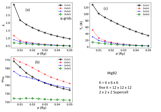


Convergence ansatz
Estimation of SC properties requires the computation of double-delta integration, which also defines the nesting function, around the Fermi level EF over the entire Brillouin zone [Eq. 3]. However, it has a slow convergence with respect to k- and q- grids. In principle, it requires infinitely dense grids, which makes the computation exorbitantly expensive. Therefore, Gaussian broadening technique [Eq. 5] is employed to compute with finite k-mesh. To compute Tc, we employed the DFPT calculation with the isotropic Eliashberg approximation. We used a coarse k-grid obtained from the MP database, which provides reasonably accurate ground-state properties. The q-grid was set to half the size of the k-grid, and a broadening parameter () of 0.01 Ry was utilized with the coarse MP grid, which accurately captures a converged electron-phonon coupling constant () of MgB2 computed using the anisotropic Migdal-Eliashberg equations [5]. However, in practice, is computed for a reasonable coarse k- and q- grids and interpolated the matrix elements to fine k- for any q-point, from 32 32 32 to as high as 60 60 60, to achieve numerical convergence, as implemented in Quantum Espresso (QE) code[3]. Furthermore, an efficient interpolation scheme utilizing both dense k- as well as q-grids has been implemented in EPW package that uses wannier orbitals [5]. However, employing extremely fine grids for interpolation can increase the computational complexity, which is not suitable for highthroughput calculations. Therefore, we have restricted ourselves for choosing fine k-grid only twice of corresponding coarse grid for highthroughput calculations.
Our investigation revealed that a reasonable number of calculations did not converge, leading to inaccurate predictions, while utilizing a coarse k-grid from MP database and fine grid for interpolation only twice that of the k-grid [Table ST3]. For example, AlB2 was predicted to be a superconductor (Tc 11 K) with the coarse grid [k-grid: 888, q-grid: 444, fine-k-mesh: 161616] from MP database, whereas a denser grid twice the size of the coarse grid corrected this inaccuracy and predicted AlB2 to be a nonsuperconductor, consistent with experimental observations [Fig. S7]. To identify such cases of convergence failure, we examined the variation of Tc with respect to and developed a simple ansatz based on the converged results of MgB2, as depicted in Fig. S9. The ansatz involves extracting Tc with a fixed broadening value (as in the case of MgB2) and estimating the decay parameter (A) in the exponential variation of Tc with as T. Unconverged results exhibit larger values of A, which decrease with a denser k-mesh.
The detail theory of EPC calculations within DFPT formalism in presented in the section “Theory of superconductivity: isotropic approximation”. The variation of density of states at the Fermi level () with respect to smearing , depends on Gaussian,
| (9) |
with also depends on . Despite of dependency of on EPC matrix () and phonon frequency () terms, the variation in is largely guided by the variation in or the Gaussian term G. Fig. S8(a)(a) shows the variation of G with respect to smearing for different values of , assuming independent of . The effect of on G dictates the variation of and hence Tc, with depends on the materials as well as on size of the grid to compute double delta integration. A larger represents more states contributing towards the double delta summation within space around the Fermi-level spanned by . In other word, will increase with if the density of states has local maximum close to the Fermi-level, and the variation of EPC properties will be similar to the Gaussian plots corresponding to 0.05. For Niobium, the variation of EPC properties with respect to follows similar to blue-dashed curve corresponding to = 0.01 [3], whereas for MgB2, the variation follows the Gaussian corresponding to 0.01. For and , if the Gaussian function recovers the delta function, while for the Gaussian drops to zero similar to 0.01 cases. Our primary focus is more on exponentially decaying cases.
The effect of smearing on is insignificant compared to or [2]. According to the BardeenCooperSchrieffer (BCS) theory [6],
| (10) |
where is the Debye cutoff energy and U is electron-phonon coupling potential. One can established the relation between or on as and with constant. Here parameter is a constant with a positive value if decreases with increasing and becomes negative otherwise. Here A and B are constants to be determined with A denoting the coefficient of exponential increase (for negative A) or decrease (for positive A) of with respect to . To determine the value of these constants, we perform linear-fit of vs for different k- grids for MgB2, which is frequently studied both theoretically as well as experimentally and often challenging to obtain the converged SC properties [7, 8, 9]. Furthermore, one can capture the behavior of Tc vs for a wide range of Tc using MgB2, as shown in Fig. S8(a)(b). We utilize a smaller k-mesh of 664 and a slightly larger k′-grid of 886 for comparison [Fig. S8(a)(b) and (c)].

Fig. S8(a) (b) represents the variation of with respect to , while Fig. S8(a) (c) presents vs plot. It exhibits nearly linear behavior up to , i.e. = 0.37, after which it deviates from linearity. The linear-fit has optimal coefficient of determination score (R2-score) for on vs data for k(charge density and EPC)-q(Phonon and EPC)-2k(interpolating EPC matrix) grids (Fig. S8(a) (c)) [Table within the Fig. S8(a)(c)]. Therefore, we chose in this work with R2-score of 0.9987. Besides different choice of leads to different values of A and B, it doesn’t have a significant role. For coarse grid, the Tc has a larger dependency on and shows larger exponential decay, compared to more converged calculations on denser grids. The exponential decay parameter “A” decreases from 19 to 10 with grids changing from coarse to dense one. This analysis suggests that A = 1213 can be used as a cutoff for this work, the calculations can be considered unconverged for A A, while the calculations can be considered converged for A A for accurate predictions. Fig. S8(a)(d) shows the convergence of the Tc with respect to q-point mesh, keeping k-grid fixed at 121212. A q-point grid as half as that of the ground-state k-point grid is sufficient to provide the converged results for MgB2. Fig. S8(a) (e) represents the spectral functions for various grids with k=886. Denser grid (2k) slightly blue shifts the spectral function peaks at lower frequency range (15.5-16.5 THz), while peaks at higher frequency ranges (20-22.5 THz) remain unaffected. This results slight change in from 0.78 to 0.72 and Tc changing from 20 K to 15-16 K [Figs. S1-S5]. A of 0.78 agrees with previous theoretical value of 0.75 from anisotropic Migdal-Eliashberg calculation using 0.16 [5], 0.71 from fully anisotropic SCDFT [10], and 0.73 from previous isotropic Eliashberg approximation [11] at slightly larger 0.015 Ry. This indicates a k-grid obtained from MP database with Ry already provide converged results in the case of MgB2. However, it is not always the case for other materials. Based on these results, parameters = 0.01 Ry with seems to be reasonable choice for smearing with 8 8 6 to 16 16 12 k-grids for MgB2, and for other systems for the sake of comparison. These parameters could also depend on pseudopotentials. In order to achieve converged results, it is necessary to use denser k- and q-grids. Subsequently, a double-delta integration should be performed, selecting the results that correspond to the limit of . Other details convergence tests of MgB2 with respect to Brillouin-zone sampling are presented in Figs. S2-S7.

In Fig. S8(b), we show two cases of YB12 and C2I2Y2 in which the coarse k- grids from Materials Project and fine k- grid only twice of that result to qualitatively inaccurate results, unusually high Tc for the former while predicting negligible Tc for the latter. With coarse grids, the exponential decay parameter of YB12 is around 38, much larger than the critical value estimated for MgB2 (A 12). Increasing k-mesh grids two times in each direction, Tc drops from 40.6 K to 1.67 K at 0.01 Ry and drops to almost zero for 0.01 Ry indicating non-superconductor, which is in good agreement with the experiment [12]. We found a couple of cases such as C2I2Y2 when first decreases and increases later with (we set A = 0 in Fig. S10). Such behavior hasn’t been observed in G(,) vs plots for a wide range of (Fig. 8(a) of the main text). The coarse grids result to a very low Tc of 0.97 K for C2I2Y2. However, the denser mesh corrects the behavior with an exponential decay parameter of 12.5 much closer to the reference value of MgB2. Also, the critical temperature Tc improves to 5.29 K agreeing much more strongly to the experiment [13]. Note that, this analysis only works for compounds with non-zero for a wide range of . For 1 K at Ry (computational details for choosing Ry), 0.1 K for Ry, and rapidly drops to zero for larger , we identify the compound to be non-superconducting with the value of A as zero (A = 0 A, already converged). To summarize the ansatz, we present a simple schematics of the process shown as in Fig. S9.

| Compound | (K) | (K) | (K) |
|---|---|---|---|
| YB12(Fm-3m) | 40.6 | 1.67 | 0 [12]222No transition observed above 2.5 K |
| CaNiBN (P4/nmm) | 0.96 | 2.43 | 2.2 [15] |
| BaC6 (P63/mmc) | 6.50 | 1.70 | 0 [16] |
| La3PbC (Pm-3m) | 3.20 | 0.50 | 0 [17]333No transition observed above 1 K |
| La3SnC (Pm-3m) | 5.09 | 0.81 | 0 [17] 444No transition observed above 1 K |
| CsC8 (P6/mmm) | 5.97 | 0.4 | 0.13 [20] |
| AlB2 (P6/mmm) | 11.3 | 0.3 | 0 [21] |
| C2I2Y2 (C2/m) | 0.97 | 5.29 | 9.97 [13] |
| C2Cl2Y2 (C2/m) | 0.508 | 2.73 | 2.3 [22] |
| Compound | (K) | (K) | (K) |
| WB (Cmcm) | 5.69 | 4.9 | 2.8 [23] |
| ReB2 (P63/mmc) | 0 | 0 | 0 [24] |
| LaB6 (Pm-3m) | 0.42 | 0 | 0.005 [25] |
| Ta2C (P-3m1) | 0.0 | 0.0 | 0 [26] |
| YIr3B2 (P6/mmm) | 5.5 | 5.54 | N/A 555Not reported |
| RuB2 (Pmmn) | 0.59 | 0.32 | 1.5 [28] |
| VC (Fm-3m) | 31.67 | 19.9 | 3.2 [29] |
| ZnNi3C (Pm-3m) | 15.37 | 15.4 | 0 [30]666No transition observed above 2.0 K |
| YRh3B2 (P6/mmm) | 5.8 | 4.2 | 0 [32] 777No transition observed above 1.5 K |
| YRu3B2 (P6/mmm) | 3.7 | 2.12 | 0 [34]888No transition observed above 1.2 K |
Next, we present results obtained from EPC calculations for 113 known boron and carbon superconducting (N = 53) and non-superconducting (N = 60) compounds from SuperCon database [36]. Fig. S10 represents the distribution of with respect to exponential decay parameter A for efficient calculations for Ry with . Based on the convergence check ansatz, we found that around 15 % (NoConv) of the results are not fully converged, while 70 % of them are qualitatively inaccurate (NoConv-False), compared to available experimental results. Similarly, we have 12 % of cases that have A A with qualitatively inaccurate predictions (Conv-False), which could be attributed from either inaccuracy of approximations to compute or inaccuracies within available experimental results. This work not only addresses the 15 % (NoConv) cases but also assists in validating true (Conv-True) results.

We present a few qualitatively inaccurate predictions with A A and improved results with a denser grid in Table ST3, while Table ST4 shows unaffected results (qualitatively) with denser grids for the cases with A A. For example, AlB2 is predicted to be superconductors with a coarse grid, while it changes to a non-superconductor with a denser grid, consistent with the experimental prediction. Similarly, of superconductors such as CaNiBN, C2I2Y2, and C2Cl2Y2 change from below 1 K (non-superconductor) to a larger value, and show a better agreement with the experiment. On the contrary, the qualitative results remain unchanged for converged calculations represented by A A, regardless of their agreement with the experimental references.
Application of convergence ansatz on known compounds of SuperCon
In this section, we compare the computed with available experimental results, as shown in Fig. S11 for efficient EPC calculations with and without improved data for A A (left panel) and A A (right panel) cases respectively. We also highlight some significantly deviated results with red rectangles for efficient calculations. With improved data, computed critical temperatures have much better agreement compared to the references, as indicated by the red rectangle enclosing more data points (right panel of Fig. S11), compared to the plot on the left. The results obtained from the ab-initio calculations demonstrate a notable level of accuracy with the mean absolute error (MAE) of 2.21 K for the critical temperature, compared to experiments, highlighting the reliability and robustness of this ansatz test. This is in comparison to the MAE of 3.18 K observed in efficient calculations. Please note that we have exclusively incorporated DFPT Tc results for systems that are dynamically stable. Despite the general agreement between DFPT and experimental findings, there exist notable discrepancies. Instances like ZnNi3C (Pm-3m), with a calculated Tc of 15 K, deviate enormously from the experimental values of 0 K [37]. A comparable investigation of ZnNi3C by Hoffmann et al.[38], utilizing different pseudopotentials from the PSEUDODOJO project[39], revealed phonon instabilities in these compounds. Notably, these unstable phonon modes were identified to possess significant mode-resolved EPC strength[40], a finding deserving attention, as we address these concerns in the “Imaginary Phonon Modes and Superconductivity” section. Similarly, Nb2InC (P63/mmc) with a calculated Tc of 0.34 K, VC (Fm-3m) at 20 K, and WB (I41/amd) at 18.5 K, present a problematic cases. Experimental Tc measurements stand at 3.2 K [29], 4.3 K [41], and 7.5 K [42] for VC, WB, and Nb2InC, respectively. These discrepancies can be ascribed to the constraints of both theoretical approaches and experimental procedures. For instance, older experimental investigations initially reported critical temperatures that were later rectified by more recent experiments or vice versa. For instance, in Ref [43], superconductivity below 4.7 K was claimed in certain YB12 samples, yet subsequent experiments, such as those in [44], failed to corroborate these findings. Furthermore, employing more sophisticated theoretical methodologies like solving the many-body anisotropic Migdal-Eliashberg equations or utilizing SCDFT to estimate Tc can significantly enhance the accuracy of calculations compared to isotropic methods. As an illustration, when examining MgB2, Tc calculated using isotropic Eliashberg theory falls within the 15-20 K range. However, in Ref. [45], Tc values of 34-42 K were reported over a range of values, demonstrating the improvement achievable with these advanced techniques.

In Table ST5, we show some of the inaccurate results predicting nonsuperconductors with 2D q- grids (441). Emergence of strong el-ph coupling and Tc with denser 3D q- grid (333) is unlikely for such nonsuperconducting predictions with Tc 0.01 K for 0.01 Ry [Fig. S9].
| Training size | CGCNN | ALIGNN | ||||||
|---|---|---|---|---|---|---|---|---|
| (k) | Tc (K) | T (K) | (K) | Tc (K) | T (K) | |||
| 250 (Run1) | 0.15 | 72 | 1.8 | 1.3 | 0.15 | 56 | 1.7 | 2.2 |
| 323 (Run2) | 0.27 | 85 | 6.4 | 5.5 | 0.16 | 83 | 3.0 | 3.3 |
| 351 (Run3) | 0.31 | 70 | 3.9 | 6.5 | 0.24 | 60 | 3.0 | 4.4 |
DFPT results for dynamically stable compounds
| ID | Compound | SG | FE (eV/atom) | (K) | Tc (K) | |
|---|---|---|---|---|---|---|
| mp-2252 | B2Sc1 | 191 | -0.84 | 0.34 | 606 | 0.032 |
| mp-10020 | C1Sc1 | 225 | -0.14 | 0.61 | 442 | 5.086 |
| mp-29941 | C1Sc2 | 164 | -0.42 | 0.24 | 351 | 0.0 |
| mp-1232372 | B2C2Sc2 | 194 | -0.6 | 0.21 | 565 | 0.0 |
| mp-27693 | B8C8Sc4 | 55 | -0.46 | 0.45 | 560 | 1.092 |
| mp-10343 | B1C2Sc2 | 139 | -0.57 | 0.41 | 467 | 0.383 |
| mp-10139 | B1Sc3Sn1 | 221 | -0.61 | 0.1 | 331 | 0.0 |
| mp-12062 | Ag1B2 | 191 | 0.52 | 0.88 | 568 | 21.563 |
| mp-7817 | B12Y1 | 225 | -0.24 | 0.48 | 605 | 1.69 |
| mp-1084 | B12Zr1 | 225 | -0.21 | 0.61 | 306 | 3.409 |
| mp-345 | B1Hf1 | 225 | -0.41 | 0.51 | 281 | 1.225 |
| mp-1890 | B4Mo4 | 141 | -0.5 | 0.4 | 364 | 0.228 |
| mp-999198 | B2Mo2 | 63 | -0.49 | 0.63 | 338 | 4.398 |
| mp-451 | B1Zr1 | 225 | -0.37 | 0.47 | 383 | 0.946 |
| mp-763 | B2Mg1 | 191 | -0.13 | 0.78 | 734 | 20.027 |
| mp-450 | B2Nb1 | 191 | -0.69 | 0.72 | 365 | 7.68 |
| mp-1773 | B4Re2 | 194 | -0.43 | 0.22 | 409 | 0.0 |
| mp-1077 | B4Ru2 | 59 | -0.29 | 0.42 | 364 | 0.356 |
| mp-1472 | B2Zr1 | 191 | -0.99 | 0.14 | 581 | 0.0 |
| mp-2680 | B6La1 | 221 | -0.56 | 0.26 | 343 | 0.0 |
| mp-2203 | B6Y1 | 221 | -0.4 | 1.97 | 81 | 9.999 |
| mp-1079500 | B2Ca2N2Ni2 | 129 | -0.97 | 0.53 | 464 | 2.474 |
| mp-1106180 | B6Re14 | 186 | -0.22 | 0.72 | 180 | 3.83 |
| mp-15671 | B2Re6 | 63 | -0.2 | 0.72 | 209 | 4.4 |
| mp-2850 | B4Os2 | 59 | -0.21 | 0.61 | 263 | 3.07 |
| mp-21502 | B4Rh8 | 62 | -0.21 | 0.65 | 183 | 2.692 |
| mp-7857 | B4Ti4 | 62 | -0.83 | 0.27 | 443 | 0.0 |
| mp-20881 | B2La2N2Ni2 | 129 | -1.05 | 0.64 | 301 | 4.241 |
| mp-9219 | B2C1La1Pt2 | 139 | -0.64 | 0.76 | 262 | 6.732 |
| mp-3465 | B2La1Rh3 | 191 | -0.67 | 0.84 | 174 | 5.859 |
| mp-6114 | B2La3N3Ni2 | 139 | -1.15 | 0.61 | 362 | 4.056 |
| mp-20234 | B4Li8Pt12 | 212 | -0.57 | 1.31 | 96 | 7.615 |
| mp-4984 | B4Mo10Si2 | 140 | -0.4 | 0.81 | 257 | 7.838 |
| mp-1189073 | B8Os4Sc4 | 62 | -0.68 | 0.63 | 330 | 4.305 |
| mp-1105309 | B4Ge2Ta10 | 140 | -0.59 | 0.29 | 234 | 0.0 |
| mp-1078866 | B4C4Y2 | 127 | -0.44 | 0.52 | 455 | 2.323 |
| mp-15955 | B4C4Y2 | 131 | -0.3 | 0.5 | 392 | 1.531 |
| mp-1024989 | B2C1Pd2Y1 | 139 | -0.5 | 1.14 | 249 | 15.971 |
| mp-5984 | B8Rh8Y2 | 137 | -0.59 | 0.77 | 223 | 5.866 |
| mp-1190832 | B16Ru4Y4 | 55 | -0.62 | 0.28 | 501 | 0.0 |
| mp-980205 | B16Os4Y4 | 55 | -0.57 | 0.28 | 404 | 0.0 |
| mp-2091 | B4V6 | 127 | -0.72 | 0.23 | 473 | 0.0 |
| mp-260 | B2Cr2 | 63 | -0.52 | 0.45 | 412 | 0.68 |
| mp-9973 | B2V2 | 63 | -0.85 | 0.23 | 508 | 0.0 |
| mp-1183252 | B1Ir1 | 187 | -0.2 | 0.47 | 214 | 0.539 |
| mp-567164 | B2Rh2 | 194 | -0.39 | 0.15 | 313 | 0.0 |
| mp-1063752 | B2Rh2 | 194 | -0.18 | 0.91 | 173 | 7.127 |
| mp-4472 | B2C2Mo4 | 63 | -0.25 | 0.78 | 199 | 5.414 |
| mp-10112 | B2Ir3La1 | 191 | -0.65 | 0.62 | 151 | 1.828 |
| mp-2536 | B2Ni4 | 140 | -0.29 | 0.22 | 316 | 0.0 |
| mp-1080664 | B4Cr4 | 141 | -0.53 | 0.27 | 449 | 0.0 |
| mp-1994 | B2Hf1 | 191 | -1.02 | 0.16 | 518 | 0.0 |
| mp-2331 | B4Mo2 | 166 | -0.43 | 0.4 | 437 | 0.239 |
| mp-20689 | B4Nb6 | 127 | -0.63 | 0.26 | 365 | 0.0 |
| mp-13415 | B4Ta6 | 127 | -0.67 | 0.24 | 306 | 0.0 |
| ID | Compound | SG | FE (eV/atom) | (K) | Tc (K) | |
|---|---|---|---|---|---|---|
| mp-1491 | B2V1 | 191 | -0.74 | 0.29 | 494 | 0.001 |
| mp-8431 | B4Ca2Rh4 | 70 | -0.61 | 0.26 | 325 | 0.0 |
| mp-1008487 | B2W2 | 63 | -0.36 | 0.68 | 274 | 4.902 |
| mp-10142 | B4Ta3 | 71 | -0.77 | 0.36 | 357 | 0.046 |
| mp-865 | Ca1B6 | 221 | -0.41 | 0.16 | 538 | 0.0 |
| mp-14445 | B4Ca2Ir4 | 70 | -0.68 | 0.26 | 338 | 0.0 |
| mp-944 | Al1B2 | 191 | -0.04 | 0.4 | 564 | 0.295 |
| mp-10852 | B4C4La2 | 127 | -0.44 | 0.38 | 420 | 0.113 |
| mp-7783 | B4C4La2 | 131 | -0.31 | 0.5 | 459 | 1.862 |
| mp-2967 | B2Co2La1 | 139 | -0.48 | 0.31 | 304 | 0.002 |
| mp-5992 | B2C1Ir2La1 | 139 | -0.57 | 0.36 | 250 | 0.035 |
| mp-568083 | B2C1La1Ni2 | 139 | -0.44 | 0.33 | 299 | 0.009 |
| mp-6794 | B2C1La1Rh2 | 139 | -0.6 | 0.35 | 284 | 0.022 |
| mp-571428 | B6Mg3Ni9 | 181 | -0.38 | 0.2 | 353 | 0.0 |
| mp-4938 | B2Co3Sc1 | 191 | -0.55 | 0.37 | 275 | 0.07 |
| mp-6939 | B4Ir4Sr2 | 70 | -0.63 | 0.28 | 351 | 0.0 |
| mp-7348 | B4Rh4Sr2 | 70 | -0.56 | 0.23 | 335 | 0.0 |
| mp-3515 | B2Co2Y1 | 139 | -0.56 | 0.24 | 383 | 0.0 |
| mp-1024941 | B2Rh3Y1 | 191 | -0.71 | 0.76 | 162 | 4.181 |
| mp-4382 | B2Ru3Y1 | 191 | -0.47 | 0.62 | 172 | 2.121 |
| mp-9956 | Al2C2Cr4 | 194 | -0.17 | 0.24 | 403 | 0.0 |
| mp-3271 | Al1C1Ti3 | 221 | -0.59 | 0.28 | 271 | 0.0 |
| mp-1025497 | Al2C2V4 | 194 | -0.52 | 0.23 | 425 | 0.0 |
| mp-4448 | Y3Al1C1 | 221 | -0.42 | 0.1 | 254 | 0.0 |
| mp-1190604 | Al8C4Nb12 | 213 | -0.46 | 0.35 | 256 | 0.022 |
| mp-1190760 | Al8C4Ta12 | 213 | -0.45 | 0.4 | 191 | 0.111 |
| mp-1214417 | Ba2C12 | 194 | -0.09 | 0.53 | 300 | 1.709 |
| mp-9961 | C2Cd2Ti4 | 194 | -0.54 | 0.28 | 233 | 0.0 |
| mp-21075 | C1Hf1 | 225 | -0.94 | 0.13 | 457 | 0.0 |
| mp-1096993 | C2Hf2 | 194 | -0.74 | 0.46 | 416 | 0.865 |
| mp-1002124 | Hf1C1 | 216 | -0.3 | 0.05 | 424 | 0.023 |
| mp-10611 | C1La3Pb1 | 221 | -0.43 | 0.49 | 151 | 0.516 |
| mp-1206443 | C1La3Sn1 | 221 | -0.49 | 0.53 | 146 | 0.806 |
| mp-5443 | C2Nb4Sn2 | 194 | -0.42 | 0.45 | 271 | 0.527 |
| mp-20661 | C2Pb2Ti4 | 194 | -0.57 | 0.31 | 321 | 0.004 |
| mp-631 | C1Ti1 | 225 | -0.81 | 0.16 | 601 | 0.0 |
| mp-1282 | C1V1 | 225 | -0.41 | 1.14 | 312 | 19.989 |
| mp-20648 | C4V8 | 60 | -0.47 | 0.3 | 348 | 0.001 |
| mp-1008632 | C1V2 | 164 | -0.45 | 0.24 | 319 | 0.0 |
| mp-2795 | C1Zr1 | 225 | -0.8 | 0.15 | 484 | 0.0 |
| mp-1014307 | C2Zr2 | 194 | -0.64 | 0.41 | 480 | 0.321 |
| mp-570112 | C4Cr6 | 63 | -0.07 | 0.55 | 343 | 2.407 |
| mp-28861 | C8Cs1 | 191 | -0.05 | 0.4 | 766 | 0.438 |
| mp-568643 | C16Rb2 | 70 | -0.04 | 0.5 | 755 | 2.902 |
| mp-16290 | C1Ni3Zn1 | 221 | -0.06 | 1.94 | 126 | 15.406 |
| mp-1066566 | C2Ni1Y1 | 38 | -0.33 | 0.47 | 395 | 1.074 |
| mp-1079635 | C2Ga2Mo4 | 194 | -0.12 | 0.77 | 249 | 6.627 |
| mp-2305 | C1Mo1 | 187 | -0.08 | 0.18 | 512 | 0.0 |
| mp-1552 | C4Mo8 | 60 | -0.11 | 0.7 | 272 | 5.298 |
| mp-1221498 | C1Mo2 | 164 | -0.05 | 0.6 | 287 | 3.119 |
| mp-910 | C1Nb1 | 225 | -0.46 | 1.11 | 309 | 18.924 |
| mp-1094093 | C2Nb2 | 194 | -0.35 | 1.14 | 300 | 19.284 |
| mp-999388 | C2Nb2 | 194 | -0.33 | 0.84 | 455 | 15.269 |
| mp-999377 | C2Nb2 | 194 | -0.09 | 0.71 | 320 | 6.7 |
| mp-1086 | C1Ta1 | 225 | -0.58 | 0.68 | 236 | 4.239 |
| ID | Compound | SG | FE (eV/atom) | (K) | Tc (K) | |
|---|---|---|---|---|---|---|
| mp-1009832 | C1Ta1 | 216 | -0.06 | 0.69 | 213 | 4.034 |
| mp-7088 | C1Ta2 | 164 | -0.6 | 0.22 | 250 | 0.0 |
| mp-2034 | C4W8 | 60 | -0.02 | 0.77 | 212 | 5.512 |
| mp-33065 | C2W4 | 58 | -0.01 | 0.79 | 213 | 6.119 |
| mp-2367 | C2La1 | 139 | -0.16 | 0.5 | 258 | 0.978 |
| mp-313 | C2Y1 | 139 | -0.19 | 0.83 | 282 | 9.383 |
| mp-1208630 | C12Sr2 | 194 | -0.04 | 0.67 | 310 | 5.291 |
| mp-1018048 | C2La1Ni1 | 38 | -0.25 | 0.71 | 346 | 6.943 |
| mp-1206284 | Br2C2La2 | 12 | -1.12 | 0.7 | 174 | 3.416 |
| mp-20315 | C2In2Ti4 | 194 | -0.67 | 0.13 | 352 | 0.0 |
| mp-643367 | Br2C2Y2 | 12 | -1.08 | 0.77 | 251 | 6.614 |
| mp-37919 | Br2C2Y2 | 59 | -0.08 | 1.21 | 109 | 7.789 |
| mp-23062 | C2I2Y2 | 12 | -0.86 | 0.77 | 196 | 5.177 |
| mp-1206889 | C2Cl2Y2 | 12 | -1.44 | 0.6 | 258 | 2.725 |
| mp-6576 | B2C1Ni2Y1 | 139 | -0.51 | 0.59 | 315 | 3.159 |
| mp-2192 | B2Pt2 | 194 | 0.07 | 1.24 | 188 | 13.786 |
| mp-1009218 | C1Mo1 | 216 | 0.5 | 1.71 | 103 | 11.153 |
| mp-632442 | Al4C3 | 1 | 0.31 | 0.6 | 256 | 2.704 |
| mp-1076 | KB6 | 221 | -0.03 | 0.51 | 823 | 3.715 |
| mp-1078278 | CrB4 | 58 | -0.31 | 0.25 | 622 | 0.0 |
| mp-1079437 | FeB4 | 58 | -0.17 | 0.9 | 468 | 18.723 |
| mp-1080111 | B3Mo | 166 | -0.31 | 0.29 | 574 | 0.001 |
| mp-1106184 | MnB4 | 14 | -0.29 | 0.14 | 559 | 0.0 |
| mp-1213975 | CaB4 | 127 | -0.39 | 0.25 | 551 | 0.0 |
| mp-1228730 | B24Mo7 | 187 | -0.14 | 1.33 | 359 | 28.901 |
| mp-2315 | NaB15 | 74 | -0.05 | 0.1 | 763 | 0.0 |
| mp-262 | Na3B20 | 65 | -0.06 | 0.4 | 782 | 0.513 |
| mp-27710 | CrB4 | 71 | -0.3 | 0.23 | 755 | 0.0 |
| mp-576 | B13C2 | 166 | -0.07 | 0.97 | 835 | 39.304 |
| mp-637 | YB4 | 127 | -0.59 | 0.43 | 388 | 0.457 |
| mp-7283 | LaB4 | 127 | -0.56 | 0.28 | 465 | 0.0 |
| mp-1218188 | SrLaB12 | 123 | -0.51 | 0.36 | 306 | 0.041 |
| mp-1232339 | LiC12 | 63 | -0.0 | 0.43 | 1055 | 1.24 |
| mp-1227841 | BaLaB12 | 123 | -0.49 | 0.36 | 304 | 0.052 |
| mp-1001581 | LiC6 | 191 | -0.0 | 0.39 | 1043 | 0.397 |
| mp-1021323 | LiC12 | 191 | -0.01 | 0.33 | 949 | 0.035 |
| mp-1001835 | LiB | 194 | -0.17 | 0.21 | 328 | 0.0 |
| mp-1002188 | TcB | 187 | -0.28 | 0.4 | 445 | 0.267 |
| mp-1009695 | CaB2 | 191 | -0.14 | 0.68 | 444 | 7.604 |
| mp-1224328 | HfNbB4 | 191 | -0.86 | 0.33 | 462 | 0.013 |
| mp-1019317 | TcB2 | 194 | -0.44 | 0.27 | 497 | 0.0 |
| mp-1025170 | Ti3B4 | 71 | -0.93 | 0.25 | 517 | 0.0 |
| mp-1217974 | TaB4W3 | 25 | -0.48 | 0.6 | 277 | 2.921 |
| mp-1080021 | Nb2B3 | 63 | -0.75 | 0.45 | 409 | 0.777 |
| mp-1217965 | TaB2Mo | 38 | -0.66 | 0.57 | 348 | 2.788 |
| mp-1102394 | Nb5B6 | 65 | -0.77 | 0.4 | 398 | 0.209 |
| mp-1108 | TaB2 | 191 | -0.65 | 1.22 | 253 | 18.116 |
| mp-1217924 | TaNbC2 | 166 | -0.52 | 1.41 | 326 | 28.387 |
| mp-1217818 | TaVB4 | 191 | -0.69 | 0.6 | 387 | 4.047 |
| mp-1206441 | V5B6 | 65 | -0.83 | 0.26 | 488 | 0.0 |
| mp-1207750 | Y5(SiB4)2 | 127 | -0.68 | 0.33 | 401 | 0.014 |
| mp-1217023 | TiB2W | 38 | -0.78 | 0.3 | 419 | 0.001 |
| mp-1079333 | B2CN | 51 | -0.53 | 0.46 | 1045 | 2.381 |
| mp-13854 | B3Ru2 | 194 | -0.33 | 0.14 | 445 | 0.0 |
| mp-14019 | NiB | 63 | -0.24 | 0.24 | 376 | 0.0 |
| ID | Compound | SG | FE (eV/atom) | (K) | Tc (K) | |
|---|---|---|---|---|---|---|
| mp-1216709 | TiNbB2 | 38 | -0.81 | 0.31 | 472 | 0.005 |
| mp-20857 | CoB | 62 | -0.4 | 0.11 | 357 | 0.0 |
| mp-2580 | NbB | 63 | -0.77 | 0.31 | 415 | 0.005 |
| mp-1215250 | ZrB4Mo | 191 | -0.62 | 1.3 | 193 | 15.047 |
| mp-569803 | B2W | 194 | -0.33 | 0.48 | 323 | 0.999 |
| mp-999120 | TcB | 194 | -0.22 | 0.42 | 378 | 0.335 |
| mp-1215178 | ZrTiB4 | 191 | -1.0 | 0.09 | 617 | 0.0 |
| mp-9208 | V2B3 | 63 | -0.8 | 0.29 | 488 | 0.001 |
| mp-999118 | TcB | 194 | -0.12 | 1.32 | 332 | 26.488 |
| mp-12054 | Cr2B3 | 63 | -0.43 | 0.56 | 358 | 2.753 |
| mp-10114 | ScB4Ir3 | 176 | -0.59 | 0.18 | 258 | 0.0 |
| mp-9880 | YB2C | 135 | -0.52 | 0.32 | 506 | 0.012 |
| mp-995282 | LiAlB4 | 55 | -0.05 | 0.5 | 693 | 2.659 |
| mp-1008527 | B2CN | 115 | -0.44 | 0.8 | 644 | 18.759 |
| mp-1207086 | MgAlB4 | 191 | -0.15 | 0.34 | 769 | 0.059 |
| mp-1215209 | ZrTaB4 | 191 | -0.84 | 0.39 | 436 | 0.177 |
| mp-1215223 | ZrNbB2 | 38 | -0.71 | 0.35 | 404 | 0.04 |
| mp-1216966 | TiCrB4 | 191 | -0.68 | 0.59 | 339 | 3.385 |
| mp-1217028 | TiB2Mo | 38 | -0.82 | 0.25 | 461 | 0.0 |
| mp-1220697 | Nb2AlB6 | 191 | -0.47 | 0.54 | 431 | 2.781 |
| mp-1224283 | HfTaB4 | 191 | -0.85 | 0.41 | 423 | 0.354 |
| mp-1224291 | HfTaB2 | 38 | -0.77 | 0.4 | 354 | 0.199 |
| mp-1224347 | HfNbB2 | 38 | -0.76 | 0.37 | 387 | 0.073 |
| mp-1226228 | CrB2Mo | 38 | -0.48 | 0.62 | 331 | 3.919 |
| mp-13341 | YB4Rh | 55 | -0.61 | 0.62 | 483 | 6.008 |
| mp-568985 | La2B3Br | 187 | -0.84 | 0.35 | 212 | 0.018 |
| mp-569002 | Y3ReB7 | 63 | -0.33 | 0.81 | 330 | 9.953 |
| mp-1008526 | B2CN | 156 | -0.42 | 1.11 | 566 | 34.9 |
| mp-569121 | La2B3Cl | 174 | -1.02 | 0.41 | 209 | 0.158 |
| mp-1191641 | YVB4 | 55 | -0.7 | 0.3 | 473 | 0.001 |
| mp-1216398 | VCrB2 | 38 | -0.69 | 0.39 | 460 | 0.19 |
| mp-1216475 | V3ReB4 | 25 | -0.72 | 0.39 | 391 | 0.169 |
| mp-1216667 | TiVB4 | 191 | -0.9 | 0.27 | 516 | 0.0 |
| mp-1217026 | TiB4Mo | 191 | -0.68 | 0.69 | 348 | 6.374 |
| mp-1217095 | Ti3B4Mo | 6 | -0.83 | 0.28 | 454 | 0.0 |
| mp-1217898 | TaTiB4 | 191 | -0.88 | 0.29 | 441 | 0.001 |
| mp-1217997 | Ta3AlB8 | 191 | -0.5 | 0.54 | 316 | 1.858 |
| mp-1220349 | NbB2W | 38 | -0.58 | 0.57 | 341 | 2.717 |
| mp-1220351 | NbVB4 | 191 | -0.71 | 0.51 | 421 | 1.948 |
| mp-1220383 | NbB4Mo3 | 38 | -0.56 | 0.58 | 354 | 3.101 |
| mp-1008525 | B2CN | 160 | -0.43 | 1.66 | 577 | 60.733 |
| mp-10057 | VCoB3 | 63 | -0.62 | 0.26 | 438 | 0.0 |
| mp-1226242 | CrB2W | 38 | -0.43 | 0.74 | 290 | 6.877 |
| mp-1228634 | B4MoIr | 187 | -0.25 | 0.5 | 280 | 1.054 |
| mp-1196778 | Y2B6Ru | 55 | -0.66 | 0.22 | 511 | 0.0 |
| mp-22709 | TaNiB2 | 62 | -0.63 | 0.3 | 324 | 0.001 |
| mp-569116 | Sc2B6Rh | 55 | -0.73 | 0.52 | 414 | 2.079 |
| mp-1224274 | HfTiC2 | 166 | -0.83 | 0.42 | 464 | 0.462 |
| mp-1215222 | ZrNbC2 | 166 | -0.66 | 0.73 | 397 | 8.92 |
| mp-1224334 | HfNbC2 | 166 | -0.73 | 0.65 | 385 | 5.753 |
| mp-1018050 | CrC | 187 | -0.0 | 0.23 | 610 | 0.0 |
| mp-1215480 | Zr3NbC4 | 166 | -0.73 | 0.77 | 346 | 9.324 |
| mp-1216691 | TiVC2 | 166 | -0.62 | 0.53 | 446 | 2.47 |
| mp-1215174 | ZrTiC2 | 123 | -0.71 | 0.25 | 461 | 0.0 |
| mp-1215218 | ZrMoC2 | 166 | -0.35 | 1.79 | 120 | 13.656 |
| ID | Compound | SG | FE (eV/atom) | (K) | Tc (K) | |
|---|---|---|---|---|---|---|
| mp-38818 | HfNbB4 | 71 | -0.86 | 0.4 | 420 | 0.254 |
| mp-1086667 | ScNiC2 | 129 | -0.28 | 0.52 | 368 | 1.864 |
| mp-1217975 | Ta3TiB4 | 25 | -0.84 | 0.26 | 394 | 0.0 |
| mp-9530 | Y4C7 | 14 | -0.28 | 0.13 | 323 | 0.0 |
| mp-9459 | Y4C5 | 55 | -0.33 | 0.84 | 225 | 7.678 |
| mp-1188534 | ScCrC2 | 59 | -0.34 | 0.62 | 389 | 4.881 |
| mp-1224170 | HfZrC2 | 123 | -0.87 | 0.25 | 483 | 0.0 |
| mp-1334 | Y2C | 166 | -0.29 | 0.29 | 201 | 0.0 |
| mp-1232379 | YBC | 194 | -0.29 | 0.28 | 427 | 0.0 |
| mp-29896 | Y2B3C2 | 65 | -0.5 | 0.6 | 375 | 3.915 |
| mp-612670 | YNiBC | 129 | -0.52 | 0.2 | 421 | 0.0 |
| mp-567692 | B4C3Ni4Y3 | 139 | -0.51 | 0.31 | 393 | 0.003 |
| mp-12737 | B2C1Rh2Y1 | 139 | -0.6 | 0.38 | 285 | 0.098 |
| mp-1087495 | Tc3B | 63 | -0.27 | 0.8 | 254 | 7.66 |
| mp-978989 | Tc7B3 | 186 | -0.32 | 0.68 | 227 | 4.037 |
| mp-1068296 | Fe(BW)2 | 71 | -0.43 | 0.45 | 279 | 0.465 |
| mp-11750 | Ti6Si2B | 189 | -0.66 | 0.22 | 333 | 0.0 |
| mp-1238800 | CaBC | 194 | -0.07 | 0.42 | 501 | 0.494 |
| mp-27261 | Ba7(BIr)12 | 166 | -0.48 | 0.47 | 233 | 0.626 |
| mp-29980 | Nb4B3C2 | 63 | -0.59 | 1.01 | 219 | 11.258 |
| mp-29979 | Nb3B3C | 63 | -0.66 | 1.22 | 229 | 16.438 |
| mp-541849 | Al3(BRu2)2 | 123 | -0.59 | 0.26 | 308 | 0.0 |
| mp-1188408 | Zr5Sn3B | 193 | -0.68 | 0.45 | 202 | 0.343 |
| mp-1206909 | CaBPd3 | 221 | -0.56 | 1.1 | 103 | 6.187 |
| mp-9985 | NbNiB | 63 | -0.56 | 0.34 | 256 | 0.018 |
| mp-1080829 | Ti6Ge2B | 189 | -0.62 | 0.21 | 305 | 0.0 |
| mp-1025192 | Ta4C3 | 221 | -0.45 | 1.46 | 138 | 12.644 |
| mp-1215211 | ZrNbB4 | 191 | -0.85 | 0.31 | 479 | 0.005 |
| mp-1220641 | Nb3B4W3 | 38 | -0.43 | 0.46 | 299 | 0.66 |
| mp-10721 | Ti2C | 227 | -0.64 | 0.14 | 386 | 0.0 |
| mp-27919 | Ti8C5 | 166 | -0.72 | 0.22 | 455 | 0.0 |
| mp-1218000 | Ta4C3 | 160 | -0.55 | 0.52 | 183 | 0.919 |
| mp-1220752 | Nb10(SiB)3 | 42 | -0.65 | 0.24 | 310 | 0.0 |
| mp-1189539 | Hf2Al3C5 | 194 | -0.13 | 0.47 | 1454 | 3.645 |
| mp-9958 | Ti2GeC | 194 | -0.81 | 0.48 | 276 | 0.847 |
| mp-1025524 | Zr2TlC | 194 | -0.63 | 0.21 | 188 | 0.0 |
| mp-1216707 | TiNbC2 | 166 | -0.67 | 0.73 | 422 | 9.623 |
| mp-1079992 | Zr2PbC | 194 | -0.66 | 0.4 | 230 | 0.146 |
| mp-1207413 | Zr5Sn3C | 193 | -0.68 | 0.53 | 180 | 1.013 |
| mp-1217106 | Ti2C | 166 | -0.63 | 0.35 | 357 | 0.037 |
| mp-1217822 | TaVC2 | 166 | -0.46 | 0.8 | 343 | 10.296 |
| mp-12990 | Ti2AlC | 194 | -0.7 | 0.25 | 371 | 0.0 |
| mp-3871 | Ti2SnC | 194 | -0.73 | 0.24 | 353 | 0.0 |
| mp-1025427 | Ta2GaC | 194 | -0.52 | 0.45 | 231 | 0.385 |
| mp-1078712 | Hf2TlC | 194 | -0.63 | 0.21 | 171 | 0.0 |
| mp-1079076 | Hf2PbC | 194 | -0.63 | 0.41 | 194 | 0.15 |
| mp-1079908 | Ti2SiC | 194 | -0.79 | 0.4 | 334 | 0.205 |
| mp-1220365 | NbVC2 | 166 | -0.39 | 0.83 | 365 | 11.893 |
| mp-21023 | Ti3SnC2 | 194 | -0.79 | 0.18 | 421 | 0.0 |
| mp-22144 | Ta2InC | 194 | -0.38 | 0.37 | 233 | 0.062 |
| mp-4893 | Hf2SnC | 194 | -0.78 | 0.31 | 205 | 0.003 |
| mp-5659 | Ti3SiC2 | 194 | -0.82 | 0.37 | 345 | 0.081 |
| mp-1092281 | Ti2TlC | 194 | -0.57 | 0.14 | 295 | 0.0 |
| mp-3747 | Ti3AlC2 | 194 | -0.76 | 0.26 | 342 | 0.0 |
| mp-3886 | Zr2AlC | 194 | -0.64 | 0.56 | 163 | 1.181 |
| ID | Compound | SG | FE (eV/atom) | (K) | Tc (K) | |
|---|---|---|---|---|---|---|
| mp-13137 | Hf2CS | 194 | -1.51 | 0.19 | 303 | 0.0 |
| mp-1220725 | Nb2CN | 166 | -0.8 | 0.88 | 310 | 11.685 |
| mp-1216616 | V2CN | 166 | -0.8 | 1.0 | 322 | 16.224 |
| mp-1214755 | BPd6 | 15 | -0.2 | 0.16 | 169 | 0.0 |
| mp-7424 | BPd2 | 58 | -0.27 | 0.42 | 159 | 0.16 |
| mp-1078540 | Ni6Ge2B | 189 | -0.31 | 0.34 | 190 | 0.011 |
| mp-1078623 | Zr2BIr6 | 225 | -0.81 | 0.36 | 184 | 0.03 |
| mp-12073 | Ba(BIr)2 | 139 | -0.5 | 0.37 | 269 | 0.051 |
| mp-7349 | Ba(BRh)2 | 139 | -0.48 | 0.29 | 295 | 0.001 |
| mp-7705 | NbFeB | 187 | -0.12 | 1.76 | 162 | 18.063 |
| mp-1215258 | ZrBeB | 187 | -0.58 | 0.45 | 436 | 0.751 |
| mp-1208348 | Ta5Ga3B | 193 | -0.42 | 0.31 | 190 | 0.002 |
| mp-605839 | Li2B2Rh3 | 55 | -0.5 | 0.27 | 302 | 0.0 |
| mp-8308 | Ca3Ni7B2 | 166 | -0.34 | 0.13 | 305 | 0.0 |
| mp-1206490 | Nb2B2Mo | 127 | -0.64 | 0.28 | 367 | 0.0 |
| mp-31052 | LaBPt2 | 180 | -0.92 | 0.28 | 142 | 0.0 |
| mp-1223681 | La2(Ni2B)3 | 44 | -0.33 | 0.46 | 227 | 0.517 |
| mp-1097 | B2Ta2 | 63 | -0.81 | 0.41 | 366 | 0.297 |
| mp-28930 | C16K2 | 70 | -0.03 | 0.57 | 1102 | 8.897 |
| mp-7832 | B4W4 | 141 | -0.37 | 0.45 | 301 | 0.523 |
| mp-28613 | B3Li3Pt9 | 189 | -0.51 | 0.4 | 152 | 0.101 |
| mp-569759 | B4Rh8Zn5 | 65 | -0.42 | 0.26 | 223 | 0.0 |
| mp-571419 | Al4C5Zr2 | 166 | -0.35 | 0.36 | 384 | 0.06 |
| mp-1207385 | Al8C8Zr2 | 164 | -0.25 | 0.26 | 481 | 0.0 |
| mp-1189895 | B2Ge6Ta10 | 193 | -0.45 | 0.61 | 180 | 2.075 |
| mp-10140 | B1Sc3Tl1 | 221 | -0.36 | 0.53 | 219 | 1.247 |
| mp-1216165 | B1Si6Y10 | 162 | -0.65 | 0.4 | 169 | 0.092 |
| mp-20175 | C2In2Sc4 | 194 | -0.55 | 0.21 | 171 | 0.0 |
| mp-20983 | C2In2V4 | 194 | -0.34 | 0.35 | 349 | 0.03 |
| mp-1224263 | B4Hf1Ti1 | 191 | -1.02 | 0.1 | 592 | 0.0 |
| mp-1224184 | B4Hf1Zr1 | 47 | -1.0 | 0.15 | 507 | 0.0 |
| mp-8307 | B2Ca2Ni8 | 191 | -0.3 | 0.33 | 131 | 0.004 |
| mp-4079 | Al1C1Sc3 | 221 | -0.59 | 0.04 | 299 | 0.047 |
| mp-1103814 | C3K5N6 | 229 | -0.52 | 0.08 | 199 | 0.0 |
| mp-1224285 | C2Hf1Ta1 | 166 | -0.81 | 0.64 | 346 | 4.709 |
| mp-1215219 | C2Ta1Zr1 | 166 | -0.74 | 0.65 | 370 | 5.558 |
| mp-570499 | B2La5N6 | 12 | -1.51 | 0.25 | 350 | 0.0 |
| mp-569935 | B2La3N4 | 71 | -1.5 | 0.26 | 378 | 0.0 |
| mp-1223086 | C6La2Y1 | 12 | -0.16 | 0.56 | 271 | 2.049 |
| mp-1221519 | C1Mo2N1 | 25 | -0.35 | 0.37 | 472 | 0.105 |
| mp-1222150 | Al1B10Mg4 | 191 | -0.14 | 0.59 | 768 | 7.488 |
| mp-1189984 | C8Mo4Y4 | 62 | -0.24 | 0.61 | 409 | 4.562 |
| mp-3380 | C8La4Rh4 | 76 | -0.33 | 0.27 | 259 | 0.0 |
| mp-4262 | BeAlB | 216 | -0.05 | 0.16 | 578 | 0.0 |
| mp-5971 | YBPt2 | 180 | -1.0 | 0.18 | 191 | 0.0 |
| mp-9596 | La(BIr)4 | 86 | -0.58 | 0.47 | 201 | 0.503 |
| mp-1105186 | Cu3B5Pt9 | 189 | -0.21 | 0.4 | 164 | 0.099 |
| mp-1106165 | Nb5Si3B | 193 | -0.69 | 0.46 | 282 | 0.638 |
| mp-1106398 | V5Ge3B | 193 | -0.46 | 0.38 | 303 | 0.11 |
| mp-1188194 | Ta3B2Ru5 | 127 | -0.53 | 0.33 | 146 | 0.006 |
| mp-1188856 | V5Si2B | 140 | -0.39 | 0.37 | 302 | 0.067 |
| mp-1216445 | V9Cr3B8 | 10 | -0.7 | 0.25 | 459 | 0.0 |
| mp-1216643 | V10Si6B | 162 | -0.63 | 0.33 | 323 | 0.014 |
| mp-1220688 | Nb3Re3B4 | 38 | -0.35 | 0.53 | 265 | 1.47 |
| mp-1226327 | Cr3B4Mo3 | 38 | -0.29 | 0.78 | 289 | 8.091 |
| ID | Compound | SG | FE (eV/atom) | (K) | Tc (K) | |
|---|---|---|---|---|---|---|
| mp-29723 | LaB2Ru3 | 191 | -0.41 | 0.67 | 148 | 2.477 |
| mp-22759 | CoBW | 62 | -0.43 | 0.37 | 342 | 0.071 |
| mp-28786 | Zn(BIr)2 | 139 | -0.32 | 0.08 | 319 | 0.0 |
| mp-9999 | Ni(BMo)2 | 71 | -0.48 | 0.3 | 352 | 0.001 |
| mp-1076987 | TaNiB | 63 | -0.62 | 0.3 | 253 | 0.001 |
| mp-3348 | LiBIr | 70 | -0.51 | 0.16 | 325 | 0.0 |
| mp-2760 | Nb6C5 | 12 | -0.55 | 0.51 | 393 | 1.632 |
| mp-32679 | Nb10C7 | 12 | -0.48 | 0.45 | 301 | 0.537 |
| mp-1226378 | Cr2C | 164 | -0.04 | 0.38 | 376 | 0.118 |
| mp-2318 | Nb2C | 164 | -0.45 | 0.31 | 285 | 0.002 |
| mp-974437 | Re2C | 194 | -0.03 | 0.32 | 348 | 0.007 |
| mp-10037 | AlCo3C | 221 | -0.22 | 0.1 | 212 | 0.0 |
| mp-9987 | Nb2PC | 194 | -0.75 | 0.44 | 345 | 0.493 |
| mp-21003 | Y2ReC2 | 62 | -0.42 | 0.29 | 282 | 0.0 |
| mp-28767 | Sc5Re2C7 | 65 | -0.48 | 0.21 | 384 | 0.0 |
| mp-567462 | Sc3RhC4 | 12 | -0.5 | 0.68 | 393 | 6.91 |
| mp-7130 | ScRu3C | 221 | -0.28 | 0.4 | 227 | 0.12 |
| mp-996161 | Nb3AlC2 | 194 | -0.52 | 0.36 | 384 | 0.048 |
| mp-996162 | Nb2AlC | 194 | -0.51 | 0.46 | 337 | 0.768 |
| mp-1078811 | Nb2GeC | 194 | -0.51 | 0.45 | 307 | 0.531 |
| mp-1080835 | V2GaC | 194 | -0.52 | 0.27 | 375 | 0.0 |
| mp-1189574 | YWC2 | 62 | -0.27 | 0.54 | 389 | 2.392 |
| mp-4992 | ScCrC2 | 194 | -0.34 | 0.62 | 415 | 4.966 |
| mp-8044 | V2PC | 194 | -0.69 | 0.4 | 409 | 0.227 |
| mp-10046 | V2AsC | 194 | -0.53 | 0.47 | 354 | 0.878 |
| mp-1212439 | Hf5Al3C | 193 | -0.47 | 0.2 | 2988 | 0.0 |
| mp-1217764 | Ta2CN | 123 | -0.82 | 2.7 | 127 | 19.495 |
| mp-37179 | Ta2CN | 141 | -0.84 | 1.94 | 162 | 19.757 |
| mp-4384 | Nb2CS2 | 166 | -1.12 | 1.03 | 222 | 11.827 |
| mp-559976 | Ta2CS2 | 164 | -1.19 | 0.55 | 251 | 1.71 |
| mp-995201 | Ti5Si3C | 193 | -0.82 | 0.55 | 253 | 1.784 |
| mp-1025441 | Ta2AlC | 194 | -0.52 | 0.44 | 272 | 0.374 |
| mp-1079546 | Nb2GaC | 194 | -0.52 | 0.44 | 263 | 0.424 |
| mp-1220371 | NbAlVC | 164 | -0.47 | 0.44 | 362 | 0.491 |
| mp-3732 | Ti2CS | 194 | -1.42 | 0.2 | 473 | 0.0 |
| mp-4563 | Ti3TlC | 221 | -0.44 | 0.29 | 229 | 0.0 |
| mp-1216139 | Y4C4I3Br | 8 | -0.91 | 0.84 | 174 | 5.825 |
| mp-1220491 | Nb6V2(CS2)3 | 12 | -1.09 | 0.54 | 278 | 1.768 |
| mp-1220693 | Nb2CuCS2 | 156 | -0.9 | 0.85 | 207 | 7.255 |
| mp-1215225 | ZrTaCN | 160 | -1.15 | 0.78 | 301 | 8.323 |
| mp-1025205 | Y2Re2Si2C | 12 | -0.62 | 0.73 | 172 | 3.887 |
| mp-1215184 | ZrTiCN | 160 | -1.33 | 0.43 | 437 | 0.5 |
| mp-1224279 | HfTiCN | 160 | -1.41 | 0.4 | 420 | 0.267 |
| mp-1009894 | Zr1C1 | 216 | -0.19 | 0.01 | 444 | 0.405 |
| mp-1068661 | ZrBRh3 | 221 | -0.75 | 0.01 | 197 | 0.176 |
| mp-1145 | B2Ti1 | 191 | -1.06 | 0.11 | 638 | 0.0 |
| mp-1009817 | C1Ta1 | 187 | -0.16 | 1.54 | 235 | 22.8 |
| mp-1542 | YB2 | 191 | -0.56 | 0.42 | 473 | 0.453 |
| mp-1216692 | TiNbB4 | 191 | -0.89 | 0.29 | 481 | 0.001 |
| mp-4613 | Zr2SnC | 194 | -0.79 | 0.32 | 259 | 0.004 |
| mp-1232384 | ZrBC | 194 | -0.32 | 1.12 | 320 | 19.998 |
References
References
- Allen and Dynes [1975] P. B. Allen and R. Dynes, Transition temperature of strong-coupled superconductors reanalyzed, Phys. Rev. B 12, 905 (1975).
- Koretsune and Arita [2017] T. Koretsune and R. Arita, Efficient method to calculate the electron–phonon coupling constant and superconducting transition temperature, Comput. Phys. Commun. 220, 239 (2017).
- Wierzbowska et al. [2005] M. Wierzbowska, S. de Gironcoli, and P. Giannozzi, Origins of low-and high-pressure discontinuities of {} in niobium, arXiv preprint cond-mat/0504077 (2005).
- McMillan [1968] W. L. McMillan, Transition temperature of strong-coupled superconductors, Phys. Rev. 167, 331 (1968).
- Poncé et al. [2016] S. Poncé, E. R. Margine, C. Verdi, and F. Giustino, Epw: Electron–phonon coupling, transport and superconducting properties using maximally localized wannier functions, Comput. Phys. Commun. 209, 116 (2016).
- Bardeen et al. [1957] J. Bardeen, L. N. Cooper, and J. R. Schrieffer, Theory of superconductivity, Phys. Rev. 108, 1175 (1957).
- Kang et al. [2001] W. Kang, H.-J. Kim, E.-M. Choi, C. U. Jung, and S.-I. Lee, MgB2 superconducting thin films with a transition temperature of 39 kelvin, Science 292, 1521 (2001).
- Kuzmichev et al. [2014] S. A. Kuzmichev, T. E. Kuzmicheva, and S. Tchesnokov, Determination of the electron-phonon coupling constants from the experimental temperature dependences of superconducting gaps in MgB2, JETP Lett. 99, 295 (2014).
- Choudhary and Garrity [2022] K. Choudhary and K. Garrity, Designing high-tc superconductors with bcs-inspired screening, density functional theory, and deep-learning, Npj Comput. Mater. 8, 244 (2022).
- Floris et al. [2007] A. Floris, A. Sanna, M. Lüders, G. Profeta, N. Lathiotakis, M. Marques, C. Franchini, E. Gross, A. Continenza, and S. Massidda, Superconducting properties of MgB2 from first principles, Physica C: Supercond. 456, 45 (2007).
- Bohnen et al. [2001] K.-P. Bohnen, R. Heid, and B. Renker, Phonon dispersion and electron-phonon coupling in and , Phys. Rev. Lett. 86, 5771 (2001).
- Czopnik et al. [2005a] A. Czopnik, N. Shitsevalova, V. Pluzhnikov, A. Krivchikov, Y. Paderno, and Y. Onuki, Low-temperature thermal properties of yttrium and lutetium dodecaborides, J. Phys.: Condens. Matter. 17, 5971 (2005a).
- Henn et al. [1996] R. W. Henn, W. Schnelle, R. K. Kremer, and A. Simon, Bulk superconductivity at 10 k in the layered compounds and , Phys. Rev. Lett. 77, 374 (1996).
- Note [1] No transition observed above 2.5 K.
- Imamura et al. [2012] N. Imamura, H. Mizoguchi, and H. Hosono, Superconductivity in LaTMBN and La3TM2B2N3 (TM= transition metal) synthesized under high pressure, J. Am. Chem. Soc. 134, 2516 (2012).
- Nakamae et al. [2008] S. Nakamae, A. Gauzzi, F. Ladieu, D. L’hôte, N. Emery, C. Hérold, J. Marêché, P. Lagrange, and G. Loupias, Absence of superconductivity down to 80 mk in graphite intercalated BaC6, Solid State Commun. 145, 493 (2008).
- Heiniger et al. [1973] F. Heiniger, E. Bucher, J. Maita, and P. Descouts, Superconducting and other electronic properties of La3In, La3Tl, and some related phases, Phys. Rev. B 8, 3194 (1973).
- Note [2] No transition observed above 1 K.
- Note [3] No transition observed above 1 K.
- Chacón-Torres and Pichler [2011] J. Chacón-Torres and T. Pichler, Defect modulated raman response of KC8 single crystals, Phys. Status Solidi (b) 248, 2744 (2011).
- Burkhardt et al. [2004] U. Burkhardt, V. Gurin, F. Haarmann, H. Borrmann, W. Schnelle, A. Yaresko, and Y. Grin, On the electronic and structural properties of aluminum diboride Al0.9B2, J Solid State Chem. 177, 389 (2004).
- Bäcker et al. [1996] M. Bäcker, A. Simon, R. K. Kremer, H.-J. Mattausch, R. Dronskowski, and J. Rouxel, Superconductivity in intercalated and substituted y2br2c2, Angew. Chem. Int. Ed. Engl. 35, 752 (1996).
- Kayhan et al. [2012a] M. Kayhan, E. Hildebrandt, M. Frotscher, A. Senyshyn, K. Hofmann, L. Alff, and B. Albert, Neutron diffraction and observation of superconductivity for tungsten borides, WB and W2B4, Solid State Sci. 14, 1656 (2012a).
- Pei et al. [2022] C. Pei, J. Zhang, C. Gong, Q. Wang, L. Gao, Y. Zhao, S. Tian, W. Cao, C. Li, Z.-Y. Lu, et al., Distinct superconducting behaviors of pressurized WB2 and ReB2 with different local b layers, Sci. China: Phys. Mech. Astron. 65, 1 (2022).
- Bat’Ko et al. [1995] I. Bat’Ko, M. Bat’Kova, K. Flachbart, V. Filippov, Y. B. Paderno, N. Y. Shicevalova, and T. Wagner, Electrical resistivity and superconductivity of LaB6 and LuB12, J. Alloys Compd. 217, L1 (1995).
- Hadjiev et al. [2015] V. Hadjiev, E. Baburaj, and J. Guan, Phonons in ultra-high melting temperature Ta2C, EPL (Europhys. Lett.) 111, 68001 (2015).
- Note [4] Not reported.
- Datta et al. [2020] S. Datta, A. Vasdev, S. Halder, J. Singh, Y. Singh, and G. Sheet, Spectroscopic signature of two superconducting gaps and their unusual field dependence in RuB2, J. Phys.: Condens. Matter. 32, 315701 (2020).
- Langguth [1977] K. Langguth, Production of superconducting vanadium carbide by ion implantation, Tech. Rep. (Kernforschungszentrum Karlsruhe (Germany, 1977).
- Park et al. [2003a] M.-S. Park, J. Giim, S.-H. Park, Y. Lee, S. Lee, and E. Choi, Physical properties of zncni3: comparison with superconducting mgcni3, Supercond. Sci. Technol. 17, 274 (2003a).
- Note [5] No transition observed above 2.0 K.
- Johnston [1977] D. Johnston, Superconductivity in a new ternary structure class of boride compounds, Solid State Commun. 24, 699 (1977).
- Note [6] No transition observed above 1.5 K.
- Ku et al. [1980] H. Ku, G. Meisner, F. Acker, and D. Johnston, Superconducting and magnetic properties of new ternary borides with the CeCo3B2-type structure, Solid State Commun. 35, 91 (1980).
- Note [7] No transition observed above 1.2 K.
- sup [2018] National institute of materials science, materials information station, http://supercon.nims.go.jp/index_en.html, SuperCon (2018).
- Park et al. [2003b] M.-S. Park, J. Giim, S.-H. Park, Y. Lee, S. Lee, and E. Choi, Physical properties of zncni3: comparison with superconducting MgCNi3, Supercond. Sci. Technol. 17, 274 (2003b).
- Hoffmann et al. [2022a] N. Hoffmann, T. F. Cerqueira, J. Schmidt, and M. A. Marques, Superconductivity in antiperovskites, Npj Comput. Mater. 8, 150 (2022a).
- van Setten et al. [2018] M. J. van Setten, M. Giantomassi, E. Bousquet, M. J. Verstraete, D. R. Hamann, X. Gonze, and G.-M. Rignanese, The pseudodojo: Training and grading a 85 element optimized norm-conserving pseudopotential table, Comput. Phys. Commun. 226, 39 (2018).
- Hoffmann et al. [2022b] N. Hoffmann, T. F. Cerqueira, J. Schmidt, and M. A. Marques, Superconductivity in antiperovskites, Materials Cloud Archive 2022.49 (2022b).
- Kayhan et al. [2012b] M. Kayhan, E. Hildebrandt, M. Frotscher, A. Senyshyn, K. Hofmann, L. Alff, and B. Albert, Neutron diffraction and observation of superconductivity for tungsten borides, WB and W2B4, Solid State Sci. 14, 1656 (2012b).
- Bortolozo et al. [2009] A. Bortolozo, Z. Fisk, O. Sant’Anna, C. Dos Santos, and A. Machado, Superconductivity in Nb2InC, Physica C Supercond 469, 256 (2009).
- Matthias et al. [1968] B. Matthias, T. Geballe, K. Andres, E. Corenzwit, G. Hull, and J. Maita, Superconductivity and antiferromagnetism in boron-rich lattices, Science 159, 530 (1968).
- Czopnik et al. [2005b] A. Czopnik, N. Shitsevalova, V. Pluzhnikov, A. Krivchikov, Y. Paderno, and Y. Onuki, Low-temperature thermal properties of yttrium and lutetium dodecaborides, J. Condens. Matter Phys. 17, 5971 (2005b).
- Kafle et al. [2022] G. P. Kafle, C. R. Tomassetti, I. I. Mazin, A. N. Kolmogorov, and E. R. Margine, Ab initio study of li-mg-b superconductors, Phys. Rev. Mater. 6, 084801 (2022).
- Karaca et al. [2022] E. Karaca, P. J. P. Byrne, P. J. Hasnip, and M. Probert, Prediction of phonon-mediated superconductivity in new Ti-based M2AX phases, Scientific reports 12, 13198 (2022).
- Bortolozo et al. [2007] A. Bortolozo, O. Sant’Anna, C. Dos Santos, and A. Machado, Superconductivity in the hexagonal-layered nanolaminates ti2inc compound, Solid State Communications 144, 419 (2007).