Machine Learning Accelerated PDE Backstepping Observers
Abstract
State estimation is important for a variety of tasks, from forecasting to substituting for unmeasured states in feedback controllers. Performing real-time state estimation for PDEs using provably and rapidly converging observers, such as those based on PDE backstepping, is computationally expensive and in many cases prohibitive. We propose a framework for accelerating PDE observer computations using learning-based approaches that are much faster while maintaining accuracy. In particular, we employ the recently-developed Fourier Neural Operator (FNO) to learn the functional mapping from the initial observer state and boundary measurements to the state estimate. By employing backstepping observer gains for previously-designed observers with particular convergence rate guarantees, we provide numerical experiments that evaluate the increased computational efficiency gained with FNO. We consider the state estimation for three benchmark PDE examples motivated by applications: first, for a reaction-diffusion (parabolic) PDE whose state is estimated with an exponential rate of convergence; second, for a parabolic PDE with exact prescribed-time estimation;and, third, for a pair of coupled first-order hyperbolic PDEs that modeling traffic flow density and velocity. The ML-accelerated observers trained on simulation data sets for these PDEs achieves up to three orders of magnitude improvement in computational speed compared to classical methods. This demonstrates the attractiveness of the ML-accelerated observers for real-time state estimation and control.
I INTRODUCTION
Historically, the study of observability of PDEs goes back to at least the 1960s, whereas infinite-dimensional Kalman filters emerge later in the early 1970s. However, the associated operator Riccati equations in these optimal state estimators are nonlinear infinite-dimensional equations, exacting a high price in not only numerical computation but also in the numerical analysis skills demanded from the user of such a state estimator. To address these challenges, a PDE backstepping approach for observer design was introduced in the 2005 paper [1]. Backstepping provides three properties that match or exceed the properties of other PDE observer design methods: (1) convergence to the state of the actual PDE system is guaranteed; (2) convergence rate can be assigned (made arbitrarily rapid) using the design parameters in the backstepping approach; (3) the gain functions in the backstepping approach can be explicitly computed with arbitrary accuracy because these gain functions satisfy linear integral equations of Volterra’s second kind, rather than being governed by operator Riccati equations or nonlinear PDEs.
The PDE backstepping observers [1] are of what is commonly referred to as the “Luenberger structure,” consisting of a copy of the PDE model and an output estimation error term, multiplied by a gain function that depends on the spatial variable(s). The PDE backstepping design provides the gain function, without the need to solve any PDE in real time. However, the observer itself is a PDE whose input is the measured output of the original control system. Conducting state estimation in real time, in a fashion that requires a rapid solution to a PDE, may be challenging. But rapid estimation is necessary for many applications, including those where the state estimate from the PDE observer is used in a state feedback controller for stabilization, as in [1].
It is for this reason that we are interested in methods that eliminate the need for numerically solving the observer PDEs in real time. We pursue this in the present paper using an FNO approximation of the observer PDEs.
Literature Overview on PDE Backstepping Observers.111Even though this literature review may appear as an indulgence in self-citation, the objective is to provide the reader with helpful information on the nearly 20-year history of the subject of PDE backstepping observers. Following the introduction of the PDE backstepping observer design approach in [1] for parabolic 1-D PDEs, numerous extensions of this approach to hyperbolic and other PDE structures have followed. Extensions to wave PDEs were introduced in [2], and to beam models arising in atomic force microscopy in [3]. An adaptive observer for a single first-order hyperbolic PDE is reported in [4]. Designs for coupled systems of first-order hyperbolic PDEs are given in [5], including an experimental application to off-shore oil drilling in [6]. Generalizations from observers for PDEs to backstepping observers for ODE-PDE-ODE “sandwich” systems are given in [7] for the parabolic class and in [8] for the hyperbolic class. Observer extensions to less standard PDE classes are given in [9] for the Schrödinger PDE, in [10] for the Ginzburg-Landau PDE model of vortex shedding, and in [11] for the nonlinear Burgers PDE. Observers for PDE systems formulated in higher dimensions in polar and spherical coordinates are given for the annulus geometry in [12] for thermal convection and in [13] for PDEs on arbitrary-dimensional balls. All these results ensure exponential convergence of the state estimate. A design for “prescribed-time” observer convergence (independent of the distance between the system initial condition and the estimate initial condition) is given in [14].In addition to the applications mentioned above [3, 6, 11], backstepping PDE observers for the following applications have also been developed: for Lithium-ion batteries in [15], for the Stefan PDE-ODE model of phase transition arising in additive manufacturing [16], and Arctic sea ice estimation [17], for the Navier-Stokes and magnetohydrodynamic models of turbulent fluid flows in [18], and for traffic flows in [19].
Contributions. We use the Fourier neural operator as a surrogate model to accelerate the PDE backstepping observers. We propose two neural observer formulations: feedforward and recurrent. The former is similar to the smoothing process: the neural observer is given the observations on a time interval to estimate the solution on the interval. The latter is similar to the smoothing filtering process: the neural observer is given the observation at one time step and to predict for one time step. The feedforward neural observer gets higher accuracy whereas the recurrent neural observer holds more promise for high-frequency sample-data control.
The paper’s numerical results are given in Section IV, where three examples of accelerated PDE backstepping observer implementations are presented: exponential and prescribed-time observers for certain 1-D reaction-diffusion PDE examples, followed by a coupled first-order hyperbolic PDE model of stop-and-go oscillations in congested traffic. In all examples, the FNO observers, once trained over a few hours using a large set of initial conditions, perform real-time calculations up to 1000x faster than the basic PDE solvers.
II Neural Operator
When implementing backstepping observers, numerical solvers such as finite difference methods and finite element methods are typically used to solve the boundary value problems. These conventional numerical solvers may be subjective to stability constraints (depending on the class of PDE) and therefore smaller time steps need to be used, which is computationally expensive. Recently, machine learning (ML) methods have shown promise in solving PDEs. Examples include impressive speedups in complex systems that model systems governing weather forecasting [20] and producing numerical solutions to previously unsolvable problems such as high-dimensional PDEs [21]. Inspired by these recent advances, we propose to use the data-driven neural operator as a surrogate solver for solving backstepping PDE observers. The neural operator solver shows orders of magnitude of speedup, making it more amenable to real-time applications.
ML methods for solving PDE frame the problem as a statistical inference task. In the standard supervised learning task, a dataset containing inputs (boundary conditions or initial conditions) and outputs (solution functions) are given, and the task is to approximate the solution operator between the input and output function spaces. Once such solution operator is learned, it can directly evaluate for any new input queries without solving any PDEs. As a result, the data-driven solver can be orders of magnitude faster compared to conventional solvers.
The model design is one of the most critical questions in ML. An ideal model has a proper structure that takes fewer data points to train and generalizes better to new queries. In [22, 23], neural operators are designed for solving partial differential equations and dynamical systems. They consist of integral operators and nonlinear activation functions so that their representation capability is general enough to approximate complex nonlinear operators.
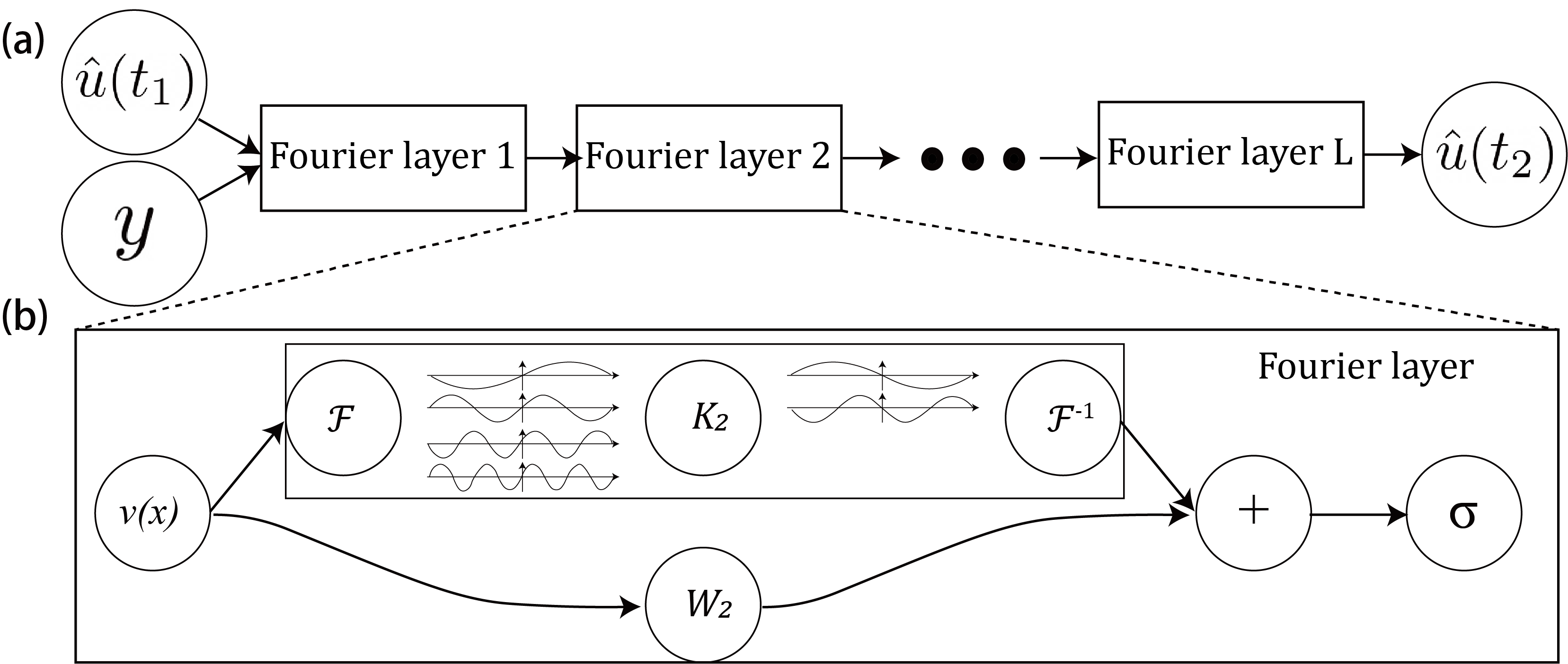
As shown in Figure 1, the neural operator [23] composes linear integral operator with pointwise non-linear activation function to approximate highly non-linear operators.
| (1) |
where , are the pointwise neural networks that encode the lower dimension function into higher dimensional space and vice versa. The model stack layers of where are pointwise linear operators (matrices), are integral kernel operators. We use ReLU activation in all numerical experiments, where element-wise. The parameters of the neural operator to be learned consists of all the parameters in .
In the Fourier neural operator (FNO) [23], the integral kernel operators are restricted to convolution, and implemented with Fourier transform:
| (2) |
where denotes the Fourier transform of a function , denotes its inverse, and denotes the linear transformation matrix applied to function in Fourier domain. An illustration is given in Figure 1.
Leveraging FNO’s powerful representation ability and superior computation efficiency, we propose to use it for learning and accelerating PDE observer computations. As we show here through our experiment results, FNO achieves up to three orders of magnitude improvement in computational speed compared to traditional PDE solvers, making FNO-PDE observers suitable for real-time control and monitoring.
III METHODS
In this section, we describe the proposed ML-accelerated PDE backstepping observers. We start with introducing the structure of a Learning-type PDE observer; we then present two model structures for implementation.
III-A A PDE observer with boundary sensing
We consider a general nonlinear PDE system on a 1-D spatial interval ,
| (3) |
where denotes the system state, whose arguments will be suppressed wherever possible for the sake of legibility. are real-valued functions of the state, and assume is differentiable over the state space. Suppose the boundary value is available for measurement.
We formulate a Luenberger-type PDE observer
| (4) |
where the first three terms are a copy of the system (3) and is a gain function of the observer, to be designed (typically using the PDE backstepping approach). Denoting the state estimation error and subtracting (4) from (3), we get the observer error system
| (5) |
where and is defined, using the mean value theorem, through .
The goal of observer design is for the estimation error to converge to zero as time goes to infinity, with respect to a particular spatial norm. This is to be achieved by making the origin of the PDE (III-A) exponentially stable through the choice of the observer gain function . Using the PDE backstepping approach [1], such a stabilizing can be found, under suitable conditions on the functions (e.g., for constant and linear , but also much more generally) and on the regularity of the observer initial error.
To obtain the state estimate in real time, one needs to simulate the observer (4) in real time. This observer is a PDE itself, with as its input. The PDE (4) does not have an explicit solution in general, and numerically generating its solution may be prohibitively slow for certain real-time applications such as for feedback control.
III-B ML-accelerated PDE backstepping observers
Motivated by the challenges highlighted above, the question we address in this paper is:
Can we use machine learning to design computationally-efficient PDE observers while maintaining rigorous performance guarantees in state estimation?
We answer the question affirmatively by designing an ML-accelerated PDE observer framework that learns a functional mapping from the initial observer state and system boundary measurements, to the state estimation. To guarantee the convergence of the neural observer to the state of the actual PDE system, we generate supervised training data from PDE observers designed by the backstepping method. To accelerate the computational efficiency, we use FNO for model learning, which shows superior performance in learning mappings between infinite-dimensional spaces of functions. Pairing the PDE backstepping design of observer gains with an FNO approximation of the observer PDEs resulting from backstepping inherits the mathematical rigor of the former (backstepping) and the computational performance of the latter (FNO)—allowing us to achieve the best of both worlds.
Specially, we propose two types of ML-accelerated PDE observers, i) the Feedforward Neural Observer, which learns the mapping from the initial state and the entire sequence of system boundary measurements, to the state estimation; and ii) the Recurrent Neural Observer, which learns a mapping from the previous step’s state estimation and boundary measurement to the next time step’s state estimation. The learned mapping is then applied recursively over the temporal domain to obtain the overall state estimation.
III-B1 Feedforward Neural Observer
Consider a time horizon with a measurement interval and contains intervals: . Here and hereafter, we use to denote the entire system operation horizon, the time interval between two measurements, and the total number of measurements. For the feedforward neural observer design, we learn a neural operator that directly maps the initial estimate and system measurements to the estimates . Figure 2 illustrates the model structure of this direct prediction approach.
III-B2 Recurrent Neural Observer
Unlike the first approach where inputs over time are fed into the neural operator as a full vector, the recurrent approach feeds input sequentially. At time step , it uses the previous step state estimate , and the input to obtain the current timestep state estimate via the following computation:
where is the neural operator. The state estimate is passed into the neural operator at time with the same parameters. Figure 3 shows the model structure of the recurrent neural observer.


Comparing the two model structures, we observed that the feedforward neural observers tend to obtain better estimation accuracy and train faster compared to their recurrent-structured counterparts in simulations, which is suitable for smoothing process where the neural observer is given the observations on a time interval to estimate the solution on the interval. On the other hand, the recurrent neural observer produces system estimation at each timestep, it can be applied to applications of observer-based controllers.
IV EXPERIMENTS
To illustrate the capability of the proposed ML-accelerated PDE observers, we compare the proposed observers with the conventional PDE observer on a chemical tubular reactor example (nonlinear parabolic PDEs) with both an exponential convergent backstepping observer and a prescribed-time convergent backstepping observer, and a backstepping traffic observer (nonlinear hyperbolic PDEs).
In order to demonstrate the effectiveness of FNO-backstepping pairing, we add a baseline long short-term memory (LSTM) model, which is a commonly used deep learning model capable of learning dependence in sequence prediction. Unless otherwise specified, we use training instances and 100 testing instances. We use Adam optimizer to train for 500 epochs222Number of epochs defines the number times that the learning algorithm will work through the entire training dataset. with an initial learning rate of that is halved every 100 epochs. Both the recurrent neural operator and LSTM are trained with the teacher-forcing [24] that takes ground truth values as supervision during training.
IV-A Exponentially Convergent Observer for a Reaction-Diffusion PDE
We start with a chemical tubular reactor system, the dynamics of which are represented as,
| (6a) | ||||
| (6b) | ||||
where is the temperature, , and . Equations (6a) and (6b) describe the heat transfer process within a heat generation chemical reaction [1]. The coefficient function is a “one-peak” function, where the peak location and value are controlled by and . We use second, in the experiments. The open-loop system is unstable with , which makes the estimation problem challenging.
A backstepping observer for system (6) is given by [1]
| (7a) | ||||
| (7b) | ||||
with the backstepping gain function
| (8) |
The exponential convergence of this observer is guaranteed by [1, Theorem 8].
To measure the performance of the model, we use the relative L2 error defined as follows,
where is the state estimation from the backstepping PDE observer in Eq (7) and (8) for test instance , and is the state estimation from the learning based observers.
Table I shows that training and test error of three ML-accelerated observers. Both neural operators perform significantly better than the LSTM model. We further compare the computation efficiency of the ML-accelerated observers against the backstepping PDE observers. As evident from Table II, the ML-accelerated observers achieve significant speedup compared to the classic finite-difference PDE solver. In particular, the feedforward neural observer can shorten the computation time by more than three orders of magnitude, while maintaining accurate state estimation.
| Model | Feedforward Neural Observer | Recurrent Neural Observer | LSTM |
| Parameters | 2,368,033 | 549,633 | 4,917,101 |
| Total Training Time (Hours) | 0.37 | 4.45 | 0.069 |
| Training Error | 7.28e-4 | 2.95e-3 | 0.466 |
| Test Error | 5.68e-4 | 0.1903 | 0.595 |
In addition to the significant acceleration of the neural observers compared to conventional PDE observers, we also hope to point out that the “price” is being paid in terms of upfront computation cost. On the one hand, to train the neural observers, we need to generate training data via conventional solvers. For example, we collected 1000 training data with a finite-difference solver given different initial conditions, which accounts for h upfront computation time. In addition, the feedforward neural operator training takes 500 epochs and each epoch takes 2.64s which needs h total training time. For the recurrent neural operator, the per epoch training time is 32.05s and the total training time is h.
| Method | Time (seconds/instance) |
| Conventional PDE Observer | 7.76 |
| Feedforward Neural Observer | 0.0065 |
| Recurrent Neural Observer | 0.188 |
| LSTM | 0.0237 |
IV-B Prescribed-Time Observer for a Reaction-Diffusion PDE
In addition to the exponentially convergent observers, we demonstrate the performance of the ML-accelerated prescribed-time (PT) convergent observers. For the same chemical tubular reactor system in (6) with time-invariant coefficient , following [14, Proposition 5.3], the backstepping PDE observer is designed as,
| (9) |
which employs the boundary measurement and the time-varying backstepping gain function
| (10) | ||||
| (11) |
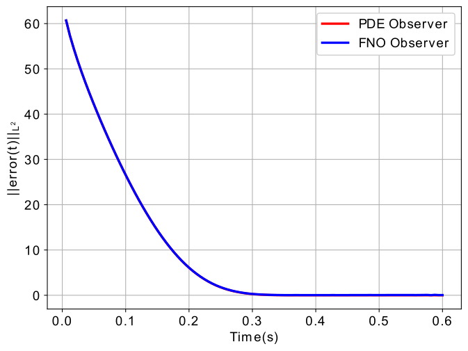
guarantees the convergence of to by , for arbitrarily short . This poses stringent requirements for the accuracy of neural observers since they’re required to obtain same prescribed-time convergence behavior.
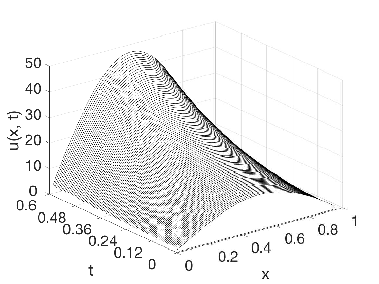
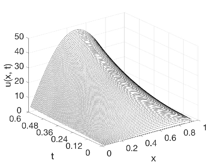
In the experiment, the reaction–diffusion equation (7) is defined with parameters and (constant), which is unstable without control input. The prescribed convergent time defined as second. For the backstepping PDE observer, we solve via an implicit Euler method with discretization and , and we approximate (10) by limiting its characterization to the first eight terms of their infinite series. Figure 4 shows that the true system dynamics, the PDE backstepping observer (9) and the feedforward neural observer for one test case. Table III compares the performance of different ML-accelerated observers and Table IV compares the computational efficiency. The acceleration with the feedforward neural observer is, again, about a thousandfold.

| Model | Feedforward Neural Observer | Recurrent Neural Observer | LSTM |
| Parameters | 2,368,033 | 549,633 | 4,440,048 |
| Total Training Time (Hours) | 0.24 | 2.42 | 0.067 |
| Training Error | 3.84e-4 | 2.51e-3 | 4.64e-4 |
| Test Error | 4.58e-4 | 9.05e-2 | 0.609 |
| Method | Time (seconds/instance) |
| Conventional PDE Observer | 11.308 |
| Feedforward Neural Observer | 0.0058 |
IV-C Traffic Flow PDE Observer
Finally, we demonstrate the performance of the ML-accelerated observers on a traffic problem. Traffic state estimation plays an important role in traffic control. Due to the technical and economic limitations, it is difficult to directly measure the system state everywhere thus it requires a traffic observer that can forecasting the system states with partially observed data.The traffic dynamics is described by the Aw–Rascle–Zhang (ARZ) PDEs model,
| (12a) | ||||
| (12b) | ||||
where the state variable denotes the traffic density and denotes the traffic speed. denotes the equilibrium speed-density relationship, a decreasing function of density.
The backstepping observer is designed in [19],
| (13a) | ||||
| (13b) | ||||
where is the freeway length, with boundary conditions
| (14) |
and the boundary measurement of the incoming traffic flow , outgoing velocity , and outgoing traffic flow , which appears in the output error injection terms and in (13). [19, Theorem 3] shows the observer design (13) guarantees exponential convergence. The numerical solution of the nonlinear ARZ PDEs and the nonlinear boundary observers are solved with the Lax–Wendroff method. For collecting the training and test data, we sample the reference density uniformly between vehicles/km, and reference velocity uniformly between [10, 12] m/s. Other parameters are the same as Table 1 in [19].
Performance comparison between different ML-accelerated observers are provided in Table V. We also compare the computational efficiency of the backstepping PDE observers in [19], which takes 0.839s to solve each instance, whereas the ML-accelerated method only takes 0.0051s for each instance, which achieves a hundredfold acceleration while keeping the high estimation accuracy.
| Model | Feedforward Neural Observer | Recurrent Neural Observer | LSTM |
| Parameters | 2,368,290 | 550,018 | 6,634,202 |
| Training Time (Hours) | 0.53 | 3.23 | 0.051 |
| Training Error | 5.23e-3 | 2.61e-2 | 1.04e-2 |
| Test Error | 5.51e-3 | 9.42e-2 | 1.78e-2 |
V CONCLUSIONS
We proposed an ML-accelerated PDE observer design framework which leverages the PDE backstepping design of observer gains and FNO for model learning. It highlights the benefits of inheriting the mathematical rigor of the PDE backstepping observers and obtain significant computational acceleration. We demonstrate the performance of the ML-accelerated observers in three benchmark PDE examples. There are many interesting open questions that remain. One important direction is to combine the ML-accelerated observers with downstream control tasks and study their real-time performance, especially in the presence of unmodeled PDE system disturbances.
References
- [1] A. Smyshlyaev and M. Krstic, “Backstepping observers for a class of parabolic pdes,” Systems & Control Letters, vol. 54, no. 7, pp. 613–625, 2005.
- [2] M. Krstic, B.-Z. Guo, A. Balogh, and A. Smyshlyaev, “Output-feedback stabilization of an unstable wave equation,” Automatica, vol. 44, no. 1, pp. 63–74, 2008.
- [3] ——, “Control of a tip-force destabilized shear beam by observer-based boundary feedback,” SIAM Journal on Control and Optimization, vol. 47, no. 2, pp. 553–574, 2008.
- [4] P. Bernard and M. Krstic, “Adaptive output-feedback stabilization of non-local hyperbolic pdes,” Automatica, vol. 50, no. 10, pp. 2692–2699, 2014.
- [5] F. Di Meglio, R. Vazquez, and M. Krstic, “Stabilization of a system of coupled first-order hyperbolic linear pdes with a single boundary input,” IEEE Transactions on Automatic Control, vol. 58, no. 12, pp. 3097–3111, 2013.
- [6] A. Hasan, O. M. Aamo, and M. Krstic, “Boundary observer design for hyperbolic pde–ode cascade systems,” Automatica, vol. 68, pp. 75–86, 2016.
- [7] J. Wang and M. Krstic, “Output feedback boundary control of a heat pde sandwiched between two odes,” IEEE Transactions on Automatic Control, vol. 64, no. 11, pp. 4653–4660, 2019.
- [8] ——, “Output-feedback control of an extended class of sandwiched hyperbolic pde-ode systems,” IEEE Transactions on Automatic Control, vol. 66, no. 6, pp. 2588–2603, 2021.
- [9] M. Krstic, B.-Z. Guo, and A. Smyshlyaev, “Boundary controllers and observers for the linearized schrödinger equation,” SIAM Journal on Control and Optimization, vol. 49, no. 4, pp. 1479–1497, 2011.
- [10] O. M. Aamo, A. Smyshlyaev, M. Krstic, and B. A. Foss, “Output feedback boundary control of a ginzburg–landau model of vortex shedding,” IEEE Transactions on Automatic Control, vol. 52, no. 4, pp. 742–748, 2007.
- [11] M. Krstic, L. Magnis, and R. Vazquez, “Nonlinear Control of the Viscous Burgers Equation: Trajectory Generation, Tracking, and Observer Design,” Journal of Dynamic Systems, Measurement, and Control, vol. 131, no. 2, 02 2009, 021012.
- [12] R. Vazquez and M. Krstic, “Boundary observer for output-feedback stabilization of thermal-fluid convection loop,” IEEE Transactions on Control Systems Technology, vol. 18, no. 4, pp. 789–797, 2010.
- [13] Vazquez, Rafael and Krstic, Miroslav, “Explicit output-feedback boundary control of reaction-diffusion pdes on arbitrary-dimensional balls,” ESAIM: COCV, vol. 22, no. 4, pp. 1078–1096, 2016.
- [14] D. Steeves, M. Krstic, and R. Vazquez, “Prescribed-time -stabilization of reaction-diffusion equations by means of output feedback,” in 2019 18th European Control Conference (ECC), 2019, pp. 1932–1937.
- [15] S. J. Moura, F. B. Argomedo, R. Klein, A. Mirtabatabaei, and M. Krstic, “Battery state estimation for a single particle model with electrolyte dynamics,” IEEE Transactions on Control Systems Technology, vol. 25, no. 2, pp. 453–468, 2017.
- [16] S. Koga, M. Diagne, and M. Krstic, “Control and state estimation of the one-phase stefan problem via backstepping design,” IEEE Transactions on Automatic Control, vol. 64, no. 2, pp. 510–525, 2019.
- [17] S. Koga and M. Krstic, “Arctic sea ice state estimation from thermodynamic pde model,” Automatica, vol. 112, p. 108713, 2020.
- [18] R. Vazquez, E. Schuster, and M. Krstic, “Magnetohydrodynamic state estimation with boundary sensors,” Automatica, vol. 44, no. 10, pp. 2517–2527, 2008.
- [19] H. Yu, Q. Gan, A. Bayen, and M. Krstic, “Pde traffic observer validated on freeway data,” IEEE Transactions on Control Systems Technology, vol. 29, no. 3, pp. 1048–1060, 2020.
- [20] J. Pathak, S. Subramanian, P. Harrington, S. Raja, A. Chattopadhyay, M. Mardani, T. Kurth, D. Hall, Z. Li, K. Azizzadenesheli et al., “Fourcastnet: A global data-driven high-resolution weather model using adaptive fourier neural operators,” arXiv:2202.11214, 2022.
- [21] J. Han, A. Jentzen, and E. Weinan, “Solving high-dimensional partial differential equations using deep learning,” Proceedings of the National Academy of Sciences, vol. 115, no. 34, pp. 8505–8510, 2018.
- [22] L. Lu, P. Jin, and G. E. Karniadakis, “Deeponet: Learning nonlinear operators for identifying differential equations based on the universal approximation theorem of operators,” arXiv:1910.03193, 2019.
- [23] Z. Li, N. B. Kovachki, K. Azizzadenesheli, B. liu, K. Bhattacharya, A. Stuart, and A. Anandkumar, “Fourier neural operator for parametric partial differential equations,” in International Conference on Learning Representations (ICLR), 2021.
- [24] A. M. Lamb, A. G. ALIAS PARTH GOYAL, Y. Zhang, S. Zhang, A. C. Courville, and Y. Bengio, “Professor forcing: A new algorithm for training recurrent networks,” Advances in neural information processing systems, vol. 29, 2016.