lsirm12pl: An R package for the latent space item response model
Abstract
The latent space item response model (LSIRM; Jeon et al. (2021)) allows us to show interactions between respondents and items in item response data by embedding both items and respondents in a shared and unobserved metric space. The R package lsirm12pl implements Bayesian estimation of the LSIRM and its extensions for different response types, base model specifications, and missing data. Further, the lsirm12pl offers methods to improve model utilization and interpretation, such as clustering of item positions in an estimated interaction map. lsirm12pl also provides convenient summary and plotting options to assess and process estimated results. In this paper, we give an overview of the methodological basis of LSIRM and describe the LSIRM extensions considered in the package. We then present the utilization of the package lsirm12pl with real data examples that are contained in the package.
Introduction
Item response theory (IRT) models are a widely used statistical approach to analyze assessment data in various research areas, such as medical, educational, psychological, health, and marketing research (An and Yung, 2014; Zanon et al., 2016). These models are designed to establish a relationship between observable item response data and unobservable person characteristics, commonly referred to as latent traits, e.g., competencies, attitudes, or personality (de Ayala, 2009; Brzezińska, 2018). IRT models can predict the probability of a correct (or positive) response as a function of the respondents’ latent traits and item features such as difficulty. The 2PL model includes an additional set of item parameters, called item discrimination parameters, which measure test items’ ability to discriminate between respondents with similar ability levels. Additional details of these models are described.
Several R packages are available for implementing IRT models. The ltm package (Rizopoulos, 2006) is available to analyze dichotomous and polytomous item response data, including the Rasch model, a two-parameter logistic model, a three-parameter model (Rasch, 1960; Birnbaum, 1968) and a graded response model (Samejima, 1968). The eRm package (Mair and Hatzinger, 2007) estimates various extensions of the Rasch model, such as the rating scale model (RSM) (Andrich, 1978), and the partial credit model (PCM) (Masters, 1982), linear logistic test model (LLTM) (Scheiblechner, 1972), the linear rating scale model (LRSM) (Fischer and Parzer, 1991), and the linear partial credit model (LPCM) (Glas and Verhelst, 1989; Fischer and Ponocny, 1994). The mirt package (Chalmers, 2012) can estimate a wide range of IRT models, including exploratory and confirmatory multidimensional item response models. The pcIRT package (Hohensinn, 2018) provides functions for estimating IRT models for polytomous (nominal) and continuous data, including the multidimensional polytomous Rasch model (Andersen, 1973) and the continuous rating scale model (Müller, 1987), using conditional maximum likelihood (CML) estimation (Baker and Kim, 2023). The brms package (Bürkner, 2021) offers various response distributions for Bayesian IRT models and models for reaction times or rates.
Conventional IRT models are typically based on two assumptions: conditional independence and homogeneity. Conditional independence assumes that item responses are independent of each other and conditional on respondents’ attributes. The homogeneity assumption is that respondents with the same ability have the same probability of answering a question correctly and that respondents have the same probability of answering a question with the same item difficulty. However, these assumptions are often violated in practice due to unobserved interactions between respondents and items, such as when particular items are more similar to each other (e.g., tests) or when particular respondents show different probabilities of giving correct responses to certain items compared to other respondents with similar ability (e.g., differential item functioning).
Jeon et al. (2021) proposed a latent space item response model (LSIRM) that addresses the limitations of conventional IRT models by introducing an interaction map, which embeds both items and respondents in a shared and unobserved metric space. This model allows for the interactions between respondents and items as distances between the latent positions of items and respondents. The probability of a correct response is modeled as a function of the distance between the respondent and the item’s latent positions in the latent space, given the respondent’s ability and the item’s difficulty. In addition to addressing the assumptions of conditional independence and homogeneity, the LSIRM approach provides useful diagnostic information on both items and respondents.
This paper presents the lsirm12pl package in R that offers Bayesian estimation of the LSIRM and its extensions. Jeon et al. (2021) focused on binary item response data and the Rasch model as the base model, and currently no package is available for estimating LSIRMs. To broaden the applicability of latent space item response modeling, lsirm12pl enables: (1) modeling continuous item responses; (2) missing data handling under different missing mechanisms assumptions (Rubin, 1976); and (3) an extended base model specification using the 2PL model both for binary and continuous item response data. A function to visualize unobserved interactions between items and respondents in a two-dimensional latent space, the package provides options to cluster latent item positions in the estimated interaction map. Details of the clustering methods are described in Section 0.3.2. lsirm12pl provides convenient summary and plotting options for model assessment, diagnosis, and result process and interpretation, which improves the utilization of LSIRMs in practice.
The subsequent sections of the paper are structured as follows. To begin, we will provide a concise overview of the 1PL and 2PL IRT models. Following that, we will delve into the LSIRM for binary response data and demonstrate how to fit the model with package functions using a real dataset. Moreover, we extend LSIRM to accommodate continuous data and provide guidance on fitting this extended model using the lsirm12pl package. In the end, we’ll conclude the paper with our final remarks and a discussion on future developments.
Item Response Models
1PL IRT Model
The 1PL model, also known as the Rasch model (Rasch, 1961), is a classical IRT model for analyzing dichotomous item response data. Suppose is the binary item response matrix under analysis, where indicates a correct (or positive) response of the -th respondent to the -th item. In the Rasch model, the probability of the correct response for item given by respondent is given as follows:
| (1) |
where is the respondent intercept parameter of respondent , is the item intercept parameter of item . The person intercept parameter represents the latent trait of interest, such as cognitive ability. The item intercept parameter represents the item easiness (or minus difficulty). As the respondent’s ability increases, the likelihood of giving correct responses increases. On the other hand, the likelihood of correct responses decreases as the difficulty of the item increases.
2PL IRT Model
The 2PL model (Birnbaum, 1968) extends the 1PL model by incorporating a discrimination parameter for each item. This parameter reflects the ability of the item to differentiate among respondents with similar abilities. The item discrimination parameters can also be considered as item slopes, indicating how quickly the probability of correct responses increases as the respondent’s abilities increase (An and Yung, 2014). A larger discrimination parameter indicates that the item is better at distinguishing between respondents with similar ability levels. In the 2PL model, the probability of person giving a correct response to item is given as follows:
| (2) |
where is the discrimination parameter for the item .
As we mentioned earlier, two assumptions about the IRT model, conditional independence and homogeneity, are often violated in practice. To address these issues, Jeon et al. (2021) proposed LSIRM. In the following sections, we describe the LSIRM and its applications.
1PL LSIRM For Dichotomous Data
Statistical framework
Consider the binary item response matrix , where is a response of the -th respondent to the -th item. Let indicate a correct response of the respondent to item , while indicates an incorrect response. To capture unobserved interactions between respondents and items and to alleviate the conditional independence and homogeneity assumptions of conventional IRT models, the original LSIRM (Jeon et al., 2021) extends the Rasch model (Rasch, 1961) by introducing -dimensional latent Euclidean space into the Rasch model. The -dimensional latent Euclidean space, called an interaction map, captures and represents pairwise interactions between respondents and items. The original LSIRM involves a single set of item parameters, item intercepts; thus, we refer to it as the one-parameter logistic LSIRM (1PL LSIRM).
The 1PL LSIRM assumes that the probability of giving a correct answer to item by the respondent is determined by a linear combination of the main effect of the -th respondent, the main effect of the -th item, and the pairwise distance between the latent position of item and the latent position of respondent . Then, the model is given by:
| (3) |
where , , , and are the main effect of the respondent , the main effect of the item , the latent position of the respondent , and the latent position of the item , respectively. The pairwise distance is calculated using a distance function , where we use a Euclidean norm (that is, ) as a distance function in lsirm1pl. The distance weight captures the degree of deviations from the main effects of the Rasch model, and a higher value of indicates stronger evidence or a greater need to add the interaction term .
The likelihood function of the observed data with the 1PL LSIRM is
| (4) |
where , , and . Here, item responses are assumed to be independent conditional on the positions of respondents and items in an interaction map, as well as the main effects of respondent and item, alleviating the traditional conditional independence assumption. The detailed parameter estimations are described in the following Section.
The lsirm12pl package uses a fully Bayesian approach using the Markov chain Monte Carlo (MCMC) for estimation.
An Illustrated Example
In this section, we demonstrate how to apply the 1PL LSIRM to real datasets using the lsirm12pl package. To illustrate the method, we used the Inductive Reasoning Developmental Test (TDRI) dataset (Golino, 2016), which contains item responses from 1,803 Brazilians (52. 5% female) of ages ranging from 5 to 85 years (M = 15.75; SD = 12.21). TDRI is a pencil-and-paper test consisting of 56 items that are designed to assess developmentally sequenced and hierarchically organized inductive reasoning. The dataset is publicly available for reproducibility purposes and can be downloaded from the following link:
https://figshare.com/articles/dataset/TDRI_dataset_csv/3142321.
The lsirm12pl package provides several functions for conducting the LSIRM, which require hyperparameter values for prior distributions and/or tuning parameters for MCMC chains. By default, the lsirm function runs with the default settings unless these values are specified by the user. The default MCMC run setting includes 15,000 iterations, 2,500 burn-in, and 5 thinning, and the parameter values of the corresponding items are printed every 500 iterations. The base function for LSIRM is
lsirm(A <term 1>(<term 2>, <term 3>, ...))
where A is a binary or continuous item response matrix to be analyzed, <term1> could be either ‘lsirm1pl’ or ‘lsirm2pl’, and <term 2>, <term 3> are specific options for the model, which are explained in the documentation of the lsirm12pl package. Following is the practical example of fitting 1PL LSIRM to the TDRI dataset without any missing values. We fit the model with the default setting by set by leaving <term 2> blank. Detailed explanations of these default settings can be found within the documentation of the lsirm12pl package.
R > set.seed(2023)R > library("lsirm12pl")R > data <- lsirm12pl::TDRIR > data <- data[complete.cases(data),]R > lsirm_result <- lsirm(data ~ lsirm1pl())
The estimation results for the parameters and are presented in a list format, with additional summary information provided by the summary() function. This function provides the MCMC sample size and options, posterior means of the covariate coefficients (), the overall Bayesian information criterion (BIC) and the maximum logarithmic posterior value.
R > summary(lsirm_result)==========================Summary of model==========================Call: lsirm.formula(formula = data ~ lsirm1pl())Model: lpl LSIRMData type: binaryVariable Selection: FALSEMissing: NAMCMC sample of size 15000, after burnin of 2500 iterationCovariate coefficients posterior means: Estimate 2.5% 97.5%i1 6.44692 5.83577 7.1210...i56 -1.13026 -2.50031 0.5180---------------------------Overall BIC (Smaller is better) : 43675.26Maximum Log-posterior Iteration: value iter[1,] -11508 1202
The function diagnostic() allows us to check the convergence of MCMC for each parameter with various diagnostic plots, such as trace plots, autocorrelation functions (ACF), and posterior density distributions. The options of the diagnostic() function are which.draw and draw.item. These two options refer to the names and indexes of the parameters to diagnose, respectively. Figure 1 displays the output of diagnostic() for by setting the options to which.draw = c("beta"), draw.item = list("beta" = c(1)). The same diagnostic plots can be applied to other parameters.
R > diagnostic(lsirm_result, which.draw = c("beta"), draw.item = list("beta" = c(1)))

The lsirm12pl package offers the gof() function, which allows users to assess the goodness of fit of LSIRM to the observed item response data. Main diagnostic tool is a boxplot that displays the average posterior predicted response value for each item. The average observed response value for each item is indicated by red dots. When the model fits well, the red dot is close to the midline of the boxplot. The number of posterior predictive samples for drawing a boxplot can be adjusted by the user using the nsim option.
In the case of binary item response data, the gof() function in the LSIRM package includes a receiver operating characteristic (ROC) curve to assess the performance of LSIRM. Figure 2 presents the output of the gof() function for the TDRI dataset, presenting both the boxplot and the ROC curve. In this example, all of the red dots are closely located at the midline of the boxplot and the area under the curve (AUC) of the ROC curve approaches 1, suggesting that the fit of the LSIRM to the data is satisfactory.
R > gof(lsirm_result, nsim = 500)
 |
Users can utilize the plot() function to generate a variety of plots based on LSIRM results. For example, with the "beta" option, the function generates boxplots of posterior samples for the item main effect parameter, . With the "theta" option, we can generate boxplots of the point estimates for , which are plotted against the total sum scores of positive responses (ranging from 0 to ).
Figures 3 illustrate the results for plot() with options "beta" and "theta", respectively. In Figure 3(a), the outliers are suppressed in the boxplot for the sake of simplicity.
R > plot(lsirm_result, option = "beta")R > plot(lsirm_result, option = "theta")


Finally, the "interaction" option is used to visualize the interaction map, which displays the point estimates of the latent positions of the respondents and the items on a two-dimensional map. The primary and unique advantage of LSIRM lies in providing intuitive inference based on an interaction map, which visualizes unobserved interactions between items and respondents. The dimension of the latent space is set to a two-dimensional space, which was adopted by Jeon et al. (2021) for parsimony and interpretability.
The interaction map represents item-by-person interactions as distances between respondents and items. A shorter distance between the latent position of the -th item () and the latent position of the -th respondent () indicates a stronger dependence (or interactions), which in turn implies that the respondent is more likely to respond correctly (or positively) to the item . Figure 4(a) shows the interaction map based on the 1PL LSIRM for the TDRI data. In Figure 4(a), the latent positions of most respondents are spread around the center of the interaction map, while the item latent positions are separated, revealing roughly four clusters. For example, the item cluster on the right red box and bottom red box appears apart from most respondents on the map. This suggests that most respondents were likely to respond incorrectly to items in this item cluster, regardless of their ability levels.
If desired, the interaction map can be rotated to improve the interpretability of the coordinates of the map. The lsirm12pl package offers the oblimin rotation (Jennrich, 2002) using the GPArotation package in R (Bernaards and Jennrich, 2005). Figure 4(b) is the rotated version of the original map shown in Figure 4(a). In this example, the original and rotated maps are similar in terms of the item configuration, because the items are already being placed close to the two coordinates in Figure 4(a).
R > plot(lsirm_result, option = "interaction")R > plot(lsirm_result, option = "interaction", rotation = T)


The lsirm12pl package also offers the option to cluster item latent positions. Two types of clustering methods are available: spectral clustering (Ng et al., 2001; von Luxburg, 2007) and the Nayman-Scott process modeling approach (Thomas, 1949; Neyman and Scott, 1952; Yi et al., 2023), with spectral and neyman options, respectively. For spectral clustering, the implementation is based on the specc package (Karatzoglou et al., 2004) in R and the number of clusters is determined using the average silhouette width (Batool and Hennig, 2021). For the Neyman-Scott process modeling approach, the lsirm12pl package applies the MCMC algorithm 100 times to obtain the center and a number of clusters and then assigns items to the nearest cluster based on the Euclidean distances.
The results based on spectral clustering and the Neyman-Scott process model are shown below on the R console. Figure 5(a) displays the result of the spectral clustering method and Figure 5(b) illustrates that of the Neyman-Scott process model. In both figures, the gray dots and numbers represent the latent positions of the respondents and the items simultaneously, where the color of the numbers indicates the cluster membership. The Neyman-Scott process model additionally displays the center of the item cluster using alphabets and a contour for each item cluster. In this example, the result of the Neyman-Scott process model shows more clusters compared to the spectral clustering method.
R > plot(lsirm_result, cluster = "spectral")R > plot(lsirm_result, cluster = "neyman")Clustering result (Spectral Clustering): group item A 41, 42, 43, 44, 45, 46, 47, 48 B 49, 50, 51, 52, 53, 54, 55, 56 C 25, 26, 27, 28, 29, 30, 31, 32 D 33, 34, 35, 36, 37, 38, 39, 40 E 1, 2, 3, 4, 5, 6, 7, 8, 9, 10, 11, 12, 13, 14, 15, 16, 17, 18, 19, 20, 21, 22, 23, 24|==================================================| 100%Clustering result (Nayman-Scott process): group item A 25, 26, 27, 28, 29, 30, 31, 32 B 41, 42, 43, 44, 45, 46, 47, 48 C 7, 9, 10, 11, 12, 13, 14, 15, 16 D 1, 2, 3, 4, 5, 6, 8 E 50, 51, 53, 56 F 17, 18, 19, 20, 21, 22, 23, 24 G 33, 34, 35, 36, 37, 38, 39, 40 H 49, 52, 54, 55


Flexible Modeling Options
The lsirm12pl package provides a range of flexible modeling options for LSIRM. One such option is the ability to fix the distance weight to a constant value of 1. By doing so, the scale of the latent space can be standardized, making it easier to compare different interaction maps. To implement this option, the main function offers a Boolean input called fixed_gamma, which can be set to TRUE or FALSE depending on whether or not the distance weight is to be fixed. The default value of fixed_gamma is FALSE. The following is the example code for fitting the 1PL LSIRM with a fixed by specifying fixed_gamma as TRUE.
R > lsirm_result <- lsirm(data ~ lsirm1pl(fixed_gamma = TRUE))
Another option the lsirm12pl package offers is the spike-and-slab prior for the distance weight . This option allows us to determine whether is zero or not, which in turn determines whether the classical Rasch model is sufficient or whether interactions between respondents and items should be investigated using the LSIRM approach. If is zero, the classical Rasch model is sufficient, whereas if is not zero, it would be useful to investigate interactions between respondents and items with the LSIRM approach. The spike-and-slab prior is included in the package as an option with spikenslab.
The model selection between the Rasch model and the LSIRM can be based on the posterior probability of being non-zero, as indicated by the return value of pi_estimate. A pi_estimate value greater than 0.5 indicates that the data contain nonignorable interactions between the items and the respondents, and the LSIRM framework can be used to investigate these interactions. It is important to note that the two options fixed_gamma and spikenslab cannot be used at the same time as they determine the specification of .
R > lsirm_result <- lsirm(data ~ lsirm1pl(spikenslab = TRUE))R > lsirm_result[,"pi_estimate"][1] 0.9988
The lsirm12pl package also provides two options for handling missing data using the missing_data. If missing_data is set to "mcar", it is assumed that the data follow completely missing data at random mechanism (MCAR) (Rubin, 1976) and the parameters are estimated based solely on the observed elements of the dataset being analyzed. On the other hand, if missing_data is "mar", the data is assumed to be missing at random (MAR), and the data augmentation algorithm (Tanner and Wong, 1987) is applied to impute missing values. Since the option "mar" imputes missing values, the function returns the posterior samples of the imputed responses with imp and the probability of a correct response with imp_estimate. Imputed values are listed in the order of respondents. missing_data can be used in combination with other options such as (spikenslab = TRUE, missing_data = "mar"). Note that all missing values should be recoded via missing.val and the default value is 99. We replaced the missing values in the TDRI dataset with the value 99.
R > data <- lsirm12pl::TDRIR > data[is.na(data)] <- 99R > lsirm_result <- lsirm(data ~ lsirm1pl(missing_data = "mcar"))R > lsirm_result <- lsirm(data ~ lsirm1pl(missing_data = "mar"))R > lsirm_result[,"imp_estimate"][1] 0.9980 0.9900 0.9756 0.9800 0.9608 0.9628...[997] 0.9936 0.9780 0.8304 0.9892 [ reached getOption("max.print") -- omitted 32327 entries ]R > plot(lsirm_result, option = "interaction")
Figures 4(c) and 4(d) show the resulting interaction maps with both MAR and MCAR assumptions, respectively. In the current example, the interaction maps estimated using the two missing assumptions produced comparable results. If the interaction maps of two missing assumptions are significantly different, further investigation is necessary to determine which assumption would be more suitable for the analyzed data.
In particular, the interaction maps shown in Figures 4(c) and 4(d) are pretty similar to the original map presented in Figure 4(a). The original interaction map used complete item response data, whereas maps based on various missing assumptions were created from the original data, including respondents with missing item responses. The similarity between these maps suggests that the complete item response data provide a reasonable representation of the original item response data.
2PL LSIRM For Dichotomous Data
Ststistical framework
The two-parameter LSIRM (2PL LSIRM) builds upon the 1PL LSIRM by introducing the item discrimination parameters as shown in Equation (2). Specifically, the 2PL LSIRM models the probability of a correct response by respondent to item as follows:
where , , , and have similar interpretations as Equation (3). The observed data likelihood function under this model is given as
| (5) |
An Illustrated Example
In this section, we applied the 2PL LSIRM to the TDRI data which was used in the previous section. The default settings of 2PL LSIRM are the same as 1PL LSIRM except for . The base function for the 2PL LSIRM is
lsirm(A lsirm2pl())
This function returns a list of estimates on the model parameters, , , and .
R > set.seed(2023)R > library("lsirm12pl")R > data <- lsirm12pl::TDRIR > data <- data[complete.cases(data),]R > lsirm_result <- lsirm(data ~ lsirm2pl())
To diagnose the results of the 2PL LSIRM analysis, we can use the diagnostic() function. Figure 6 displays the diagnostic results for . These plots can help us assess the quality of the posterior sample and identify potential issues such as convergence problems.
R > diagnostic(lsirm_result, which.draw = c("beta"), draw.item = list(beta = c(1)))

The gof() function assesses the goodness-of-fit of the 2PL LSIRM. A comprehensive description of this function is provided in the 1PL LSIRM description. Figure 7 visualizes the boxplot and the ROC curve to check the model performance. In the figure, most of the red dots are located close to the midline of the boxplots and the AUC is 0.97, indicating that the model fits the TDRI dataset reasonably well.
R > gof(lsirm_result, nsim = 500)
 |
The visualization function plot() can be used again to summarize the estimated results and draw the interaciton map for 2PL LSIRM. The options for this function have been expanded by including the option to draw a boxplot for as well as the options discussed in the 1PL LSIRM description. Figure 8 illustrates the results of the plot() function with the "beta", "theta", and "alpha" options for the 2PL LSIRM.
R < plot(lsirm_result, option = "beta")R < plot(lsirm_result, option = "theta")R < plot(lsirm_result, option = "alpha")


We can use the plot() function with the "interaction" option to create a visualization of the interaction map based on the estimated results from the 2PL LSIRM. Figures 9(a) and 9(b) display the original and rotated interaction map, respectively. Although the interaction map based on the 2PL LSIRM is generally similar to the interaction map generated using the 1PL LSIRM in terms of item configuration, there may be some subtle differences. These differences may arise because the 2PL LSRIM includes item discrimination parameters, which can explain some degree of item-by-person interactions that are not captured by the 1PL LSIRM.
R < plot(lsirm_result, option = "interaction")R < plot(lsirm_result, option = "interaction", rotation = TRUE)


Figure 10(a) and 10(b) represent the result of spectral clustering and the Neyman-Scott process model, respectively. The interpretation of gray dots, numbers, alphabets, and contours is the same as in the results shown in the 1PL LSIRM.
R > plot(lsirm_result, cluster = "spectral")R > plot(lsirm_result, cluster = "neyman")Clustering result (Spectral Clustering): group item A 1, 2, 3, 4, 5, 6, 7, 8, 9, 10, 11, 12, 13, 14, 15, 16 B 33, 34, 35, 36, 37, 38, 39, 40 C 17, 18, 19, 20, 21, 22, 23, 24 D 25, 26, 27, 28, 29, 30, 31, 32 E 41, 42, 43, 44, 45, 46, 47, 48, 49, 50, 51, 52, 53, 54, 55, 56|==================================================| 100%Clustering result (Nayman-Scott process): group item A 9, 10, 11, 12, 13, 14, 15, 16 B 25, 26, 27, 28, 29, 30, 31, 32 C 41, 42, 43, 44, 45, 46, 47, 48 D 17, 18, 19, 20, 21, 22, 23, 24 E 33, 34, 35, 36, 37, 38, 39, 40 F 1, 2, 3, 4, 5, 6, 7, 8 G 49, 50, 51, 52, 53, 54, 55, 56


The modeling options discussed in Section 0.3.3 are available for the 2PL LSIRM. fixed_gamma fixes the distance weight to 1 and spikenslab assigns a spike and slab prior to . Additionally, the two missing data options, missing_data = "mcar" and missing_data = "mar", are also applicable for the 2PL LSIRM.
R > lsirm_result <- lsirm(data ~ lsirm2pl(fixed_gamma = TRUE))R > lsirm_result <- lsirm(data ~ lsirm2pl(spikenslab = TRUE))R > lsirm_result <- lsirm(data ~ lsirm2pl(missing_data = "mcar"))R > lsirm_result <- lsirm(data ~ lsirm2pl(missing_data = "mar"))
LSIRM For Continuous Item Responses Data
Ststistical framework
We consider an extension of the original LSIRM for continuous item response data (LSIRM-continuous), which can be done by using an appropriate link function following the generalized linear model framework (McCullagh and Nelder, 2019). Consider the continuous item response data consisting of the matrix . By choosing the identity link function for continuous item responses, the 1PL LSIRM-continuous is given as follows:
where and are the main effects of the respondent and the item , respectively. and are the latent positions of the respondent and the item , respectively. An additional error term explains unexplained residuals in the 1PL LSIRM-continuous. In other words, the model specifies that follows a normal distribution with mean and variance . A shorter distance between and indicates that the respondent is likely to give a higher response value to item given the main effects of the respondent and the item.
It is straightforward to extend the 1PL LSIRM-continuous to the 2PL version by adding item discrimination parameters . The 2PL LSIRM-continuous for is given as follows:
The interpretations of the model parameters in the 2PL LSIRM-continuous are similar to the case of the 1PL LSIRM-continuous and the 2PL LSIRM.
The likelihood function of the 1PL LSIRM-continuous is given as
and the likelihood function of the 2PL LSIRM-continuous is given as
An Illustrated Example
We demonstrate the application of LSIRM-continuous using the Big Five Personality Test dataset111The dataset can be downloaded for reproducible purposes from the following link: https://www.kaggle.com/tunguz/big-five-personality-test. Data were collected from 1,015,342 respondents using an interactive online personality test from 2016 to 2018. The “Big-Five Factor Markers” from the international personality item pool were used in the test, which consists of 50 questions with response categories 1 = disagree, 3 = neutral, and 5 = agree based on a five-point Likert scale. Negatively worded items were reverse-coded. For illustration purposes, we randomly selected a sample of 3,000 respondents from the original data. We treated the ordinal item responses as continuous data, which is a common practice in applied research and is generally considered acceptable for other models, such as factor analysis.
The function for the 1PL and 2PL LSIRM-continuous is identical to the 1PL and 2PL LSIRM for binary data. This is because the function automatically identifies the data type. Following is the code for data pre-processing and 1PL LSIRM-continuous fitting.
R > set.seed(2023)R > data <- lsirm12pl::BFPTR > data[(data==0)|(data==6)] = NAR > reverse <- c(2, 4, 6, 8, 10, 11, 13, 15, 16, 17, 18, 19, 20, 21, 23, 25, 27, 32, 34, 36, 42, 44, 46)R > data[, reverse] <- 6 - data[, reverse]R > data <- data[complete.cases(data),]R > lsirm_result <- lsirm(data ~ lsirm1pl(jump_beta = 0.08, jump_theta = 0.3))
To ensure convergence of the parameters in this example, different jumping rules are applied in this example. The estimated results are returned in the list containing estimated information on and . The functions summary(), diagnostics() and gof() described in 1PL LSIRM can be used to obtain a summary, diagnosis, and goodness-of-fit results.
 |
Figure 11 displays the diagnostic results for obtained by using the diagnostic() function.
R > diagnostic(lsirm_result, which.draw = c("beta"), draw.item = list(beta = c("AGR1")))
The result displayed in Figure 12 pertains to the goodness-of-fit assessment for continuous example data. Unlike binary data, ROC is not available for continuous data, so the results of the gof() function include only the boxplots of the average predicted response values. In this example, the red dots are located close to the midlines of the boxplots, implying a satisfactory model fit.
R > gof(lsirm_result, nsim = 500)
 |
The visualization function plot can be used to summarize the results.
R < plot(lsirm_result, option = "beta")R < plot(lsirm_result, option = "theta")
Figure 13(a) shows the box plots of the posterior samples for and Figure 13(b) shows the boxplots of the point estimates for .


Figure 14(a) illustrates the interaction map derived from the 1PL LSIRM-continuous. The distance between the latent position of the respondent and the item is large, the respondent is more likely to give a low response value to the item.
R < plot(lsirm_result)R < plot(lsirm_result, rotation = TRUE)
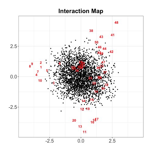

Figure 15(a) and Figure 15(b) depict the result of spectral clustering and the Neyman-Scott process model for the BFPT example dataset, respectively. Gray dots, numbers with colors, alphabets, and contours have the same interpretations as the clustering results presented in 1PL LSIRM result. The clustering results of both methods are identical in this example.
R > plot(lsirm_result, cluster = "spectral")R > plot(lsirm_result, cluster = "neyman")Clustering result (Spectral Clustering): group item A 1, 2, 3, 4, 5, 7, 8, 9, 10 B 38, 41, 42, 43, 44, 45, 46, 48, 49, 50 C 6, 21, 22, 24, 25, 26, 27, 28, 29, 30 D 23, 31, 32, 33, 34, 35, 36, 37, 39, 40, 47 E 11, 12, 13, 14, 15, 16, 17, 18, 19, 20|==================================================| 100%Clustering result (Nayman-Scott process): group item A 11, 12, 13, 14, 15, 16, 17, 18, 19, 20 B 1, 2, 3, 4, 5, 7, 8, 9, 10 C 6, 21, 22, 24, 25, 26, 27, 28, 29, 30 D 23, 31, 32, 33, 34, 35, 36, 37, 39, 40, 47 E 38, 41, 42, 43, 44, 45, 46, 48, 49, 50


Various flexible modeling options discussed in 1PL LSIRM can be applied to functions for LSIRM-continuous.
R > lsirm_result <- lsirm(data ~ lsirm1pl(fixed_gamma = TRUE))R > lsirm_result <- lsirm(data ~ lsirm1pl(spikenslab = TRUE))R > lsirm_result <- lsirm(data ~ lsirm1pl(missing_data = "mcar"))R > lsirm_result <- lsirm(data ~ lsirm1pl(missing_data = "mar"))
Conclusion
In this paper, we introduced the R package lsirm12pl for estimating LSIRM (Jeon et al., 2021) and its extensions. The original LSIRM framework was proposed for binary item response data based on the 1PL IRT base model. To broaden its applicability, we extended the original framework to cover different response types and model specifications. Further, we added a number of useful options, e.g., for handling missing data, item clustering, and model assessment. A fully Bayesian approach was used for model estimation with a Metropolis-Hastings-within-Gibbs sampler. The lsirm12pl package offers default estimation settings for priors, jumping rules, number of iterations, burn-in, and thinning. The default estimation setting works reasonably well in a wide range of situations, but users can manually revise the estimation settings if desired. In addition, the package lsirm12pl offers convenient supplemental functions to evaluate, summarize, visualize, diagnose, and interpret the estimated results. We provided detailed illustrations of the package with real data examples available in the package. We hope that these illustrations guide researchers in using the lsirm12pl package for the analysis of their own datasets.
The R package lsirm12pl is our first step in making the LSIRM approach more applicable and usable in practice. The code is written using Rcpp (Eddelbuettel and François, 2011; Eddelbuettel, 2013; Eddelbuettel and Balamuta, 2018) and RcppArmadillo (Eddelbuettel and Sanderson, 2014) in R for efficient computation. For example, the computation time was 2.06 min for the first data example with 726 respondents and 56 test items with lsirm1pl. We will continue to update the package by incorporating additional modeling, data analysis, and visualization options to make the lsirm12pl package more useful in a wider range of situations.
Acknowledgement
We thank the editor, associate editor, and reviewers for their constructive comments. We also thank Dr. Won Chang for constructive comments on our work. This study was partially supported by the Basic Science Research Program through the National Research Foundation of Korea (NRF 2020R1A2C1A01009881 and RS-2023-00217705). Correspondence should be addressed to Ick Hoon Jin, Department of Applied Statistics, Department of Statistics and Data Science, Yonsei University, Seoul, Republic of Korea. Go, Park, and Kim are co-first authors.
References
- An and Yung (2014) X. An and Y. F. Yung. Item response theory: What it is and how you can use the IRT procedure to apply it. SAS Institute Inc, 10(4), 2014.
- Andersen (1973) E. B. Andersen. CONDITIONAL INFERENCE FOR MULTIPLE-CHOICE QUESTIONNAIRES. British Journal of Mathematical and Statistical Psychology, 26(1):31–44, 1973. doi: 10.1111/j.2044-8317.1973.tb00504.x.
- Andrich (1978) D. Andrich. A rating formulation for ordered response categories. Psychometrika, 43(4):561–573, 1978. doi: 10.1007/bf02293814.
- Baker and Kim (2023) F. B. Baker and S.-H. Kim, editors. Item response theory. Statistics: A Series of Textbooks and Monographs. Taylor & Francis, London, England, 2 edition, 2023.
- Batool and Hennig (2021) F. Batool and C. Hennig. Clustering with the average silhouette width. Computational Statistics & Data Analysis, 158:107190, 2021. doi: 10.1016/j.csda.2021.107190.
- Bernaards and Jennrich (2005) C. A. Bernaards and R. I. Jennrich. Gradient projection algorithms and software for arbitrary rotation criteria in factor analysis. Educational and Psychological Measurement, 65(5):676–696, Oct. 2005. doi: 10.1177/0013164404272507.
- Birnbaum (1968) A. L. Birnbaum. Some latent trait models and their use in inferring an examinee’s ability. Statistical theories of mental test scores, 1968.
- Brzezińska (2018) J. Brzezińska. Item response theory models in the measurement theory with the use of ltm package in r. Econometrics, 22(1):11–25, 2018. doi: doi:10.15611/eada.2018.1.01.
- Bürkner (2021) P.-C. Bürkner. Bayesian item response modeling in R with brms and stan. Journal of Statistical Software, 100:1–54, 2021. doi: 10.18637/jss.v100.i05.
- Chalmers (2012) R. P. Chalmers. mirt: A Multidimensional Item Response Theory package for the R Environment. Journal of Statistical Software, 48(6):1–29, 2012. doi: 10.18637/jss.v048.i06.
- de Ayala (2009) R. J. de Ayala. The theory and practice of item response theory. Methodology in the Social Sciences. Guilford Publications, New York, NY, 2009.
- Eddelbuettel (2013) D. Eddelbuettel. Seamless R and C++ Integration with Rcpp. Springer, New York, 2013. ISBN 978-1-4614-6867-7.
- Eddelbuettel and Balamuta (2018) D. Eddelbuettel and J. J. Balamuta. Extending R with C++: A brief introduction to Rcpp. The American Statistician, 72(1):28–36, 2018. doi: 10.1080/00031305.2017.1375990.
- Eddelbuettel and François (2011) D. Eddelbuettel and R. François. Rcpp: Seamless R and C++ integration. Journal of Statistical Software, 40(8):1–18, 2011. doi: 10.18637/jss.v040.i08.
- Eddelbuettel and Sanderson (2014) D. Eddelbuettel and C. Sanderson. Rcpparmadillo: Accelerating r with high-performance c++ linear algebra. Computational Statistics and Data Analysis, 71:1054–1063, March 2014. doi: 10.1016/j.csda.2013.02.005.
- Fischer and Parzer (1991) G. H. Fischer and P. Parzer. An extension of the rating scale model with an application to the measurement of change. Psychometrika, 56(4):637–651, 1991. doi: 10.1007/bf02294496.
- Fischer and Ponocny (1994) G. H. Fischer and I. Ponocny. An extension of the partial credit model with an application to the measurement of change. Psychometrika, 59(2):177–192, 1994. doi: 10.1007/bf02295182.
- Glas and Verhelst (1989) C. A. W. Glas and N. D. Verhelst. Extensions of the partial credit model. Psychometrika, 54(4):635–659, 1989. doi: 10.1007/bf02296401.
- Golino (2016) H. Golino. Tdri dataset.csv, 2016. URL https://figshare.com/articles/dataset/TDRI_dataset_csv/3142321/1.
- Hohensinn (2018) C. Hohensinn. pcirt: An r package for polytomous and continuous rasch models. Journal of Statistical Software, Code Snippets, 84(2):1–14, 2018. doi: 10.18637/jss.v084.c02.
- Jennrich (2002) R. I. Jennrich. A simple general method for oblique rotation. Psychometrika, 67(1):7–19, Mar. 2002. doi: 10.1007/bf02294706.
- Jeon et al. (2021) M. Jeon, I. H. Jin, M. Schweinberger, and S. Baugh. Mapping unobserved item–respondent interactions: A latent space item response model with interaction map. Psychometrika, pages 1–26, 2021. doi: 10.1007/s11336-021-09762-5.
- Karatzoglou et al. (2004) A. Karatzoglou, A. Smola, K. Hornik, and A. Zeileis. kernlab – an S4 package for kernel methods in R. Journal of Statistical Software, 11(9):1–20, 2004. doi: 10.18637/jss.v011.i09.
- Mair and Hatzinger (2007) P. Mair and R. Hatzinger. Extended Rasch Modeling: The eRm Package for the Application of IRT Models in R. Journal of Statistical Software, 20(9):1–20, 2007. doi: 10.18637/jss.v020.i09.
- Masters (1982) G. N. Masters. A rasch model for partial credit scoring. Psychometrika, 47(2):149–174, 1982. doi: 10.1007/bf02296272.
- McCullagh and Nelder (2019) P. McCullagh and J. A. Nelder. Generalized linear models. Routledge, 2019.
- Müller (1987) H. Müller. A rasch model for continuous ratings. Psychometrika, 52(2):165–181, 1987. doi: 10.1007/bf02294232.
- Neyman and Scott (1952) J. Neyman and E. L. Scott. A theory of the spatial distribution of galaxies. The Astrophysical Journal, 116:144 –163, 1952. doi: 10.1086/145599.
- Ng et al. (2001) A. Y. Ng, M. I. Jordan, and Y. Weiss. On spectral clustering: Analysis and an algorithm. In Proceedings of the 14th International Conference on Neural Information Processing Systems: Natural and Synthetic, NIPS’01, page 849–856, Cambridge, MA, USA, 2001. MIT Press.
- Rasch (1960) G. Rasch. Probabilistic models for some intelligence and attainment tests. Danish Institute for Educational Research, Copenhagen, 1960.
- Rasch (1961) G. Rasch. On general laws and the meaning of measurement in psychology. In Proceedings of the Fourth Berkeley Symposium on Mathematical Statistics and Probability, Volume 4: Contributions to Biology and Problems of Medicine, pages 321–333, Berkeley, Calif., 1961. University of California Press. URL https://projecteuclid.org/euclid.bsmsp/1200512895.
- Rizopoulos (2006) D. Rizopoulos. ltm: An R package for latent variable modeling and item response analysis. Journal of Statistical Software, 17(5):1–25, 2006. doi: 10.18637/jss.v017.i05.
- Rubin (1976) D. B. Rubin. Inference and missing data. Biometrika, 63(3):581–592, 1976.
- Samejima (1968) F. Samejima. Estimation of latent ability using a response pattern of graded scores1. ETS Research Bulletin Series, 1968(1):i–169, 1968. doi: 10.1002/j.2333-8504.1968.tb00153.x.
- Scheiblechner (1972) H. Scheiblechner. Das lernen und lösen komplexer denkaufgaben. Zeitschrift für experimentelle und angewandte Psychologie, 19:476–506, 1972.
- Tanner and Wong (1987) M. Tanner and W. Wong. The calculation of posterior distributions by data augmentation (with discussion). Journal of the American Statistical Association, 82:528–550, 1987.
- Thomas (1949) M. Thomas. A generalization of poisson's binomial limit for use in ecology. Biometrika, 36(1/2):18–25, 1949. doi: 10.2307/2332526.
- von Luxburg (2007) U. von Luxburg. A tutorial on spectral clustering. Statistics and Computing, 17(4):395–416, 2007. doi: 10.1007/s11222-007-9033-z.
- Yi et al. (2023) S. Yi, M. Kim, J. Park, M. Jeon, and I. H. Jin. Impacts of innovation school system in korea: A latent space item response model with neyman-scott point process, 2023.
- Zanon et al. (2016) C. Zanon, C. S. Hutz, H. Yoo, and R. K. Hambleton. An application of item response theory to psychological test development. Psicologia: Reflexão e Crítica, 29(1), 2016. doi: 10.1186/s41155-016-0040-x.
Dongyoung Go
Department of Statistics and Data Science
Department of Applied Statistics
Yonsei University
50 Yonsei-ro, Seodaemun, Seoul, Republic of Korea
[email protected]
Jina Park
Department of Statistics and Data Science
Department of Applied Statistics
Yonsei University
50 Yonsei-ro, Seodaemun, Seoul, Republic of Korea
[email protected]
Gwanghee Kim
Department of Statistics and Data Science
Yonsei University
50 Yonsei-ro, Seodaemun, Seoul, Republic of Korea
[email protected]
Junyong Park
Samsung Electronics
1 Samsung Electronics-ro, Hwaseong-si, Gyeonggi-do, Republic of Korea
[email protected]
Minjeong Jeon
School of Education and Information Studies
University of California, Los Angeles
405 Hilgard Avenue, Los Angeles, CA 90095
[email protected]
Ick Hoon Jin
Department of Statistics and Data Science
Department of Applied Statistics
Yonsei University
50 Yonsei-ro, Seodaemun, Seoul, Republic of Korea
[email protected]