$l_{p}$ regularization for ensemble Kalman inversion

EKI incorporates an artificial dynamics, which corresponds to the application of the forward model to each ensemble member. This application moves each ensemble member to the measurement space, which is then updated using the ensemble Kalman update formula. The ensemble updated by EKI stays in the linear span of the initial ensemble [16, 19]. Therefore, by choosing an initial ensemble appropriately for prior information, EKI is regularized as the ensemble is restricted to the linear span of the initial ensemble. Under a continuous-time limit, when the operator $G$ is linear, it is proved in [24] that EKI estimate converges to the solution of the following optimization problem

$$\operatorname*{argmin}_{u\in\mathbb{R}^{N}}\frac{1}{2}\|y-G(u)\|_{\Gamma}^{2}.$$

(4)

In this paper, we consider the discrete-time EKI in [16], which is described below.

Algorithm: standard EKI
Assumption: an initial ensemble of size $K$, $\{u_{0}^{(k)}\}_{k=1}^{K}$ from prior information, is given.
For $n=1,2,...,$

1. 1.

   Prediction step using the artificial dynamics:

   1. (a)

      Apply the forward model $G$ to each ensemble member

      $$g_{n}^{(k)}:=G(u_{n-1}^{(k)})$$

      (5)

   2. (b)

      From the set of the predictions $\{g_{n}^{(k)}\}_{k=1}^{K}$, calculate the mean and covariances

      $$\overline{g}_{n}=\frac{1}{K}\sum_{k=1}^{K}g_{n}^{(k)},$$

      (6)

      $$\begin{split}C^{ug}_{n}&=\frac{1}{K}\sum_{k=1}^{K}(u_{n}^{(k)}-\overline{u}_{n})\otimes(g_{n}^{(k)}-\overline{g}_{n}),\\ C^{gg}_{n}&=\frac{1}{K}\sum_{k=1}^{K}(g_{n}^{(k)}-\overline{g}_{n})\otimes(g_{n}^{(k)}-\overline{g}_{n}),\end{split}$$

      (7)

      where $\overline{u}_{n}$ is the mean of $\{u_{n}^{(k)}\}$, i.e., $\displaystyle\frac{1}{K}\sum_{k=1}^{K}u_{n}^{(k)}$.

2. 2.

   Analysis step:

   1. (a)

      Update each ensemble member $u_{n}^{(k)}$ using the Kalman update

      $$u_{n+1}^{(k)}=u_{n}^{(k)}+C^{ug}_{n}(C^{gg}_{n}+\Gamma)^{-1}(y_{n}^{(k)}-g_{n}^{(k)}),$$

      (8)

      where $y_{n+1}^{(k)}=y+\zeta_{n+1}^{(k)}$ is a perturbed measurement using Gaussian noise $\zeta_{n+1}^{(k)}$ with mean zero and covariance $\Gamma$.

   2. (b)

      Compute the mean of the ensemble as an estimate for the solution

      $$\overline{u}_{n+1}=\frac{1}{K}\sum_{k=1}^{K}u_{n}^{(k)}$$

      (9)

EKI is regularized through the initial ensemble reflecting prior information. However, there are several numerical evidence showing that EKI regularized only through an ensemble may have overfitting [16]. Among other approaches to regularize EKI, Tikhonov EKI [8] uses the idea of an augmented measurement to implement $l_{2}$ regularization, which is a simple modification of the standard EKI. For the original measurement $y$, the augmented measurement model extends $y$ by adding the zero vector in $\mathbb{R}^{N}$, which yields an augmented measurement vector $z\in\mathbb{R}^{m+N}$

$$\mbox{augmented measurement vector: }z=(y,0).$$

(10)

The forward model is also augmented to account for the augmented measurement vector, which adds the identity measurement

$$\mbox{augmented forward model: }F(u)=(G(u),u).$$

(11)

Using the augmented measurement vector and the model, Tikhonov EKI has the following inverse problem of estimating $u$ from $z$

$$z=F(u)+\zeta.$$

(12)

Here $\zeta$ is a $m+N$-dimensional measurement error for the augmented measurement model, which is Gaussian with mean zero and covariance

$$\Sigma=\begin{pmatrix}\Gamma&0\\ 0&\frac{1}{\lambda}I_{N}\end{pmatrix},$$

(13)

for the $N\times N$ identity matrix $I_{N}$.

The mechanism enabling the $l_{2}$ regularization in Tikhonov EKI is the incorporation of the $l_{2}$ penalty term as a part of the augmented measurement model. From the orthogonality between different components in $\mathbb{R}^{m+N}$, we have

$$\begin{split}\frac{1}{2}\|z-F(u)\|^{2}_{\Sigma}&=\frac{1}{2}\|y-G(u)\|^{2}_{\Gamma}+\frac{1}{2}\|0-u\|^{2}_{\frac{1}{\lambda}I_{N}}\\ &=\frac{1}{2}\|y-G(u)\|^{2}_{\Gamma}+\frac{\lambda}{2}\|u\|^{2}_{2}.\\ \end{split}$$

(14)

Therefore, the standard EKI algorithm applied to the augmented measurement minimizes $\frac{1}{2}\|z-F(u)\|^{2}_{\Sigma}$, which equivalently minimizes the $l_{2}$ regularized problem.

For $0<p\leq 1$, we define a function $\psi:\mathbb{R}\to\mathbb{R}$ given by

$$\psi(x)=\operatorname*{\mbox{sgn}}(x)|x|^{\frac{p}{2}},\quad x\in\mathbb{R}.$$

(15)

Here $\operatorname*{\mbox{sgn}}(x)$ is the sign function of $x$, which has 1 for $x>0$, 0 for $x=0$, and -1 for $x<0$. It is straightforward to check that $\psi$ is bijective and has an inverse $\xi:\mathbb{R}\to\mathbb{R}$ defined as

$$\xi(x)=\operatorname*{\mbox{sgn}}(x)|x|^{\frac{2}{p}},\quad x\in\mathbb{R}.$$

(16)

For $u$ in $\mathbb{R}^{N}$, we define a nonlinear map $\Psi:\mathbb{R}^{N}\to\mathbb{R}^{N}$, which applies $\psi$ to each component of $u=(u_{1},u_{2},...,u_{N})$,

$$\Psi(u)=(\psi(u_{1}),\psi(u_{2}),...,\psi(u_{N})).$$

(17)

As $\psi$ has an inverse, the map $\Psi$ also has an inverse, say $\Xi$

$$\Xi(u)=\Psi^{-1}(u)=(\xi(u_{1}),\xi(u_{2}),...,\xi(u_{N})).$$

(18)

For $v=\Psi(u)$, it can be checked that for each $i=1,2,...,N$,

$$|v_{i}|^{2}=|\psi(u_{i})|^{2}=|u_{i}|^{p},$$

and thus we have the following norm relation

$$\|v\|_{2}^{2}=\|u\|_{p}^{p}.$$

(19)

This relation shows that the map $v=\Psi(u)$ converts the $l_{p}$-regularized optimization problem in $u$ eq. 3 to a $l_{2}$ regularized problem in $v$,

$$\operatorname*{argmin}_{v\in\mathbb{R}^{N}}\frac{\lambda}{2}\|v\|_{2}^{2}+\frac{1}{2}\|y-\tilde{G}(v)\|^{2}_{\Gamma},$$

(20)

where $\tilde{G}$ is the pullback of $G$ by $\Xi$

$$\tilde{G}=G\circ\Xi.$$

(21)

A transformation between $l_{1}$ and $l_{2}$ regularization terms has already been used to solve an inverse problem in the Bayesian framework [26]. In the context of the randomize-then-optimize framework [2], the method in [26] draws a sample from a Gaussian distribution, which is then transformed to a Laplace distribution. As this method needs to match the corresponding densities of the variables (the original and the transformed variables) as random variables, the transformation involves calculations related to cumulative distribution functions. For the scalar case, $v\in\mathbb{R}$, the transformation from $l_{2}$ to $l_{1}$, denoted as $gl$, is given by

$$gl(v)=-\operatorname*{\mbox{sgn}}(v)\log\left(1-2\left|\phi(v)-\frac{1}{2}\right|\right).$$

(22)

where $\phi(u)$ is the cumulative distribution function of the standard Gaussian distribution. fig. 1 shows the two transformations $\xi$ eq. 16 and $gl$ eq. 22; the former is based on the norm relation eq. 19 and the latter is based on matching densities as random variables.

We note that the transformation $\xi$ has a region around 0 flatter than the transformation $gl$, but $\xi$ diverts quickly as $v$ moves further away from $0$. From this comparison, we expect that the flattened region of $\xi$ plays another role in imposing sparsity by trapping the ensemble to the flattened area.

In general, a reformulation of an optimization problem using a transformation has the following potential issues [12]: i) the degree of nonlinearity may be significantly increased, ii) the desired minimum may be inadvertently excluded, or iii) an additional local minimum can be included. In [9], for a non-convex problem, it is shown that TEKI converges to an approximate local minimum if the gradient and Hessian of the objective function are bounded. It is straightforward to check that the transformed objective function has bounded gradient and Hessian if $0<p\leq 1$ regardless of the convexity of the problem. Therefore, if we can show that the original and the transformed problems have the same number of local minima, then it is guaranteed to find a local minimum of the original problem by finding a local minimum of the transformed problem using TEKI. We want to note the importance of the sign function in defining $\psi$ and $\xi$. The sign function is not necessary to satisfy the norm relation eq. 19, but it is essential to make the transformation $\Psi$ and its inverse $\Xi$ bijective. Without being bijective, the transformed $l_{2}$ problem can have more or less local minima than the original problem.

The following theorem shows that the transformation does not add or remove local minima.

We note that an insolated local minimizer can replace the local minimizer in the theorem. If there is a unique global minimizer of the $l_{p}$ regularization problem eq. 3, the theorem guarantees that we can find it by finding the global minimizer of the $l_{2}$ regularized problem eq. 20.

$l_{p}$-regularized EKI ($l_{p}$EKI) solves the transformed $l_{2}$ regularization problem using the standard EKI with the augmented measurement model. For the current study’s completeness to implement $l_{p}$EKI, this subsection describes the complete $l_{p}$EKI algorithm and discuss issues related to implementation. Note that the Tikhonov EKI (TEKI) part in $l_{p}$EKI is slightly modified to reflect the setting assumed in this paper. The general TEKI algorithm and its variants can be found in [8].

We assume that the forward model $G$ and the measurement error covariance $\Gamma$ are known, and measurement $y\in\mathbb{R}^{m}$ is given (and thus $z=(y,0)$ is also given). We also fix the regularization coefficient $\lambda$ and $p$. Under this assumption, $l_{p}$EKI uses the following iterative procedure to update the ensemble until the ensemble mean $\overline{v}=\displaystyle\frac{1}{K}\sum_{k=1}^{K}v^{(k)}$ converges.

Algorithm: $l_{p}$-regularized EKI
Assumption: an initial ensemble of size $K$, $\{v_{0}^{(k)}\}_{k=1}^{K}$, is given.
For $n=1,2,...,$

1. 1.

   Prediction step using the forward model:

   1. (a)

      Apply the augmented forward model $F$ to each ensemble member

      $$f_{n}^{(k)}:=F(v_{n}^{(k)})=(\tilde{G}(v_{n}^{(k)}),v_{n}^{(k)})$$

      (26)

   2. (b)

      From the set of the predictions $\{f_{n}^{(k)}\}_{k=1}^{K}$, calculate the mean and covariances

      $$\overline{f}_{n}=\frac{1}{K}\sum_{k=1}^{K}f_{n}^{(k)},$$

      (27)

      $$\begin{split}C^{vf}_{n}&=\frac{1}{K}\sum_{k=1}^{K}(v_{n}^{(k)}-\overline{v}_{n})\otimes(f_{n}^{(k)}-\overline{f}_{n}),\\ C^{ff}_{n}&=\frac{1}{K}\sum_{k=1}^{K}(f_{n}^{(k)}-\overline{f}_{n})\otimes(f_{n}^{(k)}-\overline{f}_{n})\end{split}$$

      (28)

      where $\overline{v}_{n}$ is the ensemble mean of $\{v_{n}^{(k)}\}$, i.e., $\displaystyle\frac{1}{K}\sum_{k=1}^{K}v_{n}^{(k)}$.

2. 2.

   Analysis step:

   1. (a)

      Update each ensemble member $v_{n}^{(k)}$ using the Kalman update

      $$v_{n+1}^{(k)}=v_{n}^{(k)}+C^{vf}_{n}(C^{ff}_{n}+\Sigma)^{-1}(z_{n+1}^{(k)}-f_{n}^{(k)}),$$

      (29)

      where $z_{n+1}^{(k)}=z+\zeta_{n+1}^{(k)}$ is a perturbed measurement using Gaussian noise $\zeta_{n+1}^{(k)}$ with mean zero and covariance $\Sigma$.

   2. (b)

      For the ensemble mean $\overline{v}_{n}$, the $l_{p}$EKI estimate, $u_{n}$, for the minimizer of the $l_{p}$ regularization is given by

      $$u=\Xi(\overline{v}_{n}).$$

      (30)

In recovering sparsity using the $l_{p}$ penalty term, if the penalty term’s convexity is not necessary, it is preferred to use a small $p<1$ as a smaller $p$ imposes stronger sparsity. The transformation in $l_{p}$EKI works for any positive $p$, but the transformation can lead to an overflow for a small $p$; the function $\xi$ depends on an exponent $\frac{2}{p}$ that becomes large for a small $p$. Therefore, there is a limit for the smallest $p$. In our numerical experiments in the next section, the smallest $p$ is 0.7 in the compressive sensing test.

There is a variant of $l_{p}$EKI worth further consideration. In [24], a continuous-time limit of EKI has been proposed, which rescales $\Gamma\to h^{-1}\Gamma$ using $h>0$ so that the matrix inversion $(C^{gg}_{n}+h^{-1}\Gamma)^{-1}$ is approximated by $h\Gamma^{-1}$ as a limit of $h\to 0$. In many applications, the measurement error covariance is assumed to be diagonal. That is, the measurement error corresponding to different components are uncorrelated. Thus the inversion $\Gamma^{-1}$ becomes a cheap calculation in the continuous-time limit. The continuous-time limit is then discretized in time using an explicit time integration method with a finite time step. The latter is called ‘learning rate’ in the machine learning community, and it is known that an adaptive time-stepping to solve an optimization often shows improved results [10, 22]. The current study focuses on the discrete-time update described in eq. 8 and we leave adaptive time-stepping for future work.

The first numerical test is a scalar problem for $u\in\mathbb{R}$ with an analytic solution. As this is a scalar problem, there is no effect of regularization from ensemble initialization, and we can see the effect from the $l_{p}$ penalty term. The scalar optimization problem we consider here is the minimization of an objective function $J(u)=\frac{1}{4}|u|^{p}+\frac{1}{2}(1-u)^{2}$

$$\operatorname*{argmin}_{u\in\mathbb{R}}J(u)=\operatorname*{argmin}_{u\in\mathbb{R}}\frac{1}{4}|u|^{p}+\frac{1}{2}(1-u)^{2}.$$

(32)

This setup is equivalent to solving the optimization problem eq. 3 using $l_{p}$ regularization with $\lambda=1/2$, where $y=1$, $G(u)=u$, and $\eta$ is Gaussian with mean zero and variance 1. Using the transformation $v=\Psi(u)=\psi(u)=\operatorname*{\mbox{sgn}}(u)|u|^{\frac{p}{2}}$ defined in eq. 15, $l_{p}$EKI minimizes a transformed objective function $\tilde{J}(v)=\frac{1}{4}|v|^{2}+\frac{1}{2}(1-\operatorname*{\mbox{sgn}}(v)|v|^{2/p})^{2}$

$$\operatorname*{argmin}_{v\in\mathbb{R}}\tilde{J}(v)=\operatorname*{argmin}_{v\in\mathbb{R}}\frac{1}{4}|v|^{2}+\frac{1}{2}(1-\operatorname*{\mbox{sgn}}(v)|v|^{2/p})^{2},$$

(33)

which is an $l_{2}$ regularization of $\frac{1}{2}(1-\operatorname*{\mbox{sgn}}(v)|v|^{\frac{2}{p}})^{2}$.

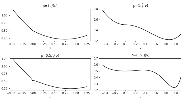
For $p=1$, the first row of fig. 2 shows the objective functions of $l_{p}$ eq. 32 and the transformed $l_{2}$ eq. 33 formulations. Each objective function has a unique global minimum without other local minima. The minimizers are $\frac{3}{4}$ and $\frac{\sqrt{3}}{2}$ for $l_{1}$ and $l_{2}$, respectively. We can check that the transformation does not add/remove local minimizers, but the convexity of the objective function changes. The transformed objective function $\tilde{J}$ has an inflection point at $u=0$, which is also a stationary point. Note that the original function has no other stationary points than the global minimizer.

When $p=0.5$, a potential issue of the transformation can be seen explicitly. The original objective and the transformed objective functions are shown in the second row of fig. 2. Due to the regularization term with $p=0.5$, the objective functions are non-convex and have a local minimizer at $u=v=0$ in addition to the global minimizers. In the transformed formulation (bottom right of fig. 2), the objective function flattens around $v=0$, which shows a potential issue of trapping ensemble members around $v=0$. Numerical experiments show that if the ensemble is initialized with a small variance, the ensemble is trapped around $v=0$. On the other hand, if the ensemble is initialized with a sufficiently large variance (so that some of the ensemble members are initialized out of the well around $v=0$), $l_{p}$EKI shows convergence to the true minimizer, $v=0.9304$ (or $u=0.8656$) even when it is initialized around $0$.

We use 100 different realizations for the ensemble initialization and each trial uses 50 ensemble members. The estimates at each iteration, which is averaged over different trials, are shown in fig. 3. For $p=1$ (first row) and $p=0.5$ (second row), the left and right columns show the results when the ensemble is initialized with mean 1 and 0, respectively. When $p=1$ and initialized around $1$, the ensemble estimate quickly converges to the true value $0.75$ as the objective function is convex, and the initial guess is close to the true value. When $p=0.5$, as the objective function is non-convex due to the regularization term, the convergence is slower than the $p=1$ case. When the ensemble is initialized around 0 for $p=0.5$, a local minimizer, the ensemble needs to be initialized with a large variance. Using variance 1, which is 10 times larger than 0.1, the variance for the ensemble initialization around 1, $l_{p}$EKI converges to the true value. The performance difference between different trials is marginal. The standard deviations of the estimate after 50 iterations are $6.62\times 10^{-3}$ ($p=1$ initialized with 1), $7.95\times 10^{-3}$ ($p=1$ initialized with 0), $8.79\times 10^{-3}$ ($p=0.5$ initialized with 1), and $1.14\times 10^{-2}$ ($p=0.5$ initialized with 0). As a reference, the estimate using the transformation eq. 22 based on matching the densities of random variables converges to 0.71.

The second test is a compressive sensing problem. The true signal $u$ is a vector in $\mathbb{R}^{200}$, which is sparse with only four randomly selected non-zero components (their magnitudes are also randomly chosen from the standard normal distribution.) The forward model $G:\mathbb{R}^{200}\to\mathbb{R}^{20}$ is a random Gaussian matrix of size $20\times 200$, which yields a measurement vector in $\mathbb{R}^{20}$. The measurement $y$ is obtained by applying the forward model to the true signal $u$ polluted by Gaussian noise with mean zero and variance $0.01$. As the forward model is linear, several robust methods can solve the sparse recovery problem, including the $l_{1}$ convex minimization method [4]. This test aims to compare the performance of $l_{p}$EKI for various $p$ values, rather than to advocate the use of $l_{p}$EKI over other standard methods. As the forward model is linear and cheap to calculate, the standard methods are preferred over $l_{p}$EKI for this test.

We first use a large ensemble size, 2000 ensemble members, to run $l_{p}$EKI. The ensemble is initialized by drawing samples from a Gaussian distribution with mean zero and a diagonal covariance (which yields variance 0.1 for each component). For $p=1$ and $0.7$, the tuned regularization coefficients, $\lambda$, are 100 and 300. When $p=2$, which corresponds to TEKI, the best result can be obtained using $\lambda$ ranging from 10 to 200; we use the result of $\lambda=50$ to compare with the other cases. For $p=1$, we also compare the result of the convex $l_{1}$ minimization method using the KKT solver in the Python library CVXOPT [20].

Figure 4 shows the $l_{p}$EKI estimates after 20 iterations averaged over 100 trials for $p=2$ (top left), $p=1$ (top right), and $p=0.7$ (bottom left), along with the estimate by the convex optimization (bottom right). As it is well known in compressive sensing, $l_{2}$ regularization fails to capture the true signal’s sparse structure. As $p$ decreases to 1, $l_{p}$EKI develops sparsity in the estimate, comparable to the estimate of the convex $l_{1}$ minimization method. The slightly weak magnitudes of the three most significant components by $l_{p}$EKI improve as $p$ decreases to $0.7$. When $p=0.7$, $l_{p}$EKI captures the correct magnitudes at the cost of losing the smallest magnitude component. We note that the smallest magnitude component is difficult to capture; the magnitude is comparable to the measurement error $0.1=\sqrt{0.01}$.

Another cost of using $p<1$ to impose stronger sparsity than $p=1$ is a slow convergence rate of$l_{p}$EKI. The time series of the $l_{1}$ estimation error and the data misfit of $l_{p}$EKI averaged over 100 trials are shown in fig. 5 alongside those of the convex optimization method. The results show that $p=0.7$ converges slower than $p=1$ (see Table table 1 for the numerical values of the error and the misfit). Although there is a slowdown in convergence, it is worth noting that $l_{p}$EKI with $p=0.7$ converges in a reasonably short time, 15 iterations, to achieve the best result. $l_{p}$EKI with $p=2$ converges fast with the smallest data misfit. However, the $l_{2}$ regularization is not strong enough to impose sparsity in the estimate and yields the largest estimation error, which is 20 times larger than the case of $p=1$. Note that the convex optimization method has the fastest convergence rate; it converges within three iterations and captures the four nonzero components with slightly smaller magnitudes than $p=0.7$ for the three most significant components.

The ensemble size 2000 is larger than the dimension of the unknown vector $u$, 200. A large ensemble size can be impractical for a high-dimensional unknown vector. To see the applicability of $l_{p}$EKI using a small ensemble size, we use 50 ensemble members and two batches following the multiple batch approach [23]. The first batch runs 10 iterations, and all components whose magnitudes are less than 0.1 (the square root of the observation variance) are removed. The problem’s size the second batch solves ranges from 30-45 (depending on a realization of the initial ensemble), which is then solved for another 10 iterations. The estimates using 50 ensemble members for $p=1$ and $p=0.7$ after two batch runs (i.e., 20 iterations) are shown in fig. 6. Compared with the large ensemble size case, the small ensemble size run also captures the most significant components at the cost of fluctuating components larger than the large ensemble size test. We note that the estimates are averaged over 100 trials, and thus there are components whose magnitudes are less than the threshold value 0.1 used in the multiple batch run.

As a measure to check the performance difference for different trials, fig. 7 shows the standard deviations of $l_{p}$EKI estimates for $p=1$ and $0.7$ after 20 iterations. The first row shows the results using 2000 ensemble members, while the second row shows the ones using 50 ensemble members. The standard deviations of the large ensemble size are smaller than those of the small ensemble size case as the large ensemble size has a smaller sampling error. In all cases, the standard deviations are smaller than 6% of the magnitude of the most significant components. In terms of $p$, the standard deviations of $p=0.7$ are smaller than those of $p=1$.

Next, we consider an inverse problem where the forward model is given by an elliptic partial differential equation. The model is related to subsurface flow described by Darcy flow in the two-dimensional unit square $(0,1)^{2}\subset\mathbb{R}^{2}$

$$-\nabla\cdot(k(x)\nabla p(x))=f(x),\quad x=(x_{1},x_{2})\in(0,1)^{2}.$$

(34)

The scalar field $k(x)>\alpha>0$ is the permeability, and another field $p(x)$ is the piezometric head or the pressure field of the flow. For a known source term $f(x)$, the inverse problem estimates the permeability from measurements of the pressure field $p$. This model is a standard model for an inverse problem in oil reservoir simulations and has been actively used to measure EKI’s performance and its variants, including TEKI [16, 8].

We follow the same setting used in TEKI [8] for the boundary conditions and the source term. The boundary conditions consist of Dirichlet and Neumann boundary conditions

$$p(x_{1},0)=100,\frac{\partial p}{\partial x_{1}}(1,x_{2})=0,-k\frac{\partial p}{\partial x_{1}}(0,x_{2})=500,\frac{\partial p}{\partial x_{2}}(x_{1},1)=0,$$

and the source term is piecewise constant

$$\displaystyle f(x_{1},x_{2})=\left\{\begin{array}[]{ll}0&\mbox{if }0\leq x_{2}\leq\frac{4}{6},\\ 137&\mbox{if }\frac{4}{6}<x_{2}\leq\frac{5}{6},\\ 274&\mbox{if }\frac{5}{6}<x_{2}\leq 1.\end{array}\right.$$

A physical motivation of the above configuration can be found in [7]. We use $15\times 15$ regularly spaced points in $(0,1)^{2}$ to measure the pressure field with a small measurement error variance $10^{{-6}}$. For a given $k$, the forward model is solved by a FEM method using the second-order polynomial basis on a $60\times 60$ uniform mesh.

In addition to the standard setup, we impose a sparse structure in the permeability. We assume that the log permeability, $\log k$, can be represented by 400 components in the cosine basis $\phi_{ij}=\cos(i\pi x_{1})\cos(j\pi x_{2}),i,j=0,1,...,19,$

$$\log k(x)=\sum_{i,j=0}^{19}u_{ij}\phi_{ij}(x),$$

(35)

where only six of $\{u_{ij}\}$ are nonzero. That is, we assume that the discrete cosine transform of $\log k$ is sparse with only 6 nonzero components out of 400 components. Thus, the problem we consider here can be formulated as an inverse problem to recover $u=\{u_{ij}\}\in\mathbb{R}^{400}$ (which has only six nonzero components) from a measurement $y\in\mathbb{R}^{225}$, the measurement of $p$ at $15\times 15$ regularly spaced points. In terms of sparsity reconstruction, the current setup is similar to the previous compressive sensing problem, but the main difference lies in the forward model. In this test, the forward model is nonlinear and computationally expensive to solve, where the forward model in the compressive sensing test was linear using a random measurement matrix.

For this test, we run $l_{p}$EKI using only a small ensemble size due to the high computational cost of running the forward model. As in the previous test, we use the multiple batch approach. First, the $l_{p}$EKI ensemble of size 50 is initialized around zero with Gaussian perturbations of variance 0.1. After the first five iterations, all components whose magnitudes less than $5\times 10^{-3}$ are removed at each iteration. The threshold value is slightly smaller than the smallest magnitude component of the true signal. Over 100 different trials, the average number of nonzero components after 30 iterations is 18 that is smaller than the ensemble size.

The true value of $u$ used in this test and its corresponding log permeability, $\log k$, are shown in the first row of fig. 8 ($u$ is represented as a one-dimensional vector by concatenating the row vectors of $\{u_{ij}\}$). The $l_{p}$EKI estimates for $p=2,1$, and $0.8$ are shown in the second to the fourth rows of fig. 8. Here $p=0.8$ was the smallest value we can use for $l_{p}$EKI due to the numerical overflow in the exponentiation of $\log k$. A smaller $p$ can be used with a smaller variance for ensemble initialization, but the gain is marginal. The results of $l_{p}$EKI are similar to the compressive sensing case. $p=0.8$ has the best performance recovering the four most significant components of $u$. $p=1$ has slightly weak magnitudes missing the correct magnitudes of the two most significant components (corresponding to one-dimensional indices 141 and 364). Both cases converge within 20 iterations to yield the best result (see fig. 9 and Table table 2 for the time series and numerical values of the $l_{1}$ error and data misfit). When $p=2$, $l_{p}$EKI performs the worst; it has the largest $l_{1}$ error and data misfit. We note that $p=2$ uses the result after running 50 iterations at which the estimate converges.

The performance difference between different trials is not significant. The standard deviations of the $l_{p}$EKI estimates using 100 trials are shown in fig. 10. The standard deviations for nonzero components are larger than the other components, but the largest standard deviation is less than 3% of the magnitude of the true signal. As in the compressive sensing test, the deviations are slightly smaller for $p<1$ than $p=1$.

References

- [1] J. L. Anderson, An ensemble adjustment kalman filter for data assimilation, Monthly Weather Review, 129 (2001), pp. 2884–2903.
- [2] J. M. Bardsley, A. Solonen, H. Haario, and M. Laine, Randomize-then-optimize: A method for sampling from posterior distributions in nonlinear inverse problems, SIAM Journal on Scientific Computing, 36 (2014), pp. A1895–A1910.
- [3] M. Benning and M. Burger, Modern regularization methods for inverse problems, Acta Numerica, 27 (2018), p. 1–111.
- [4] S. Boyd and L. Vandenberghe, Convex Optimization, Cambridge University Press, USA, 2004.
- [5] A. C. Reynolds, M. Zafari, and G. Li, Iterative forms of the ensemble kalman filter, (2006).
- [6] E. J. Candès, M. B. Wakin, and S. P. Boyd, Enhancing sparsity by reweighted minimization, Journal of Fourier Analysis and Applications, 14 (2008), pp. 877–905.
- [7] J. Carrera and S. P. Neuman, Estimation of aquifer parameters under transient and steady state conditions: 3. application to synthetic and field data, Water Resources Research, 22 (1986), pp. 228–242.
- [8] N. K. Chada, A. M. Stuart, and X. T. Tong, Tikhonov regularization within ensemble kalman inversion, SIAM Journal on Numerical Analysis, 58 (2020), pp. 1263–1294.
- [9] N. K. Chada and X. T. Tong, Convergence acceleration of ensemble kalman inversion in nonlinear settings, (2019). arXiv:1911.02424.
- [10] J. Duchi, E. Hazan, and Y. Singer, Adaptive subgradient methods for online learning and stochastic optimization, J. Mach. Learn. Res., 12 (2011), p. 2121–2159.
- [11] G. Evensen, Data Assimilation: The Ensemble Kalman Filter, Springer, London, 2009.
- [12] R. Fletcher, Practical methods of optimization, John Wiley, New York, 2nd ed., 1987.
- [13] S. Foucart and H. Rauhut, A Mathematical Introduction to Compressive Sensing, Birkhäuser Basel, 2013.
- [14] I. Goodfellow, Y. Bengio, and A. Courville, Deep Learning, The MIT Press, 2016.
- [15] M. Hanke, A regularizing levenberg - marquardt scheme, with applications to inverse groundwater filtration problems, Inverse Problems, 13 (1997), pp. 79–95.
- [16] M. Iglesias, K. J. H. Law, and A. Stuart, Ensemble kalman methods for inverse problems, Inverse Problems, 29 (2013), p. 045001.
- [17] M. A. Iglesias, A regularizing iterative ensemble kalman method for PDE-constrained inverse problems, Inverse Problems, 32 (2016), p. 025002.
- [18] N. B. Kovachki and A. M. Stuart, Ensemble kalman inversion: a derivative-free technique for machine learning tasks, Inverse Problems, 35 (2019), p. 095005.
- [19] A. C. Li, Gaoming; Reynolds, An iterative ensemble kalman filter for data assimilation, (2007).
- [20] L. V. M.S. Andersen, J. Dahl, Cvxopt: A python package for convex optimization. cvxopt.org.
- [21] D. Oliver, A. C. Reynolds, and N. Liu, Inverse Theory for Petroleum Reservoir Characterization and History Matching, Cambridge University Press, Cambridge, UK, 1st ed., 2008.
- [22] B. T. Polyak and A. B. Juditsky, Acceleration of stochastic approximation by averaging, SIAM Journal on Control and Optimization, 30 (1992), pp. 838–855.
- [23] H. Schaeffer, Learning partial differential equations via data discovery and sparse optimization, Proceedings of the Royal Society A: Mathematical, Physical and Engineering Sciences, 473 (2017), p. 20160446.
- [24] C. Schillings and A. M. Stuart, Analysis of the ensemble kalman filter for inverse problems, SIAM Journal on Numerical Analysis, 55 (2017), pp. 1264–1290.
- [25] T. Schneider, A. M. Stuart, and J.-L. Wu, Imposing sparsity within ensemble kalman inversion, (2020). arXiv:2007.06175.
- [26] Z. Wang, J. M. Bardsley, A. Solonen, T. Cui, and Y. M. Marzouk, Bayesian inverse problems with $l_1$ priors: A randomize-then-optimize approach, SIAM Journal on Scientific Computing, 39 (2017), pp. S140–S166.