Low-energy peak in the one-particle spectral function of the electron gas
at metallic densities
Abstract
Based on a nonperturbative scheme to determine the self-energy with automatically satisfying the Ward identity and the total-momentum conservation law, a fully self-consistent calculation is done in the electron gas at various temperatures to obtain the one-particle Green’s function with fulfilling all known conservation laws, sum rules, and correct asymptotic behaviors; here, is taken unprecedentedly low, namely, down to with the Fermi energy, and tiny mesh as small as is chosen near the Fermi surface in space with the Fermi momentum. By analytically continuing to the retarded function , we find a novel low-energy peak, in addition to the quasiparticle (QP) peak and one- and two-plasmon high-energy satellites, in the spectral function for in the simple-metal density region ( with the dimensionless density parameter). This new peak is attributed to the effect of excitonic attraction on arising from multiple excitations of tightly-bound electron-hole pairs in the polarization function for and and thus it is dubbed “excitron”. Although this excitron peak height is only about a one-hundredth of that of QP, its excitation energy is about a half of that of QP for , seemingly in contradiction to the Landau’s hypothesis as to the one-to-one correspondence of low-energy excitations between a free Fermi gas and an interacting normal Fermi liquid. As for the QP properties, our results of both the effective mass and the renormalization factor are in good agreement with those provided by recent quantum Monte Carlo simulations and available experiments.
I Introduction
The Landau Fermi-liquid theory (FLT) [1, 2] is very useful in describing low-temperature physics in ordinary metals through the concept of quasiparticle (QP). This key concept is verified to infinite order in perturbation expansion in the quantum field theory [3, 4, 5, 6]. It is also confirmed in both the renormalization-group approach [7] and the multidimensional bosonization [8, 9, 10].
In these several decades, FLT is found to break down in a number of exotic metals broadly referred to as non-Fermi liquids (NFLs), including the one-dimensional (1D) Luttinger liquids [11, 12, 13, 14, 15], the strange-metal phase in high- cuprates [16, 17, 18, 19, 20, 21], and the fluctuation regime around a quantum critical point (QCP) [22, 23, 24, 25, 26, 27, 28, 29, 30, 31, 32, 33, 34, 35].
It has been quite a challenge to fully understand the routes to NFLs from normal Fermi liquids [36, 37, 38, 39, 40, 41, 42]. In 3D simple metals, we can envisage a couple of routes to NFLs. The first one is related to the long-range nature of the Coulomb interaction (). In fact, this has been investigated in detail in the past [43, 44, 45] and it is concluded that at is not singular enough to break FLT in 3D metals due to the screening effect. Incidentally, transverse electromagnetic fields give rise to unscreened long-range interactions, leading to the breakdown of FLT even in alkali metals [46, 47, 48], but this occurs only at unrealistically low temperatures because of its very weak coupling controlled by the small factor , where is the Fermi momentum, is the mass of a free electron, and is the velocity of light. Hereafter we employ units in which .
The second route is concerned with the response function at and possible singularities in it [49, 50, 9, 51, 45, 10, 52, 26, 53]. This is a problem which has not been examined in detail, especially in the context of 3D simple metals. The density response at low energies and short wavelengths will be an essential ingredient in the present study, as we now explain.
The low-lying excited states in simple metals are well described by those of a 3D homogeneous electron gas, an assembly of electrons embedded in a uniform positive rigid background. In a recent paper [54], it is shown in the low-density electron gas that an excitonic collective mode made of correlated electron-hole pair excitations appears as a soft mode for . If this vanishes at , then a macroscopic number of electron-hole pairs are produced spontaneously to form a CDW state with the wave number which is exactly the state predicted by Overhauser [55]. In actual simple metals for which the density parameter defined by
| (1) |
and the Bohr radius is in the range from 2 to 6, this kind of CDW does not seem to exist, but from the perspective of QCP physics, the correlated electron-hole pair excitations around may be regarded as quantum fluctuations around the quantum critical CDW transition point. In this regard, those bosonic excitations in simple metals can be considered as marginally relevant processes in the sense of renormalization group to break FLT.
In fact, the above-mentioned mode is confirmed as an incipient excitonic mode in the dynamic structure factor at by recent ab initio path integral Monte Carlo simulations performed in the electron gas for - [56, 57, 58] and - [59], where the mode is referred to as a “roton”.
In this paper, by exploiting the precise polarization function in the charge channel derived from Monte Carlo data for the density response, we will accurately calculate the self-energy with , a combined notation of momentum and fermion Matsubara frequency , in the 3D homogeneous electron gas for with the motivation to inspect the validity of FLT in simple metals. For this inspection, we are not allowed to adopt a theory based on any kinds of perturbation expansion, because NFL cannot be described by perturbation expansion starting from the noninteracting Green’s function ; actually, the so-called approximation to the Hedin’s closed set of equations, derived by using the screened interaction as an expansion parameter [60, 61, 62, 63, 64, 65], and its refinements [66, 67, 68, 69] have not shown any indication of the breakdown of FLT. The same is true both in the many-body perturbation theory with using some appropriate local-field factor [70, 71, 72, 73, 74, 75, 76] and in the effective-potential expansion (EPX) method [77, 78].
Considering this situation, we shall employ the GW scheme [79] which is improved on the original one [80] and satisfies all the known conservation laws and sum rules, including the Ward identity (WI) [81], total-energy and total-momentum conservation laws, three sum rules concerning the momentum distribution function [54], and correct asymptotics. This scheme is an intrinsically nonperturbative approach applicable to both Fermi and Luttinger liquids in a unified manner [82], but so far, it was too complicated to be implemented in 3D systems. In particular, the total-momentum conservation law (and thus the backflow effect) was not well respected, so that the QP effective mass could not be reliably determined. Therefore, one of the aims in this paper is to develop a feasible code to implement this advanced scheme with keeping the total-momentum conservation law.
By applying this newly developed code to the electron gas at , , , , , and relevant to Al, Li, Na, K, Rb, and Cs, respectively, we successfully obtain a convergent result of at each and various values of down to , where is the Fermi energy. For , the obtained is not smooth enough at and to safely confirm FLT; by a heuristic analysis, this anomalous behavior is found to be well described by a branch-cut singularity, exhibiting a symptom of possible breakdown of FLT.

This situation is more clearly seen in the one-particle spectral function with and the retarded Green’s function obtained by an analytic continuation of in complex plane through Padè approximants. A typical example of , a quantity to be observed by angle-resolved photoemission spectroscopy (ARPES), is shown in Fig. 1 in which a new peak indicated by “excitron” appears in addition to the predominant QP peak and one- and two-plasmon satellites. It is evident from this figure that an energy resolution in ARPES should be of the order of 1 meV or less to experimentally distinguish this weak excitron peak from the very strong QP peak.
Since the excitron spectral strength is quite weak and is dominated by the QP pole singularity, bulk properties of the electron gas at metallic densities will be well explained by FLT in which the quantitative evaluation of is a long-standing yet hot issue. We can determine from the QP peak position at in the vicinity of ; our values for are in good agreement with those given in recent quantum Monte Carlo (QMC) simulations [83, 84]. The same is true for the QP renormalization factor ; our values for determined by the jump of at agree well with those in recent QMC simulations [85, 86] and available experiments [86, 87, 88].
This paper is organized as follows: In Sec. II we explain our framework to calculate in the electron gas through a nonperturbative iteration loop with rigorously satisfying the Ward identity and the total-momentum conservation law. A proposed functional form for the vertex function in Sec. II.5 is one of our main results. In Sec. III we give the calculated results on various properties in the electron gas, including a new low-energy peak dubbed excitron and two-plasmon satellites in . Although we treat the electron densities corresponding to all simple metals, the main stress is laid on Na, because Na is known to be an almost perfect realization of the electron gas with . In Sec. IV we make a detailed account of the excitron, ascribing it to the effect of excitonic attraction arising from multiple excitations of tightly bound electron-hole pairs. Finally in Sec. V we give a summary of this paper and discuss related and future issues. Appendices AE provide some details of our numerical calculation.
II Self-Energy Calculation Scheme
II.1 Hamiltonian
The Hamiltonian for a 3D homogeneous electron gas is written in second quantization as
| (2) |
where is the annihilation operator of an electron with momentum and spin whose single-particle energy is given by with . We will consider the system in unit volume and the total number of electrons is nothing but the electron density , given in terms of the Fermi momentum as .
In this system, the correlation energy per electron is already known accurately as a function of by the Green’s-Function Monte Carlo (GFMC) method [89] and the interpolation formulas to reproduce the GFMC data [90, 91]. With the use of , the correlation contribution to the chemical potential and the compressibility are, respectively, obtained as
| (3) | ||||
| (4) |
where is given through the thermodynamic relation of and is the compressibility in the noninteracting electron gas, given by with the density of states at the Fermi level in the noninteracting system.
II.2 One-particle Green’s function
The Dyson equation relates the one-particle Green’s function with the self-energy through
| (5) |
Here, is divided into with the exchange contribution to , given by
| (6) |
Let us divide into odd and even parts in as
| (7) |
where both and are not only even functions in but also real functions, as seen by combining Eq. (7) with the analyticity property . Then, is rewritten as
| (8) |
with the introduction of .
II.3 Momentum distribution function
Once is known, the momentum distribution function is calculated as
| (9) |
where the Matsubara sum is taken by the procedure explained in Appendix A. Accuracy of may be checked by the three sum rules related to total electron number, total kinetic energy, and total kinetic-energy fluctuation, as derived in Ref. [54]. Those sum rules are conveniently expressed in terms of the th-power integral , given as
| (10) |
with and . The rigorous values for with , , and are: , , and with the on-top value of the pair distribution function and specified in Eq. (51) in Ref. [54]. After several tentative calculations, we find that as obtained from Eq. (9) satisfies the sum rule up to five digits or more and up to three digits, but up to only a single digit in most cases, indicating that for is not accurate enough, which reflects the fact that the -mesh (or grid) in space in the iterative calculation of is not dense enough for .
As a remedy for this problem in , we have modified to by the procedure explained in Appendix B in which the behavior in the region of is rectified by the introduction of obtained by the parametrization scheme described in Ref. [54]. In actual calculations, always satisfies all the three sum rules up to at least five digits (and mostly seven or eight digits). As an example, the results of , , and are shown for in Fig. 10(a) in which we can barely see the difference among those three functions on the scale of the figure.
II.4 Polarization function
The charge response function is related to the polarization function in the charge channel through
| (11) |
and the formal definition of is written as
| (12) |
where is the three-point vertex function in the charge channel.
In the many-body problem, it is often the case that is less singular than . In fact, in 1D Luttinger liquids, is easily obtained and does not exhibit any NFL-related singularity [12]. In 3D Fermi liquids, it is shown that no nonanalytic corrections are contained in , in sharp contrast to the polarization function in the spin channel in which a nonanalytic -term exists [52]. Thus we can expect that in the 3D electron gas, even if there were a branch-cut singularity in at low , it would not induce any singular effects on , implying that will be reliably determined even at of the order of . On this assumption, we consider obtained by Monte Carlo simulations [92, 93, 97, 94, 95, 98, 96] as sufficiently accurate data, based on which various parametrized forms for the conventional charge local-field factor have been proposed [99, 100, 101, 102, 103, 104, 105].
In view of this situation, we regard as a quantity precisely known from the outset in the self-consistent iteration loop. In actual calculations, is given either with as
| (13) |
or with due to Richardson and Ashcroft [99] as
| (14) |
where the Lindhard function is calculated as [106]
| (15) |
with the step function and is given by
| (16) |
Note that is obtained from as
| (17) |
but in this paper, we shall adopt the function form (a slightly modified Richardson-Ashcroft parametrization) prescribed in Eq. (58) in Ref. [54] for .
In Eq. (16), we employ for to make correctly behave in the limit of . On the other hand, the behaviors of and in the limit of can be derived directly from Eqs. (II.4) and (16), respectively; in the -limit (i.e., first, and then ), we obtain
| (18) |
with and in the -limit (i.e., first, and then ), we obtain
| (19) |
where is defined in Eq. (10) with . Combining the above-mentioned behavior of with the constraints imposed on (or that of with those on ) at , we see that in the -limit,
| (20) |
and in the -limit,
| (21) |
The relations in Eqs. (20) and (21) are, respectively, known as the f-sum rule and the compressibility sum rule.
II.5 Vertex function
Formally, we can calculate rigorously by
| (22) |
where is the effective interaction, given by
| (23) |
Since we regard as a precisely known quantity, is already known. As for , we adopt the improved scheme described in Ref. [79]. According to Eqs. (54)-(58) in Ref. [79], is given in the product of two components as
| (24) |
with
| (25a) | |||
| (25b) | |||
where the functional is introduced as
| (26) |
and three “modified polarization functionals”, , , and , are, respectively, defined as
| (27a) | ||||
| (27b) | ||||
| (27c) | ||||
The functional will be specified later.
In Ref. [79], this functional form for was derived from the perspective of FLT, i.e., with the assumption that is given in such a form as
| (28) |
for and , where , , and are, respectively, the QP renormalization factor, the QP dispersion, and the QP lifetime. Here, is assumed and is a smooth function, corresponding to the incoherent smooth background in . Note that QP appears as a pole in as long as and this pole-singularity is intimately connected with the condition that is smooth enough to be analytically expanded around the Fermi point .
The final result in Eq. (24), together with Eqs. (25)-(27), however, does not explicitly contain any FLT-specific parameters such as the Landau interaction and , implying that this functional form itself can be applied to NFL as well. In fact, , a key quantity leading to at in FLT, appears in this formalism as a direct consequence of the total-current (or total-momentum) conservation law that should be satisfied even in NFL, indicating that must also be a key quantity in NFL.
It is the most important advantage in this formalism that the Ward identity (WI) [81] is automatically satisfied, whatever choice one may make for and ; if we choose , the present vertex function is nothing but the one in the original scheme [80] and is reduced to the canonical form appearing in connection to WI as
| (29) |
Thus, we note that by just changing into , we can enter into a more advanced stage in which both WI and the total-momentum conservation law are simultaneously fulfilled.
In actual numerical calculations, however, it turns out that it is not easy to proceed at each iteration step with evaluated in accordance with Eq. (26). Because reflects the total-momentum conservation law only in its value at , we can approximate as , a function depending only on with the condition that in the -limit. Under this approximation, we can reduce into
| (30) |
and is easily calculated by
| (31) |
with in Eq. (16).
Since we may take at our disposal, we choose it so as to make numerical calculations as easy as possible. By carefully inspecting the structure of each term in Eq. (30), we can think of a possible form for as
| (32) |
with arbitrary functions (, and ). By substituting this into Eq. (30), we immediately find the following: (i) is irrelevant, because it is always cancelled by the corresponding term in . (ii) By choosing as , we can eliminate the first term in the curly brackets in Eq. (30). (iii) Because the term containing is rather difficult to treat, it would be better to approximate by with . As a result, we have arrived at the functional form for , written as
| (33) |
It should be noted that we can rigorously reproduce irrespective of and in substituting this functional form for into Eq. (II.4), verifying the internal consistency of our formulation.
To determine and , we need to consider several constraints to be imposed on them to make behave correctly in various limits. In line with such constraints as discussed in Appendix C, we will use in Eq. (C3) and given by
| (34) |
in this paper.

In Fig. 2, the self-consistently determined results of are plotted at for the 3D homogeneous electron gas with . As seen from this figure, is smoothly converged to unity for , but it exhibits a rather rapid change near , indicating that is not smooth enough for , a symptom of possible breakdown of FLT. Incidentally, in obtaining , we need to know the static physical quantities, and , which can be obtained by an extrapolation procedure explained in Appendix D.

In Eq. (34), the term involving the parameter is introduced to rigorously reproduce , the value accurately given in Eq. (3). The appropriately determined values for providing the correct with in the region of are shown in Fig. 3 in which we take as . As seen from the figure, the magnitude of is small, i.e., of the order of 0.02, letting us know that the term exerts only limited effects on .
II.6 Self-energy
By substituting Eq. (33) with Eq. (34) into Eq. (22), we obtain an expression for the calculation of as
| (35) |
with
| (36a) | |||
| (36b) | |||
| (36c) | |||
where , , , and are, respectively, defined as
| (37a) | |||
| (37b) | |||
| (37c) | |||
| (37d) | |||
Here, is independent of and directly connected to the chemical potential shift, is the main contribution to the self-energy, and partially contributes to the renormalization factor.
II.7 Self-consistent iteration loop
To summarize this section, Fig. 4 schematically displays a self-consistent iteration loop to determine . In developing the actual code, we make it adaptable to calculations at unprecedentedly low temperatures, down to , because no singularities in leading to NFL have been obtained for in the original GW scheme [80], in the recent variational diagrammatic Monte Carlo (VDMC) simulations [97, 83], and in the algorithmic Matsubara-diagrammatic Monte Carlo (ADMC) technique [98]. In accordance with , the mesh size in space should also be small of the same order, i.e., near the Fermi surface, to detect any singularities in appearing at such a low , because at is approximately equal to which must be comparable to . In this respect, no symptoms of NFL will be detected in the recent zero-temperature quantum Monte Carlo calculations [84] in which is not small enough.

The implementation of this iteration loop starts with the self-energy in the random-phase approximation (RPA) (or the approximation [107]), given by
| (38) |
and ends up when the relative difference in between input and output at each mesh point becomes less than . In revising the input at each step during the iteration loop, we employ the second Broyden’s method [108, 109, 110]. We need - iteration steps depending on and to obtain converged results for . The calculated is converted into the retarded self-energy with through numerical analytic continuation with the use of Padé approximants [111].
In the actual numerical implementation, instead of , we calculate a couple of real functions in Eq. (8), and , both of which are even in and depend on only through . Those functions will be evaluated only at a finite number of points in -space, , and if we need the values of those functions at other than those selected points, then we will employ the two-dimensional cubic spline interpolation method. In Appendix E, we make a more detailed explanation of , together with some remarks on the numerical integration in Eqs (36a)-(36c) and the numerical analytic continuation.
III Calculated Results
III.1 One-particle spectral function

In Fig. 5, the one-particle spectral function is plotted as a function of for , corresponding to sodium, at with in units of . This shows a well-known typical behavior, characterized by the dominant quasiparticle peak and the associated one-plasmon satellites. In fact, this result is essentially the same, even quantitatively, as the one given at in Fig. 3(a) in Ref. [79] in which both and were taken as unity. Therefore, we cannot find any indication of the breakdown of FLT at least for sodium at , as is the case in all previous studies on alkali metals.
By decreasing down to , however, we find a totally new situation in the low-energy region of for at , as shown in Fig. 6. Although nothing special is seen at at all temperatures, a shoulder or bump structure begins to develop at and a clear peak structure emerges at for not equal to but close to it. The energy of this new peak is about a half of that of the corresponding quasiparticle peak at the same and thus a new mode, if any, associated with this peak (to be dubbed “excitron”) is characterized by the very low excitation energy of the order of or less.

In Fig. 7, we show the change in shape and position of this new peak with the increase of from to through for at , from which we see that this new peak is absorbed into (or perfectly overlapped with) the dominant quasiparticle peak at . Thus, we need to keep away from to detect this new peak, but at the same time, as increases, the peak height decreases, making the detection rather difficult. To compromise between these competing factors, it would be good to search for this peak at in the range . We have also calculated at for other values of in the range of to find that this new peak always appears with qualitatively the same features as those described above, including the behavior with the change of and , though quantitatively the peak strength (or height) depends rather strongly on ; as increases, the peak emerges more vividly and strongly. A more detailed analysis on the character of this new peak (or excitron) will be made in Sec. IV.

The dispersion relation of excitron (or the peak position of this new mode), , at for and corresponding to Na and Rb, respectively, is drawn in Fig. 8, together with the quasiparticle dispersion relation determined by the quasiparticle peak position and the bare dispersion . Although the results for corresponding to K are not shown here, they enter just between those of Na and Rb. For , is not shown, because the new peak in either or becomes broad and its peak height is very low, making us very difficult to identify the peak position or the peak itself. For , the excitron dispersion is linear and can be written as , but for not in the vicinity of , deviates from this linear relation. The ratio of is plotted as a function of in Fig. 12 in Sec. III.4.

The quasiparticle effective mass estimated by with in the range of is about the same as , but it becomes smaller than for outside of this range. This change of with can easily be understood by the fact that is determined by the competition of exchange and correlation effects; the former makes small as understood by the fact that at in the exchange-only (or Hartree-Fock) approximation, while the latter makes large as easily guessed by just considering the heavy-fermion physics. Because the exchange effect is evaluated in first-order perturbation theory (and thus without energy denominators), it persists even for far away from . This is not the case for the correlation effect to which the second- and higher-order perturbation terms contribute. Thus, as goes away from the Fermi level, the correlation effect becomes weaker than that of exchange, making smaller than . In this way, the dispersion relation can never be parabolic in the whole region of from to , making the occupied bandwidth wider than that of the free-electron band. This widened bandwidth is also seen in the diffusion Monte Carlo (DMC) simulations [113, 112] as shown by the brown curve in Fig. 8; the magnitude of bandwidth in DMC is about the same as that in the present calculation, though its behavior of for is much different, providing much smaller than which is not correct as we shall see in Sec. III.4. Note that DMC was feared to be an unreliable method in determining [114].
In contrast to this widening of the computed occupied bandwidth, much narrower bandwidths have been observed by ARPES experiments [115, 116]. To account for this discrepancy, various explanations were proposed; in particular, the effect of final states in the optical measurements attracted attention [117, 80], but very recently yet another plausible explanation was proposed by emphasizing the importance of local dynamical correlations associated with an atom based on a more realistic model beyond the electron gas [118].

In Fig. 9, is plotted on the hundred times wider scale of for in the range of in units of at and . On this large (not logarithmic but linear) scale, the excitron peak is not seen well as a separate structure from the dominant quasiparticle peak even at this very low , but we can detect the structures associated with the energies of the order of instead. In fact, we can easily find the one-plasmon satellites (shown by blue smaller arrows) and also even the two-plasmon ones (shown by red larger arrows).
The two-plasmon satellite is a challenging issue in the theoretical studies of photoemission in the electron gas in connection with experiments in simple metals. In the usual and related schemes, it is known to be very difficult to provide this two-plasmon satellite structure, which urged Aryasetiawan et al. to invent a plus cumulant-expansion approach [119], a method manually including the multiplasmon satellites. Afterwards, many other works followed in that direction [120, 121, 122, 123, 124], whereas Pavlyukh et al. succeeded in obtaining the structure without resort to the cumulant expansion for the first time [125]. As seen in Figs. 1 and 9, our present method is the second one to accomplish the goal of obtaining the two-plasmon satellites without manually including the multiplasmon satellites, as far as the author knows. More details on this important achievement may be published elsewhere in the future, along with data for wider ranges of and comparisons with other related works.
III.2 Momentum distribution function
The momentum distribution function is calculated for in the range of at in accordance with the prescription described in Sec. II.3, together with Appendix B, in which three functions, defined in Eq. (9), , and , are introduced. As shown in Fig. 10(a), we cannot see the difference among those three functions at on the scale of this figure. In fact, as long as , those three functions provide virtually the same result. Even for , a small difference between and appears only for . Therefore, in Fig. 10(b), we give only the results of which satisfies all the three sum rules associated with , , and very accurately up to seven digits. We have also calculated at several other temperatures up to to find that the obtained results are virtually independent of . Incidentally, the present results of are essentially the same as those of the momentum distribution function given in Sec. II F in Ref. [54].

For comparison, the results of at in quantum Monte Carlo (QMC) simulations for the 3D homogeneous electron gas [85] (blue dotted-dashed curve) and the solid sodium [126] (green diamonds) are depicted in Fig. 10(a). The data in QMC are seen to be in reasonably good agreement with our present ones, but we do not regard the QMC data as sufficiently accurate ones for the following reasons: (i) The QMC data are not verified to satisfy the three sum rules. In fact, by just looking at the difference between in QMC and perfectly satisfying the three sum rules, we would consider that the QMC data might satisfy the sum rule, but they never satisfy other sum rules. (ii) The size extrapolation, an inevitable process in QMC to obtain physical quantities in the bulk system, is not reliable enough to produce a definite and well-converged result, as mentioned in Ref. [79]. (iii) If we compare the results given by the blue dotted-dashed curve with those by the green diamonds, the difference might be ascribed to the band effect. This effect, however, should not be large for , while the actual difference between them is unphysically large at , indicating that the magnitude of errors in the QMC evaluation is of the order of this size.
III.3 Quasiparticle renormalization factor
In all preceding works in which FLT was assumed to be valid, the quasiparticle renormalization factor is nothing but . In the present study, however, the quasiparticle peak is overlapped with that of excitron at as seen in Fig. 7, implying a possibility that differs from . Because we will come to know in Sec. IV that the singularity associated with the excitron is well described by a branch cut, we do not expect any contribution from the excitron to the jump of at the Fermi level, suggesting us to consider this jump as . At the same time, we may regard the difference between and the jump as the strength of the excitron peak at the Fermi level, , namely,
| (39) | ||||
| (40) |
In actual calculations, we find that defined in Eq. (40) is always positive, which is consistent with our interpretation of from a physical point of view.

In Fig. 11, we plot our results of and as a function of by green solid curve with circles and red solid curve with squares, respectively. For reference, the data for and are also given by the black dotted curves. This figure clearly shows that is larger than by times, implying that the excitron will exert its effect, if any, on bulk physical quantities by only a very small amount for .
For comparison, the preceding results of in both experiments and theories are added to the figure: Compton-scattering studies were done on Al [87], Li [127, 86], and Na [88] and the obtained results are indicated by the big black solid circles with error bars, while the data in QMC [85, 86] are by the big brown squares. For the sake of reference, the results of in and EPX methods are, respectively, shown by the blue dashed and purple dotted-dashed curves. We find that (i) our results of perfectly reproduce those experimental ones, (ii) they are also in very good agreement with the QMC data, and (iii) they are virtually the same as the old data in EPX, confirming the accuracy of the results in Ref. [128].
In the literature, it is often the case that the results of are given to be much higher than our present results or even those in , but those results are not correct, simply because such results originate from an inappropriate treatment of the correlation effect near the Fermi level where the energy denominators diverge. As discussed in rather details in Ref. [128], any theoretical frameworks without correctly taming the divergent energy denominators will fail to produce correct values of . To be more concrete, a theory with the use of Jastrow-type variational trial functions is, in general, not a good choice. Even in QMC or DMC, if those simulations start with Jastrow-based variational Monte Carlo, then final results may inherit the demerits of Jastrow functions. This might be one of the reasons why DMC does not provide correct near the Fermi level in Fig. 8.
III.4 Quasiparticle effective mass
The quasiparticle effective mass can be determined through the derivative of at and the obtained result is drawn by the green solid curve with circles in Fig. 12. Our present result is very close to that of Simion and Giuliani [74] given by the black dashed curve and it is also in excellent agreement with the very recent data provided by diagrammatic Monte Carlo calculation [83] (blue diamonds) and QMC [84] (brown squares). The result in shown by the black dotted curve is not quite the same as ours, but it may still be regarded as a semiquantitatively good result. This success of probably reflects the fact that itself is well reproduced by due to the strong mutual cancellation between the self-energy effect and the vertex correction as a consequence of the Ward identity [107]. Thus, if we are not concerned with the physics of highly correlated phenomena such as excitron, then is a good choice for many purposes, because it is computationally very cheap yet provides qualitatively correct results.

Compared with the quasiparticle velocity at the Fermi level , the velocity of excitron at the Fermi level , which can be obtained through the derivative of at , is found to be typically about a half of , as seen in Fig. 12 in which is shown in units of by the red solid curve with squares.
IV Details of Excitron
So far, the excitron is introduced only as a new low-energy peak in , but here we try to understand its features in terms of the self-energy, either the retarded one or the thermal one . For this purpose, we focus exclusively on the case of at in Secs. IV.1IV.4, partly because this is a typical example exhibiting a clear excitron peak in and partly because we can obtain a completely convergent result of much more easily in this system than in those at larger and/or lower . In Sec. IV.5, we examine the -dependence of by changing in the range of -.
IV.1 Characteristics of excitron in

In Fig. 13(a), in this system is drawn in a logarithmic scale as a function of at . For in the range , there exist four peaks in and the corresponding structure in is given in Fig. 13(b); at the quasiparticle peak position, both real and imaginary parts in vary very smoothly with vanishingly small magnitudes, as shown in the inset, in accordance with the assumption in FLT. On the other hand, the one-plasmon satellites are associated with large variations in both real and imaginary parts in the shape of functions as can be found in the Lorentz oscillator model, reflecting an electron motion in the electric field induced by the plasmon. At the excitron peak position, although the magnitudes of the variations are by far small, about a one-hundredth, the real and imaginary parts behave in a way very similar to those at the one-plasmon satellites, implying that the excitron peak must also be connected with the motion of an electron in the field induced by some kind of low-energy (of the order of ) excitations.
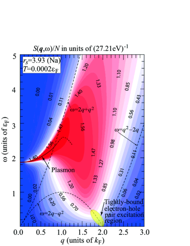
To pinpoint the relevant low-energy excitations to bring about the excitron, we show the calculated result of the structure factor , defined by
| (41) |
in Fig. 14 to demonstrate that, though the plasmon contribution in the range of with overwhelmingly dominates, the most important contribution in the range of comes from the tightly bound electron-hole pair excitations with , the region indicated by the yellow shaded area in the figure. Incidentally, the result for in Fig. 14 is virtually the same as that given for in Fig. 1(a) in Ref. [54], basically because the present result for is essentially the same as those in the previous publications, not only in Ref. [54] but also in Refs. [129, 130].
Now, our task is to study the electron-electron interaction mediated by the tightly bound electron-hole pair excitations and its contribution to the self-energy ; diagrammatically, they are given in Figs. 15(a) and 15(c), respectively, with the electron-hole irreducible (defined in the horizontal view) four-point interaction in Fig. 15(b). For and an electron on the Fermi sphere, i.e., , the dominant contribution to comes from the scattered states also on the Fermi sphere. Since , this is only possible for and . A similar restriction also applies to each pair polarization process in in Fig. 15(a); the important contribution arises only for in and in . The above restrictions clearly indicate that once we choose an electron characterized by , all the processes of its scatterings and the associated electron-hole pair excitations occur predominantly in either parallel or antiparallel to the -direction.


If we approximate and by and , respectively, in Fig. 15(a), then we can easily obtain an approximate expression for as
| (42) |
This is an attractive interaction and its importance was well appreciated long ago by the systematic and unbiased survey of the electron-electron interaction in the problem of superconductivity in the electron gas [131]. Because the relevant interaction is attractive, we can understand why the excitron energy is lower than .
IV.2 Extraction of the singular part in

After much trial and error, we come to realize that the mathematical feature is better seized in terms of rather than , as long as only numerically obtained data are available to us at the present stage. Therefore, let us draw the renormalization function and the correlation contribution to in Figs. 16(a) and 16(b), respectively, as a function of in a wide range from to [and even up to for ] with changing Matsubara frequency also in a very wide range, i.e., for from () to (). where is defined by
| (43) |
with the exchange part of the self-energy which is independent of and calculated as
| (44) |
As we see, in the scale of these figures, both and seem to behave quite normally in the whole space, in accordance with FLT. In fact, even in a much-enlarged scale with in the limited range of from to , we hardly see noticeable variations, much less anomaly, in even for in the vicinity of .
In , however, we find a conspicuous spike structure for in the vicinity of (or ) and small (or ). Actually, this anomalous behavior can also be faintly seen in Fig. 16(a), but it is very clearly found through an enlarged view of , as given in Fig. 17. This kind of anomaly in is never expected in FLT, but here it emerges as a strong symptom of possible breakdown of FLT. At the same time, it is found to be very localized in space as a characteristic feature.

Because of this locality, we are tempted to extract this anomalous structure from by taking the difference between and , the latter of which is a smoothed part of obtained by the cubic-spline interpolation along -axis with the exclusion of the mesh points in the interval at each with . For , is tentatively taken as itself. In Figs. 18(a) and (b), both and are drawn, respectively. As we see, is rather smooth and has no abnormal structure in the whole space. On the other hand, has a distinctive particle-hole symmetric structure and its magnitude is not small only in the very limited region in space, or more concretely, for and (or ).
Incidentally, a similar extraction procedure cannot be adopted to produce and at this stage, mainly because does not change much with in the small- region, making it difficult to clearly identify the anomalous structure in . In Sec. IV.3, however, we shall explain an alternative procedure to unambiguously define both and from the division of in perfectly consistent with the redefined division of into plus .
IV.3 Branch-cut singularity
Fascinated by the mathematically beautiful mirror-symmetry in with respect to in reference to at each , we proceed to express it in an analytically closed form. The discussion on and in Sec. IV.1 indicates that we might be able to treat our problem in reference to 1D physics, because the virtual scattering processes of an electron specified by on the Fermi surface, along with the multiple electron-hole pair excitations to bring about the excitron, occur predominantly in either parallel or antiparallel to the -direction. Now, in some particularly simple models in the 1D Tomonaga-Luttinger liquids [132, 133], an analytic form for is exactly known as [134]
| (45) |
where and are, respectively, “holon” and “spinon” dispersion relations in 1D physics.
Inspired by this simple expression for with possessing branch-cut singularities, we shall take a heuristic approach to developing an analytic expression for by starting with the redefined division of as
| (46) |
with
| (47a) | ||||
| (47b) | ||||
Here, is regarded as such a self-energy in the electron gas as has been considered in FLT and is supposed to accurately take account of the anomalous structure in by the assumption of the following analytic form:
| (48) |
where is chosen as the excitron dispersion relation given in Fig. 8 and is defined by with the introduction of a parameter . As we shall see, in the limit of , becomes independent of and the value in this limit is written as , a parameter involved in Eq. (48).
Physically, is supposed to represent a “collective-charge” excitation (or a holon-like excitation in the terminology of 1D physics) and thus it is considered as the excitron dispersion. On the other hand, we presume that corresponds to a spinon-like excitation whose dispersion relation is not much different from the quasiparticle dispersion in the electron gas, leading us to the condition that should not be less than unity due to the fact that in the present case.
In this theoretical framework, is a single free parameter and plays an important role in ; if is taken to be unity, vanishes completely, implying that the strength of the anomaly is determined only by the degree of deviation of from unity. We also note that the -dependence in seems to be indispensable in describing a branch-cut singularity in not exactly 1D systems, as opposed to purely 1D systems in which such dependence is absent as seen in Eq. (45). Effects of the motions tangential to the 1D axis on the branch-cut singularity are assumed, to a large extent, to be effectively included by this -dependence.
In view of the importance of , we make a rather detailed explanation of the procedure to determine it by using the numerically-obtained data of . From Eq. (48), we can write and as
| (49a) | ||||
| (49b) | ||||
respectively, where is defined as
| (50) |
and is defined analogously with the replacement of with . From Eqs. (49a) and (49b), together with Eq. (50), it is easy to see that both and vanish in the limit of .

Now, because of at the fermi level, we obtain . Then, by equating this value of to the numerically obtained , we can determine as
| (51) |
with . This value of is chosen under the condition of and the obtained result is shown in Fig. 19(b) as a function of . Actually, because is available only for , for is not determined by Eq. (51) but by with the extrapolation of the data under the assumption of the power-law decay of with the increase of from .
Once the data of are known, we can determine at each by accurately solving the equation of with the use of the Newton-Raphson method [135] in which we employ the partial derivative of with respect to as
| (52) |
and choose as an initial input in the iterative solution for . For , is determined by an extrapolation method similar to that for . The obtained result of for is given in Fig. 19(a) from which we see that for in the important range of with , is independent of and essentially the same as . Even for , we see that for , revealing that is the most important parameter to describe . In Fig. 19(c), the parameter defined by is also shown. Note that at is nothing but . The deviation of from represents the degree of the departure from the linear dispersion in .

Having completely specified the parameter in the whole space, we can employ Eqs. (49a) and (49b) to calculate both and , with which we can also determine and unambiguously. The obtained and are, respectively, found to be virtually the same as and given in Fig. 18 and thus we suppress to show those redefined functions here.
In Fig. 20, is drawn to show that its behavior is qualitatively different from that of ; as opposed to the locality of or , is considerably extended in the -axis. We also note that its magnitude is quite small, of the order of , compared with that of of the order of , making virtually the same as . Those features specific to are the reasons why we could not find any anomalous behavior in in the first place. Asymmetry with respect to in reference to in is another interesting point to note.
IV.4 Analysis of

At first glance, one might think that we can easily make an analytic continuation of to by just changing into in Eq. (48), but actually it is not so simple due to the presence of ; the analyticity property of is not precisely known. Thus, we employ the usual analytic continuation method (or Padé approximants) to obtain from defined in Eq. (47a) and then we determine as the difference between and , the former of which is already obtained from . The result of in the low-energy region is drawn in Fig. 21(b) which is perfectly consistent with the anomalous structure of around the excitron position in the inset in Fig. 13. As related to , the one-particle spectral function is given in Fig. 21(a) by the black dotted curve in comparison with indicated by the red solid curve, where is defined by
| (53) |
with
| (54) |
where is the correlation contribution to the chemical potential as calculated through . Actually, its difference from is negligibly small. There exists no signature of the excitron in as it should be in the case of FLT.
To investigate the function analytically continued from , we write down in reference to Eq. (48) as
| (55) |
where is introduced as the analytically continued function from , but because is well approximated by at , it also represents the analytically continued one from . The branch cut in the square root in Eq. (55) is taken along the negative real axis in complex- plane.
By comparing the result of in Fig. 21(b) with that in Eq. (55), we can determine not rigorously correct but reasonably accurate values of for in the range from to and the obtained results are given in Fig. 21(c), from which we can raise a couple of points to appreciate the importance of -dependence in : (i) Although is real at (more concretely, as given by an extrapolation of the data ), it is generally complex with a negative imaginary part. Due to the existence of this imaginary part in , is not characterized by such a square-root singularity, , as typically seen in purely 1D Luttinger liquids [136, 137, 82, 138], but is well approximated by a Lorentzian-type function [139]. (ii) One might expect to see another anomaly at originating from the second square root in Eq. (55), but it does not seem to be the case, primarily because the deviation of from unity at the relevant is not large enough to provide a noticeable structure in . The only effect from this contribution is found to make the quasiparticle peak position in shift slightly from that in as seen in Fig. 21(a).
IV.5 -dependence of the excitron liftime
In order to better understand the excitron, it is useful to determine its lifetime , especially, its dependence on in connection with the coherence nature of the excitron. In the conventional Fermi liquids in which is expressed in the form of Eq. (28), the quasiparticle lifetime is obtained by
| (56) |
and scales as . Thus, on general grounds, one expects that also contains some relevant information on , but because the excitron peak is hidden behind the quasiparticle peak at , it is not easy to extract information on the excitron from without removing the dominant quasiparticle contribution in the first place. According to the first-Matsubara-frequency rule [53], the quasiparticle part vanishes in the -dependent , implying the possibility that we may directly connect with .

In these circumstances, we have examined the -dependence of not only at but also in the very vicinity of , namely, at and and the obtained results are shown in Fig. 22(a). The corresponding ones for are also given in Fig. 22(b) from which we estimate by measuring a full width at a half maximum (FWHM). Note that we cannot obtain this FWHM unambiguously, mainly because the excitron peak is located at the foot of the dominant quasiparticle peak. Thus, a rather large error bar is associated with this estimation, particularly for . Those data for can be summarized in the form of with . Similar analysis is also made in reference to to find . Incidentally, we find that the numerical data for are very accurately expressed by
| (57) |
at , while at ,
| (58) |
for less than . If we assume that is directly proportional to , then we obtain another estimate of as . In this way, seems to be close to unity which is exactly the value evaluated in 1D Luttinger liquids [140]. The result of is also expected in the marginal Fermi liquids. In the present case, however, it is likely that is less than unity, though a definite value of should be determined by some other analytic method in the future.
Because of , the excitron is not a coherent but an incoherent excitation. Thus, it should formally be included in the incoherent background in Eq. (28), but it still provides a clear peak structure in contrary to the general belief that the incoherent background will be represented by a smooth function in the Fermi liquids.
Intuitively, we can think of the following: The diagram in Fig. 15(c) indicates that the excitron is an electron surrounded by multiple electron-hole pairs excited mostly in the longitudinal direction. In this sense, the excitron (or an electron-exciton-cloud composite in a shape elongated along the electron motion) may be regarded as an entity akin to a polaron (or an electron-phonon-cloud composite). In the case of polarons, however, the associated mediating modes are phonons which are coherent bosons in the whole crystal. On the other hand, the excitron is associated with the incipient excitonic mode, an incoherent boson mode which is damped in a short distance. Thus, it is very reasonable to reach the conclusion that the excitron is an incoherent excitation.
V Conclusion and Discussion
In this paper, we have developed a feasible nonperturbative scheme to accurately determine through a fully self-consistent iterative calculation with rigorously satisfying the Ward identity and the total-momentum conservation law, while fulfilling all other known conservation laws, sum rules, and correct asymptotic behaviors in , , , and . The scheme has been successfully implemented in the 3D homogeneous electron gas for the range of corresponding to all simple metals at down to with tiny mesh as small as near the Fermi surface in space. Our results on , the quasiparticle renormalization factor , and the quasiparticle effective mass , all of which are the long-standing challenges in the electron gas, are in very good agreement with the recent data given by quantum Monte Carlo simulations and available experiments, confirming that our present scheme actually provides sufficiently accurate results of .
By analytic continuation onto the real axis through Padé approximants, is transformed into , from which we obtain exhibiting a new sharp low-energy peak for not just at but in its vicinity, in addition to the dominant quasiparticle peak as well as high-energy one- and two-plasmon satellites. The appearance of two-plasmon satellites without resort to the ad hoc combination of the approximation with a cumulant expansion is a notable theoretical achievement, but the most important issue is the discovery of the new low-energy peak that emerges for all simple-metal densities at . Its origin is attributed to the excitonic attraction arising from the multiple excitations of tightly bound electron-hole pairs in for and , suggesting that it should be dubbed “excitron”. This excitonic scattering process occurs only in very restricted angles along the longitudinal direction, which motivates us to characterize the excitron as a branch-cut singularity in analogy with 1D physics. From a viewpoint of QCP physics, the excitron is also regarded as an anomaly induced by quantum fluctuations of the incipient excitonic mode around the quantum-critical CDW transition. In either way, this anomalous low-energy phenomenon poses an interesting question as to the validity of the Landau’s hypothesis on the one-to-one correspondence of low-energy excitations between a free Fermi gas and an interacting normal Fermi liquid. Taken together, our results indicate that non-Fermi liquid physics may already play a role in the description of simple metals at sufficiently low temperatures.
Four comments are in order:
(i) Since we start with the rigorous equation to determine in Eq. (22) in which is taken as an accurately known quantity, the vertex function is the only unknown quantity. Thus, we have examined various forms for in our theoretical framework, looking for a necessary and sufficient condition for the appearance of excitron. As a result, we come to know that the excitron appears, if and only if we include either in Eq. (37d) or without in Eq. (29) in the definition of . We can easily understand the necessity of this kind of the Ward-identity-related vertex part, because this is the crux to make our scheme nonperturbative; remember that we need to go beyond simple perturbation expansion from for describing a situation intimately connected with the breakdown of the Fermi-liquid theory. Incidentally, the quantitative details of excitron, such as the peak position , the peak height, and the peak width, depend on the choice of by not negligible amounts. Therefore, more useful information on excitron is needed in the future to further improve on .
(ii) In the simple-metal density region, the strength of the excitron peak is found to be so weak that its existence will not be detected by bulk measurements such as electric conductivity and specific heat. In ARPES experiments, however, it will be detected, if the energy resolution is much smaller, of the order of 1 meV or less, than those in preceding experiments. In fact, in the previous ARPES studies, the resolution was about 0.2-0.4eV in 1980s [141, 142, 115, 143], 80-200meV in 1990s [144], and still 30meV in 2020s [116]. This is probably the reason why the excitron peak has not been detected, though some interesting unresolved features were observed near the Fermi level in the past [141, 142, 143]. At the present time, it is encouraging to know that experimental equipments with the energy resolution of the order of 1 meV or less [145] do exist, but they have not been applied to simple metals so far. If they are actually applied with due attention to the possible appearance of excitron, then it will be very exciting to see the experimental results from a perspective of fundamental physics. Detection of excitron by ARPES is also very important from a viewpoint of further developments of our theoretical framework, as mentioned in the previous paragraph.
(iii) By making the electron density lower than those of simple metals to approach the CDW transition, we can expect a more interesting situation in which the effects of excitron become so strong that FLT apparently breaks down, leading to the emergence of NFL. With this expectation in mind, we are now trying to obtain a fully self-consistent solution for such low densities (or ), but at present it takes too many iterative steps to obtain a completely convergent result of for . We shall report our efforts in this direction in the near future.
(iv) In Sec. IV, we have not taken a mathematically rigorous but a heuristic approach to the analysis of the excitron. Admittedly, it would be better to derive the branch-cut singularity in analytically by explicitly including the effect of defined in Fig. 15(a), but we have to understand that this is a very difficult task. In fact, this problem of accurately treating the local charge fluctuations induced by correlated multiple electron-hole pair excitations is as difficult as that of the local spin fluctuations in the heavy-Fermion superconductors [146, 147, 25, 148, 149, 150, 151] and high- cuprate superconductors [152, 153, 154, 155, 16, 17, 18, 21], suggesting that we should leave this problem for future analysis. To put it the other way around, our present approach to treating as a whole by imposing various conservation laws and sum rules may provide a new route to the solution of local spin fluctuation problems in those strongly-correlated materials. We would expect a new development from this perspective in those hot fields, including high- superconductivity.
Acknowledgements.
The author thanks Kazuhiro Matsuda for useful discussions at the very early stage of this work. He is also grateful to Hiroyuki Yata and Naoki Kawashima at Institute for Solid State Physics, The University of Tokyo for maintaining the cluster machines to efficiently perform the computations reported in this paper.Appendix A Matsubara sum
The Matsubara sum of a given function with for an integer is calculated numerically in the following way:
| (59) |
where and we increase from until a convergent result is obtained; in most cases, as small as is already good enough, but it is safe to choose . We can derive Eq. (59) from the Euler-Maclaurin formula [156]:
| (60) |
with the Bernoulli number . By taking , , , and , we can easily arrive at Eq. (59). The relative error incurred in cutting off the series in Eq. (60) at the level of is of the order of , negligibly small for sufficiently low .
Appendix B Modification of the momentum distribution function
We take the following strategy to improve on :
(i) Obtain with through Eq. (9). (ii) Determine and . (iii) With the use of these and , obtain in the parametrization scheme described in Ref. [54]. Note that “IGZ” stands for “improved Gori-Giorgi and Ziesche” [157]. (iv) Because is almost the same as , construct a corrected function which changes smoothly from for to for . Concretely, we define as for and for with choosing an appropriate in the region of . The small additional term decreases exponentially as increases. At , is so determined as to make smoothly connected to up to second derivative. It is also tuned to satisfy the three sum rules for the momentum distribution function as accurately as possible.
Appendix C Consideration on and
The behavior of at in the limit of is exactly known; in the -limit, it approaches , given by
| (61) |
as a direct consequence of WI, while in the -limit, it approaches , given by
| (62) |
as one can convince oneself by considering the one-to-one correspondence of each Feynman diagram representing with the one obtained by the differentiation of an arbitrary line in each Feynman diagram for with respect to [158, 159, 79]. If we use the expression in Eq. (24) as it is, then the above limiting behavior is automatically satisfied, but in arriving at Eq. (33), we have introduced a few approximations and simplifications which may deteriorate this favorable feature. In fact, in Eq. (33) reduces to in the -limit and to in the -limit, compelling us to impose the following constraints; in the -limit, and in the -limit, . Note that in the -limit should be equal to from the very definition of .
Taking account of those constraints as well as the basic feature that should rapidly approach unity for either or far away from , we have chosen in Eq. (34) and in the following form:
| (63) |
where, is the angular average of with respect to the angle between and in the definition of (and thus , given by
| (64) |
The overall -dependence is described by with and the functional is defined as
| (65) |
by considering the fact that the dominant dependence comes from in for near . The conversion function from to limits, , is taken as
| (66) |
in reference to the conversion in at , as shown in Eqs. (18) and (19).
Appendix D Extrapolation to static quantity
From a set of data for an even function at with , we can estimate the static value by the following extrapolation: First, we regard the data set as that of the size twice as large by considering given at . Then, we apply a Lagrange’s polynomial interpolation formula to this enlarged data set to obtain the interpolation function as
| (67) |
By substituting in Eq. (67), we obtain as
| (68) |
We can check the convergence of the result by increasing from to find that in all cases is large enough.
Appendix E Mesh points
The selected mesh points in space, , are chosen in the following way: On -axis, the first point is taken as ; for and , ; for , ; for , ; and the last point is taken as with . Since the minimum value of is as small as , the integrals in Eqs. (36a)-(36c) should be very accurately performed, i.e., up to at least six digits, to obtain significant difference between the results at adjacent points. To achieve this accuracy, we employ the double-exponential formula for numerical integration [160].
As for -axis, we take account of only the positive side of the axis, because we consider only even functions; for , ; for , ; for , ; ; and the last point is about with . This set is used in the Padé approximants for the numerical analytic continuation [111] in which it is quite useful to calculate in quadruple precision.
References
- [1] L. D. Landau, The theory of a Femi liquid, Zh. Eksp. Teor. Fiz. 30, 1058 (1956) [Sov. Phys. JETP 3, 920 (1957)].
- [2] L. D. Landau, Oscillations in a Fermi liquid, Zh. Eksp. Teor. Fiz. 32, 59 (1957) [Sov. Phys. JETP 5, 101 (1957)].
- [3] V. M. Galitskii and A. B. Migdal, Application of quantum field theory methods to the many-body problem, Zh. Eksp. Teor. Fiz. 34, 139 (1958) [Sov. Phys. JETP 7, 96 (1958)].
- [4] L. D. Landau, On the theory of the Fermi liquid, Zh. Eksp. Teor. Fiz. 35, 97 (1958) [Sov. Phys. JETP 8, 70 (1959)].
- [5] A. A. Abrikosov, L. P. Gorkov, and I. E. Dzyaloshinski, Methods of Quantum Field Theory in Statistical Mechanics, (Dover, New York, 1963).
- [6] P. Nozières, Theory of Interacting Fermi Systems, (W. A. Benjamin, New York, 1964).
- [7] R. Shankar, Renormalization-group approach to interacting fermions, Rev. Mod. Phys. 66, 129 (1994).
- [8] A. Houghton, H.-J. Kwon, J. B. Marston, and R. Shankar, Coulomb interaction and Fermi liquid state: solution by bosonization, J. Phys.: Condens. Matter 6, 4909 (1994).
- [9] H.-J. Kwon, A. Houghton, and J. B. Marston, Theory of fermion liquids, Phys. Rev. B 52, 8002 (1995).
- [10] A. Houghton, H.-J. Kwon, and J. B. Marston, Multidimensional bosonization, Adv. Phys. 49, 141 (2000).
- [11] D. C. Mattis and E. H. Lieb, Exact solution of a many-fermion system and its associated boson field, J. Math. Phys. 6, 304 (1965).
- [12] I. E. Dzyaloshinskiǐ and A. I. Larkin, Correlation functions for a one-dimensional Fermi system with long-range interaction (Tomonaga model), Zh. Eksp. Teor. Fiz. 65, 411 (1973) [Sov. Phys. JETP 38, 202 (1974)].
- [13] H. U. Everts and H. Schulz, Application of conventional equation of motion methods to the Tomonaga model, Solid State Commun. 15, 1413 (1974).
- [14] F. D. M. Haldane, Luttinger liquid theory of one-dimensional quantum fluids: I. properties of the Luttinger model and their extension to the general 1D interacting spinless Fermi gas, J. Phys. C: Solid State Phys. 14, 2585 (1981).
- [15] J. Voit, One-dimensional Fermi liquids, Rep. Prog. Phys. 58, 977 (1995).
- [16] P. W. Anderson, P. A. Lee, M. Randeria, T. M. Rice, N. Trivedi, and F. C. Zhang, The physics behind high-temperature superconducting cuprates: The “plain vanilla” version of RVB, J. Phys.: Condens. Matter 16, R755 (2004).
- [17] P. A. Lee, N. Nagaosa, and X.-G. Wen, Doping a Mott insulator: Physics of high-temperature superconductivity, Rev. Mod. Phys.78, 17 (2006).
- [18] P. W. Anderson and P. A. Casey, Transport anomalies of the strange metal: Resolution by hidden Fermi liquid theory, Phys. Rev. B 80, 094508 (2009).
- [19] B. Keimer, S. A. Kivelson, M. R. Norman, S. Uchida, and J. Zaanen, From quantum matter to high-temperature superconductivity in copper oxides, Nature, 518, 179 (2015).
- [20] K. Limtragool, C. Setty, Z. Leong, and P. W. Phillips, Realizing infrared power-law liquids in the cuprates from unparticle interactions, Phys. Rev. B 94, 235121 (2016).
- [21] C. M. Varma, Colloquium: Linear in temperature resistivity and associated mysteries including high temperature superconductivity, Rev. Mod. Phys. 92, 031001 (2020).
- [22] J. Gan and E. Wong, Non-Fermi-liquid behavior in quantum critical systems, Phys. Rev. Lett. 71, 4226 (1993).
- [23] S. Sachdev, Quantum Phase Transitions, (Cambridge University Press, Cambridge, 1999).
- [24] A. Abanov, A. V. Chubukov, and J. Schmalian, Quantum-critical theory of the spin-fermion model and its application to cuprates: Normal state analysis, Adv. Phys. 52, 119 (2003).
- [25] H. v. Löhneysen, A. Rosch, M. Vojta, P. Wölfle, Fermi-liquid instabilities at magnetic quantum phase transitions, Rev. Mod. Phys. 79, 1015, (2007).
- [26] D. F. Mross, J. McGreevy, H. Liu, and T. Senthil, Controlled expansion for certain non-Fermi-liquid metals, Phys. Rev. B 82, 045121 (2010)
- [27] A. L. Fitzpatrick, S. Kachru, J. Kaplan, and S. Raghu, Non-Fermi-liquid fixed point in a Wilsonian theory of quantum critical metals, Phys. Rev. B 88, 125116 (2013).
- [28] S. Sur and S.-S. Lee, Chiral non-Fermi liquids, Phys. Rev. B 90, 045121 (2014).
- [29] G. Torroba and H. Wang, Quantum critical metals in 4- dimensions, Phys. Rev. B 90, 165144 (2014).
- [30] A. Schlief, P. Lunts, and S.-S. Lee, Noncommutativity between the low-energy limit and integer dimension limits in the expansion: A case study of the antiferromagnetic quantum critical metal, Phys. Rev. B 98, 075140 (2018).
- [31] M. J. Trott and C. A. Hooley, Non-Fermi-liquid fixed points and anomalous Landau damping in a quantum critical metal, Phys. Rev. B 98, 201113(R) (2018).
- [32] D. Chowdhury, Y. Werman, E. Berg, and T. Senthil, Translationally invariant non-Fermi-liquid metals with critical Fermi surfaces: Solvable models, Phys. Rev. X 8, 031024 (2018).
- [33] X. Y. Xu, A. Klein, K. Sun, A. V. Chubukov, and Z. Y. Meng, Identification of non-Fermi liquid fermionic self-energy from quantum Monte Carlo data, npj Quantum Mater. 5:65 (2020).
- [34] G. Driskell, S. Lederer, C. Bauer, S. Trebst, and E.-A. Kim, Identification of non-Fermi liquid physics in a quantum critical metal via quantum loop topography, Phys. Rev. Lett. 127, 046601 (2021).
- [35] Z. D. Shi, H. Goldman, D. V. Else, and T. Senthil, Gifts from anomalies: Exact results for Landau phase transitions in metals, SciPost Phys. 13, 102 (2022).
- [36] W. Metzner, C. Castellani, and C. Di Castro, Fermi systems with strong forward scattering, Adv. Phys. 47, 317 (1998).
- [37] C. Castellani and C. Di Castro, Breakdown of Fermi liquid in correlated electron systems, Physica A 263, 197 (1999).
- [38] C. M. Varma, Z. Nussinov, and W. van Saarloos, Singular or non-Fermi liquids, Phys. Rep. 361, 267 (2002).
- [39] P. Wölfle, Quasiparticles in condensed matter systems, Rep. Prog. Phys. 81 032501 (2018).
- [40] Y. Su and H. Lu, Breakdown of Landau Fermi liquid theory: restrictions on the degrees of freedom of quantum electrons, Front. Phys. 13, 137103 (2018).
- [41] S.-S. Lee, Recent developments in non-Fermi liquid theory, Annu. Rev. Condens. Matter Phys. 9, 227 (2018).
- [42] D. V. Else, R. Thorngren, and T. Senthil, Non-Fermi liquids as ersatz Fermi liquids: General constraints on compressible metals, Phys. Rev. X 11, 021005 (2021).
- [43] P.-A. Bares and X.-G. Wen, Breakdown of the Fermi liquid due to long-range interactions, Phys. Rev. B 48, 8636 (1993).
- [44] C. Nayak and F. Wilczek, Non-Fermi liquid fixed point in 2+1 dimensions, Nucl. Phys. B 417, 359 (1994).
- [45] L. Bartosch and P. Kopietz, Correlation functions of higher-dimensional Luttinger liquids, Phys. Rev. B 59, 5377 (1999).
- [46] T. Holstein, R. E. Norton, P. Pincus, de Haas-van Alphen effect and the specific heat of an electron gas, Phys. Rev. B 8, 2649 (1973).
- [47] J. Polchinski, Low-energy dynamics of the spinon-gauge system, Nucl. Phys. B 422, 617 (1994).
- [48] I. Mandal, Critical Fermi surfaces in generic dimensions arising from transverse gauge field interactions, Phys. Rev. Res. 2, 043277 (2020).
- [49] D. V. Khveshchenko and P. C. E. Stamp, Eikonal approximation in the theory of two-dimensional fermions with long-range current-current interactions, Phys. Rev. B 49, 5227 (1994).
- [50] B. L. Altshuler, L. B. Ioffe, and A. J. Millis, Low-energy properties of fermions with singular interactions, Phys. Rev. B 50, 14048 (1994)
- [51] A. Perali, C. Castellani, C. Di Castro, and M. Grilli, d-wave superconductivity near charge instabilities, Phys. Rev. B 54, 16216 (1996).
- [52] A. V. Chubukov and D. L. Maslov, Nonanalytic corrections to the Fermi-liquid behavior, Phys. Rev. B 68, 155113 (2003).
- [53] A. V. Chubukov and D. L. Maslov, First-Matsubara-frequency rule in a Fermi liquid.I. Fermionic self-energy, Phys. Rev. B 86, 155136 (2012).
- [54] Y. Takada, Emergence of an excitonic collective mode in the dilute electron gas, Phys. Rev. B 94, 245106 (2016).
- [55] A. W. Overhauser, Charge-density waves and isotropic metals, Adv. Phys. 27, 343 (1978).
- [56] T. Dornheim, S. Groth, J. Vorberger, and M. Bonitz, Ab initio path integral Monte Carlo results for the dynamic structure factor of correlated electrons: From the electron liquid to warm dense matter, Phys. Rev. Lett. 121, 255001 (2018).
- [57] T. Dornheim, Zh. Moldabekov, J. Vorberger, H. Kählert, and M. Bonitz, Electronic pair alignment and roton feature in the warm dense electron gas, Commun. Phys. 5, 304 (2022).
- [58] P. Hamann, L. Kordts, A. Filinov, M. Bonitz, T. Dornheim, and J. Vorberger, Prediction of a roton-type feature in warm dense hydrogen, Phys. Rev. Res. 5, 033039 (2023).
- [59] A. V. Filinov, J. Ara, and I. M. Tkachenko, Dynamical response in strongly coupled uniform electron liquids: Observation of plasmon-roton coexistence using nine sum rules, Shannon information entropy, and path-integral Monte Carlo simulations, Phys. Rev. B 107, 195143 (2023).
- [60] L. Hedin, New method for calculating the one-particle Green’s function with application to the electron-gas problem, Phys. Rev. 139, A796 (1965).
- [61] G. Onida, L. Reining, and A. Rubio, Electronic excitations: density-functional versus many-body Green’s-function approaches, Rev. Mod. Phys. 74, 601 (2002).
- [62] A. Kutepov, S. Y. Savrasov,and G. Kotliar, Ground-state properties of simple elements from GW calculations, Phys. Rev. B 80, 041103(R) (2009).
- [63] K. Van Houcke, I. S. Tupitsyn, A. S. Mishchenko, and N. V. Prokof’ev, Dielectric function and thermodynamic properties of jellium in the GW approximation, Phys. Rev. B 95, 195131 (2017).
- [64] L. Reining, The GW approximation: content, successes and limitations, Wiley Interdiscip. Rev. Comput. Mol. Sci. 8, e1344 (2018).
- [65] S. Vacondio, D. Varsano, A. Ruini, and A. Ferretti, Numerically precise benchmark of many-body self-energies on spherical atoms, J. Chem. Theory Comput. 18, 3703 (2022).
- [66] X. Ren, N. Marom, F. Caruso, M. Scheffler, and P. Rinke, Beyond the GW approximation: A second-order screened exchange correction, Phys. Rev. B 92, 081104(R) (2015).
- [67] A. L. Kutepov, Electronic structure of Na, K, Si, and LiF from self-consistent solution of Hedin’s equations including vertex corrections, Phys. Rev. B 94, 155101 (2016).
- [68] Y. Wang, P. Rinke, and X. Ren, Assessing the approach: Beyond with Hedin’s full second-order self-energy contribution, J. Chem. Theory Comput. 17, 5140 (2021).
- [69] A. Lorin, T. Bischoff, A. Tal, and A. Pasquarello, Band alignments through quasiparticle self-consistent GW with efficient vertex corrections, Phys. Rev. B 108, 245303 (2023).
- [70] T. M. Rice, The effects of electron-electron interaction on the properties of metals, Ann. Phys. (N.Y.) 31, 100 (1965).
- [71] T. Büche and H. Rietschel, Superconductivity in the homogeneous electron gas: Exchange and correlation effects, Phys. Rev. B 41, 8691 (1990).
- [72] Y. Takada, s- and p-wave pairings in the dilute electron gas: Superconductivity mediated by the Coulomb hole in the vicinity of the Wigner-crystal phase, Phys. Rev. B 47, 5202 (1993).
- [73] C. F. Richardson and N. W. Ashcroft, Superconductivity in electron liquids with and without intermediaries, Phys. Rev. B 54, R764 (1996).
- [74] G. E. Simion and G. F. Giuliani, Many-body local fields theory of quasiparticle properties in a three-dimensional electron liquid, Phys. Rev. B 77, 035131 (2008).
- [75] A. L. Kutepov and G. Kotliar, One-electron spectra and susceptibilities of the three-dimensional electron gas from self-consistent solutions of Hedin’s equations, Phys. Rev. B 96, 035108 (2017).
- [76] X. Cai, T. Wang, N. V. Prokof’ev, B. V. Svistunov, and K. Chen, Superconductivity in the uniform electron gas: Irrelevance of the Kohn-Luttinger mechanism, Phys. Rev. B 106, L220502 (2022).
- [77] Y. Takada, Electron correlations in a multivalley electron gas and fermion-boson conversion, Phys. Rev. B 43, 5962 (1991).
- [78] Y. Takada, Quasiparticle properties of the electron gas at metallic densities in the effective-potential expansion method, Phys. Rev. B 43, 5979 (1991).
- [79] H. Maebashi and Y. Takada, Analysis of exact vertex function for improving on the GW scheme for first-principles calculation of electron self-energy, Phys. Rev. B 84, 245134 (2011).
- [80] Y. Takada, Inclusion of vertex corrections in the self-consistent calculation of quasiparticles in metals, Phys. Rev. Lett. 87, 226402 (2001).
- [81] J. C. Ward, An Identity in quantum electrodynamics, Phys. Rev. 78, 182 (1950).
- [82] H. Maebashi and Y. Takada, Structural evolution of the one-dimensional spectral function from the low- to the high-energy limit, Phys. Rev. B 89, 201109(R) (2014).
- [83] K. Haule and K. Chen, Single‑particle excitations in the uniform electron gas by diagrammatic Monte Carlo, Sci. Rep. 12, 2294 (2022).
- [84] M. Holzmann, F. Calcavecchia, D. M. Ceperley, and V. Olevano, Static self-energy and effective mass of the homogeneous electron gas from Quantum Monte Carlo calculations, Phys. Rev. Lett. 131, 186501 (2023).
- [85] M. Holzmann, B. Bernu, C. Pierleoni, J. McMinis, D. M. Ceperley, V. Olevano, and L. Delle Site, Momentum distribution of the homogeneous electron gas, Phys. Rev. Lett. 107, 110402 (2011).
- [86] N. Hiraoka, Y. Yang, T. Hagiya, A. Niozu, K. Matsuda, S. Huotari, M. Holzmann, and D. M. Ceperley, Direct observation of the momentum distribution and renormalization factor in lithium, Phys. Rev. B 101, 165124 (2020).
- [87] P. Suortti, T. Buslaps, V. Honkimäki, C. Metz, A. Shukla, Th. Tschentscher, J. Kwiatkowska, F. Maniawski, A. Bansil, S. Kaprzyk, A. S. Kheifets, D. R. Lun, T. Sattler, J. R. Schneider, and F. Bell, Fermi-surface and electron correlation in Al studied by Compton Scattering, J. Phys. Chem. Solids 61, 397 (2000).
- [88] S. Huotari, J. A. Soininen,T. Pylkkänen, K. Hämäläinen, A. Issolah, A. Titov, J. McMinis, J. Kim, K. Esler, D. M. Ceperley, M. Holzmann, and V. Olevano, Momentum distribution and renormalization factor in sodium and the electron gas, Phys. Rev. Lett. 105, 086403 (2010).
- [89] D. M. Ceperley and B. J. Alder, Ground state of the electron gas by a stochastic method, Phys. Rev. Lett. 45, 566 (1980).
- [90] S. H. Vosko, L. Wilk, and M. Nusair, Accurate spin-dependent electron liquid correlation energies for local spin density calculations: a critical analysis, Can. J. Phys. 58, 1200 (1980).
- [91] J. P. Perdew and Y. Wang, Accurate and simple analytic representation of the electron-gas correlation energy, Phys. Rev. B 45, 13244 (1992); Phys. Rev. B 98, 079904(E) (2018).
- [92] S. Moroni, D. M. Ceperley, and G. Senatore, Static response and local field factor of the electron gas, Phys. Rev. Lett. 75, 689 (1995).
- [93] S. Groth, T. Dornheim, and J. Vorberger, Ab initio path integral Monte Carlo approach to the static and dynamic density response of the uniform electron gas, Phys. Rev. B 99, 235122 (2019).
- [94] M. Bonitz, T. Dornheim, Zh. A. Moldabekov, S. Zhang, P. Hamann, H. Kählert, A. Filinov, K. Ramakrishna, and J. Vorberger, Ab initio simulation of warm dense matter, Phys. Plasmas 27, 042710 (2020).
- [95] C. A. Kukkonen and K. Chen, Quantitative electron-electron interaction using local field factors from quantum Monte Carlo calculations, Phys. Rev. B 104, 195142 (2021).
- [96] T. Dornheim, Zh. A. Moldabekov, K. Ramakrishna, P. Tolias, A. D. Baczewski, D. Kraus, T. R. Preston, D. A. Chapman, M. P. Böhme, T. Döppner, F. Graziani, M. Bonitz, A. Cangi, and J. Vorberger, Electronic density response of warm dense matter, Phys. Plasmas 30, 032705 (2023).
- [97] K. Chen and K. Haule, A combined variational and diagrammatic quantum Monte Carlo approach to the many-electron problem, Nat. Commun. 10, 3725 (2019).
- [98] J. P. F. LeBlanc, K. Chen, K. Haule, N. V. Prokof’ev, and I. S. Tupitsyn, Dynamic response of an electron gas: Towards the exact exchange-correlation kernel, Phys. Rev. Lett. 129, 246401 (2022).
- [99] C. F. Richardson and N. W. Ashcroft, Dynamical local-field factors and effective interactions in the three-dimensional electron liquid, Phys. Rev. B 50, 8170 (1994).
- [100] M. Corradini, R. Del Sole, G. Onida, and M. Palummo, Analytical expressions for the local-field factor and the exchange-correlation kernel of the homogeneous electron gas, Phys. Rev. B 57, 14569 (1998).
- [101] Z. Qian and G. Vignale, Dynamical exchange-correlation potentials for an electron liquid, Phys. Rev. B 65, 235121 (2002).
- [102] A. Ruzsinszky, N. K. Nepal, J. M. Pitarke, and J. P. Perdew, Constraint-based wave vector and frequency dependent exchange-correlation kernel of the uniform electron gas, Phys. Rev. B 101, 245135 (2020).
- [103] N. K. Nepal, S. Adhikari, B. Neupane, S. Ruan, S. Neupane, and A. Ruzsinszky, Understanding plasmon dispersion in nearly free electron metals: Relevance of exact constraints for exchange-correlation kernels within time-dependent density functional theory, Phys. Rev. B 101, 195137 (2020).
- [104] A. D. Kaplan, N. K. Nepal, A. Ruzsinszky, P. Ballone, and J. P. Perdew, First-principles wave-vector- and frequency-dependent exchange-correlation kernel for jellium at all densities, Phys. Rev. B 105, 035123 (2022).
- [105] A. D. Kaplan and C. A. Kukkonen, QMC-consistent static spin and density local field factors for the uniform electron gas, Phys. Rev. B 107, L201120 (2023).
- [106] J. Lindhard, On the properties of a gas of charged particles, K. Dan. Vidensk. Selsk. Mat.-Fys. Medd. 28, 1 (1954).
- [107] Y. Takada, Role of the ward identity and relevance of the approximation in normal and superconducting states, Mol. Phys. 114, 1041 (2016).
- [108] C. G. Broyden, Modified Broyden’s method for accelerating convergence in self-consistent calculations, Math. Comput. 19, 577 (1965).
- [109] L. D. Marks and D. R. Luke, Robust mixing for ab initio quantum mechanical calculations, Phys. Rev. B 78, 075114 (2008).
- [110] H.-r. Fang and Y. Saad, Two classes of multisecant methods for nonlinear acceleration, Numer. Linear Algebra Appl. 16, 197 (2009).
- [111] H. J. Vidberg and J. W. Serene, Solving the Eliashberg equations by means of N-point Padé approximants, J. Low Temp. Phys. 29, 179 (1977).
- [112] S. Azadi, N. D. Drummond, W. M. C. Foulkes, Quasiparticle Effective Mass of the Three-Dimensional Fermi Liquid by Quantum Monte Carlo, Phys. Rev. Lett. 127, 086401 (2021).
- [113] R. Maezono, M. D. Towler, Y. Lee, and R. J. Needs, Quantum Monte Carlo study of sodium, Phys. Rev. B 68, 165103 (2003).
- [114] F. G. Eich, M. Holzmann, and G. Vignale, Effective mass of quasiparticles from thermodynamics, Phys. Rev. B 96, 035132 (2017).
- [115] I.-W. Lyo and E.W. Plummer, Quasiparticle band structure of Na and simple metals, Phys. Rev. Lett. 60, 1558 (1988).
- [116] D. V. Potorochin, R. Kurleto, O. J. Clark, E. D. L. Rienks, J. Sánchez-Barriga, F. Roth, V. Voroshnin, A. Fedorov, W. Eberhardt, B. Büchner, and J. Fink, Lifetime of quasi-particles in the nearly-free electron metal sodium, Phys. Rev. B 106, 125138 (2022).
- [117] H. Yasuhara, S. Yoshinaga, and M. Higuchi, Why is the bandwidth of sodium observed to be narrower in photoemission experiments?, Phys. Rev. Lett. 83, 3250 (1999).
- [118] S. Mandal, K. Haule, K. M. Rabe, and D. Vanderbilt, Electronic correlation in nearly free electron metals with beyond-DFT methods, Comput. Mater. 8, 181 (2022).
- [119] F. Aryasetiawan, L. Hedin, and K. Karlsson, Multiple plasmon satellites in Na and Al spectral functions from ab initio cumulant expansion, Phys. Rev. Lett. 77, 2268 (1996).
- [120] J. J. Kas, J. J. Rehr, and L. Reining, Cumulant expansion of the retarded one-electron Green function, Phys. Rev. B 90, 085112 (2014).
- [121] J. McClain, J. Lischner, T. Watson, D. A. Matthews, E. Ronca, S. G. Louie, T. C. Berkelbach, and G. K.-L. Chan, Spectral functions of the uniform electron gas via coupled-cluster theory and comparison to the and related approximations, Phys. Rev. B 93, 235139 (2016).
- [122] F. Carusoa and F. Giustino, The plus cumulant method and plasmonic polarons: application to the homogeneous electron gas, Eur. Phys. J. B 89, 238 (2016).
- [123] M. Z. Mayers, M. S. Hybertsen, and D. R. Reichman, Description of quasiparticle and satellite properties via cumulant expansions of the retarded one-particle Green’s function, Phys. Rev. B 94, 081109(R) (2016).
- [124] J. J. Kas and J. J. Rehr, Finite temperature Green’s function approach for excited state and thermodynamic properties of cool to warm dense matter, Phys. Rev. Lett. 119, 176403 (2017).
- [125] Y. Pavlyukh, A.-M. Uimonen, G. Stefanucci, and R. van Leeuwen, Vertex corrections for positive-definite spectral functions of simple metals. Phys. Rev. Lett. 117, 206402 (2016).
- [126] V. Olevano, A. Titov, M. Ladisa, K. Hämäläinen, S. Huotari, and M. Holzmann, Momentum distribution and Compton profile by the ab initio GW approximation, Phys. Rev. B 86, 195123 (2012).
- [127] W. Schülke, G. Stutz, F. Wohlert, and A. Kaprolat, Electron momentum-space densities of Li metal: A high-resolution Compton-scattering study, Phys. Rev. B 54, 14381 (1996).
- [128] Y. Takada and H. Yasuhara, Momentum distribution function of the electron gas at metallic densities, Phys. Rev. 44, 7879 (1991).
- [129] Y. Takada and H. Yasuhara, Dynamical structure factor of the homogeneous electron liquid: Its accurate shape and the interpretation of experiments on aluminum, Phys. Rev. Lett. 89, 216402 (2002).
- [130] Y. Takada, Excitonic Collective Mode and Negative Compressibility in Electron Liquids, J. Supercond. 18, 785 (2005).
- [131] Y. Takada, Variational theory of superconductivity and application to the low-density electron gas, Phys. Rev. B 37, 155 (1988).
- [132] S. Tomonaga, Remarks on Bloch’s method of sound waves applied to many-fermion problems, Prog. Theor. Phys. 5, 544 (1950).
- [133] J. M. Luttinger, An exactly soluble model of a many-fermion system, J. Math. Phys. 4, 1154 (1963).
- [134] See, for example, Eq. (3.20) in: D. L. Maslov, Fundamental aspects of electron correlations and quantum transport in one-dimensional systems, arXiv:cond-mat/0506035 (Lecture notes for the LXXXI Les Houches Summer School “Nanoscopic Quantum Transport”, 2004).
- [135] T. J. Ypma, Historical development of the Newton-Raphson method, SIAM Review 37, 531 (1995).
- [136] K. Schönhammer and V. Meden, Nonuniversal spectral properties of the Luttinger model, Phys. Rev. B 47, 16205 (1993); Phys. Rev. B 48, 11521(E) (1993).
- [137] K. Schönhammer and V. Meden, Spectral sum rules for the Tomonaga-Luttinger model, Phys. Rev. B 48, 11390 (1993).
- [138] H. Maebashi and Y. Takada, Generic features of an electron injected into the Luttinger liquid, J. Supercond. Nov. Magn. 28, 1331 (2015).
- [139] M. Khodas, M. Pustilnik, A. Kamenev, and L. I. Glazman, Fermi-Luttinger liquid: Spectral function of interacting one-dimensional fermions, Phys. Rev. B 76, 155402 (2007).
- [140] K. L. Hur, Electron lifetime in Luttinger liquids, Phys. Rev. B 74, 165104 (2006).
- [141] E. Jensen and E. W. Plummer, Experimental Band Structure of Na, Phys. Rev. Lett. 55, 1912 (1985).
- [142] E. W. Plummer, Photoemission from Nearly Free Electron Metals, Phys. Scr. T17, 186 (1987).
- [143] B. S. Itchkawitz, I.-W. Lyo, and E. W. Plummer, Experimental band structure of potassium as measured by angle-resolved photoemission, Phys. Rev. B 41, 8075 (1990).
- [144] G. K. Wertheim and D. M. Riffe, Origin of anomalies in photoemission from the conduction band of potassium, Solid State Commun. 96, 645 (1995).
- [145] H. Zhang, T. Pincelli, C. Jozwiak, T. Kondo, R. Ernstorfer, T. Sato, and S. Zhou, Angle-resolved photoemission spectroscopy, Nat. Rev. Methods Primers 2, 54 (2022).
- [146] A. C. Hewson, The Kondo Problem to Heavy Fermions, Cambridge Studies in Magnetism, edited by D. Edwards and D. Melville (Cambridge University Press, Cambridge, England, 1993).
- [147] G. R. Stewart, Non-Fermi-liquid behavior in d- and f-electron metals, Rev. Mod. Phys. 73, 797 (2001); Addendum, Rev. Mod. Phys. 78, 743 (2006).
- [148] P. Gegenwart, Q. Si, and F. Steglich, Quantum criticality in heavy-fermion metals, Nat. Phys. 4, 186 (2008).
- [149] F. Steglich, O. Stockert, S. Wirth, C. Geibel, H. Q. Yuan, S. Kirchner, and Q. Si, Routes to heavy-fermion superconductivity, J. Phys.: Conf. Ser. 449, 012028 (2013).
- [150] Y. Takada, R. Maezono, and K. Yoshizawa, Emergence of a Kondo singlet state with Kondo temperature well beyond 1000 K in a proton-embedded electron gas, Phys. Rev. B 92, 155140 (2015).
- [151] P. Coleman, Heavy fermions and the Kondo lattice: a 21st century perspective, in Lecture Notes for Autumn School on Correlated Electrons, Many-Body Physics: From Kondo to Hubbard, edited by E. Pavarini, E. Koch, and P. Coleman (Forschungszentrum, Julich, 2015); arXiv:1509.05769.
- [152] T. Moriya, Y. Takahashi, and K. Ueda, Antiferromagnetic spin fluctuations and superconductivity in two-dimensional metals - A possible model for high oxides, J. Phys. Soc. Jpn. 52, 2905 (1990).
- [153] A. J. Millis, H. Monien, and D. Pines, Phenomenological model of nuclear relaxation in the normal state of YBa2cu307, Phys. Rev. B 42, 167 (1990).
- [154] P. Monthoux and D. Pines, YBa2cu307. A nearly antiferromagnetic Fermi liquid, Phys. Rev. B 47, 6069 (1993); Nearly antiferromagnetic Fermi-liquid description of magnetic scaling and spin-gap behavior, Phys. Rev. B 50, 16015 (1994).
- [155] A. V. Chubukov, S. Sachdev, and J. Ye, Theory of two-dimensional quantum Heisenberg antiferromagnets with a nearly critical ground state, Phys. Rev. B 49, 11 919 (1994).
- [156] J. Mathews and R. L. Walker, Mathematical Methods of Physics, (Benjamin, Menlo Park, 1970).
- [157] P. Gori-Giorgi and P. Ziesche, Momentum distribution of the uniform electron gas: Improved parametrization and exact limits of the cumulant expansion, Phys. Rev. B 66, 235116 (2002).
- [158] Y. Takada, Exact self-energy of the many-body problem from conserving approximations, Phys. Rev. B 52, 12708 (1995).
- [159] Y. Takada and T. Higuchi, Vertex function for the coupling of an electron with intramolecular phonons: Exact results in the antiadiabatic limit, Phys. Rev. B 52, 12720 (1995).
- [160] H. Takahashi and M. Mori, Quadrature formulas obtained by variable transformation, Numer. Math. 21, 206 (1973).