Lossless, Complex-Valued Optical Field Control with Compound Metaoptics
Abstract
Forming a desired optical field distribution from a given source requires precise spatial control of a field’s amplitude and phase. Low-loss metasurfaces that allow extreme phase and polarization control of optical fields have been demonstrated over the past few years. However, metasurfaces that provide amplitude control have remained lossy, utilizing mechanisms such as reflection, absorption, or polarization loss to control amplitude. Here, we describe the amplitude and phase manipulation of optical fields without loss, by using two lossless phase-only metasurfaces separated by a distance. We first demonstrate a combined beam-former and splitter optical component using this approach. Next, we show a high-quality computer-generated three-dimensional hologram. The proposed metaoptic platform combines the advantage of lossless, complex-valued field control with a physically small thickness. This approach could lead to low-profile, three-dimensional holographic displays, compact optical components, and high precision optical tweezers for micro-particle manipulation.
I Introduction
Synthesizing field profiles that are precise in both amplitude and phase is important to a broad range of research areas and applications spanning holography, micro particle manipulation, beam-forming, and the design of optical components. In turn, creating a desired complex-valued scattered field profile requires the ability to independently reshape the source field distribution in both amplitude and phase. While only applying a phase profile to a source can implement functions such as focusing [1], refraction [2, 3], and phase holography [4], phase-only control has its restrictions. In particular, energy can be lost to undesirable diffraction orders, holograms include image speckle [5, 6], and optical tweezers are limited in their ability to manipulate small particles [7]. Manipulating the spatial amplitude profile of a source - in addition to the phase - to achieve a desired output expands the application space and further improves performance.
Metasurfaces, which are dense two-dimensional arrays of sub-wavelength scatterers, are well-suited for manipulating the phase, polarization, and amplitude of electromagnetic waves due to their ability to locally control scattering parameters [8, 9, 10]. However, for single metasurfaces, amplitude control is implemented as a form of loss to the transmitted field. Excess power is removed via absorption [11, 12], reflection [13], or converting it to an orthogonal polarization [5, 14, 15, 6, 16, 17]. When forming a desired amplitude and phase profile, each method is accompanied by an inherent reduction in efficiency - separate from the particular metasurface realization. Other approaches which avoid loss use a series of lenses in a set-up [18, 7, 19], however these are not compact systems.
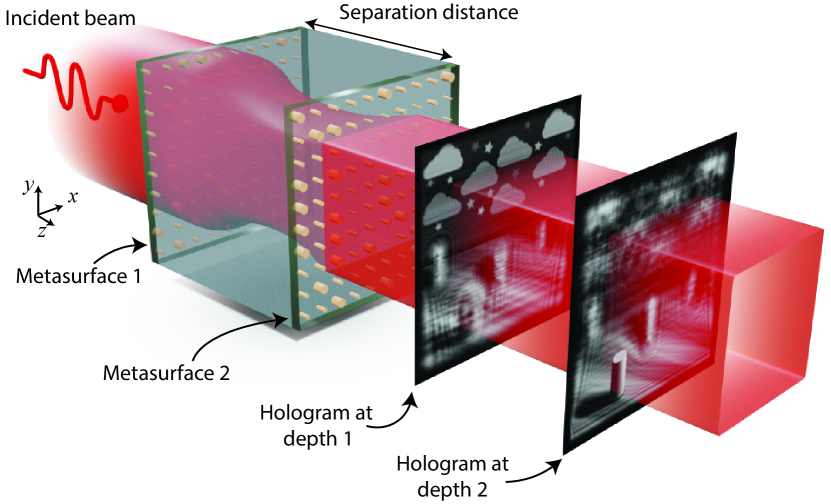
Here, we use two lossless phase-only metasurfaces separated by a short physical distance [20, 21, 22, 23, 24], introduced in [25], to demonstrate amplitude and phase control without relying on loss. This configuration is shown in Fig. 1, and is termed a compound metaoptic [21, 22]. Sequential integration of multiple metasurfaces has allowed aberration correction [26], single-shot phase imaging [27], optical retro-reflection [28], and full-color optical holography [17]. However, the metasurfaces in these cases were each individually designed to implement a particular optical function and then used sequentially. Our method iteratively designs the transmission phase profiles of the metasurfaces together. This enables a more synergistic approach to achieving complex wavefront manipulation. It also expands the application space by combining multiple optical functions into one compact metaoptic device.
Alternative approaches have been developed to optimize cascaded metasurfaces for spatial complex-valued control over a wave. A method to design cascaded metasurfaces for a variety of optical functions was presented in [29]. This method uses adjoint optimization to optimize a sequence of metasurfaces to perform desired field transformations from input to output. A metasurface consisting of cascaded impedance sheets was designed in [30] using waveguide modes to form desired aperture fields through mode conversion at microwave frequencies. Alternative methods to optimize paired metasurfaces, primarily for radiation pattern applications at microwave frequencies, have been shown in [20, 23, 24]. Cascaded diffractive layers have been designed using deep-learning methods to implement all-optical diffractive deep neural networks to perform a variety of detection and classification functions, as well as logic operations [31, 32, 33].
In this paper, we first demonstrate an optical component where a beam-splitter and beam-former are combined into one lossless device. Specifically, an incident uniform illumination is manipulated to form multiple output beams, where peak intensity, propagation angle, and size of each beam is customized. Single-layer metasurfaces have shown beam-splitting based on polarization-dependent phase gradients [34], interleaved gradient phase profiles [12], or forming diffraction orders from phase gratings [35, 36]. However, the output beams were not shaped and the devices exhibited diffraction losses. A reflective metasurface at microwave frequencies [16] demonstrated a beam-splitting/forming function, but used polarization loss to form the complex-valued interference pattern of the desired beam profiles.
In a second example, we design a compound metaoptic to form a three-dimensional computer generated hologram. Creating an exact complex-valued output field is necessary to precisely replicate the 3D scene with optical fields [5, 15, 6]. The advantage of phase-only holograms (single metasurface) is high transmission efficiency, but the image is degraded by the introduction of image speckle. Complex-valued holograms can restore image quality, but at the expense of a lower efficiency if loss is used to control amplitude [5, 15, 6, 13, 17]. Here, we show that the metaoptic platform exhibits high efficiency and produces high-quality images.
In each example, we provide full-wave finite difference time domain (FDTD) simulation results which verify the desired performance. These demonstrations show that compound metaoptics can broaden the application space in a variety of optical functions while maintaining a high overall efficiency.
II Metaoptic Design Procedure
Compound metaoptics are collections of individual metasurfaces arranged along a common axis, analogous to an optical compound lens [22]. The additional degrees of freedom afforded by a multi-metasurface design enables electromagnetic functionalities not possible with a single metasurface. Here, we describe compound metaoptics at a near-infrared wavelength that implement beam-former/splitters and a 3D computer-generated hologram. Two metasurfaces are used to provide the required degrees of freedom to reshape the amplitude and phase profile of a wavefront.
The two reflectionless metasurfaces are arranged sequentially as shown in Fig. 1. The metasurfaces operate in tandem to re-shape the incident wave into a desired amplitude and phase profile transmitted through the metaoptic. In this configuration, the first metasurface forms the correct amplitude profile at the specified separation distance, and the second metasurface provides a phase correction to produce the desired complex-valued field. High efficiency is achieved by re-arranging the power density of the wave from input to output instead of using loss to form the desired field pattern. By requiring the metasurfaces to be reflectionless and lossless, there is no imposed upper limit to the device efficiency.
Designing a compound metaoptic involves defining the incident and output fields, optimizing the metasurface transmission phase shift, and determining the metasurface unit cell design to implement the desired phase shift. In this section, we discuss how these different elements were considered in the design of a compound metaoptic.
II.1 Phase Profile Design
Each metasurface imposes a phase discontinuity on the incident wave, working together to transform a known source field into a desired field profile with specified amplitude and phase distributions. Here, we assume that all field profiles and phase discontinuities are functions of the transverse metasurface dimensions and are spatially inhomogeneous in general. The metasurfaces are polarization-insensitive, so only scalar fields are considered for simplicity. A time convention of is assumed.
The first step in designing a compound metaoptic is to define the incident source and the desired output field distributions. The desired field profile should be scaled in amplitude to conserve the global power contained in the incident field. This is done by multiplying the desired field profile by the square root of the total power ratio
| (1) |
where is the original defined desired field profile. In (1), it was assumed that the field profiles are recorded in the same medium.
For an incident wave defined by its electric field profile , the first metasurface applies a phase discontinuity . The field transmitted through the first metasurface becomes
| (2) |
This transmitted field is decomposed into its plane wave spectrum using the Fourier Transform, and numerically propagated across the separation distance to the second metasurface. The first metasurface is designed to project the desired amplitude profile onto the second metasurface. However, the phase profile here is incorrect relative to the desired field. The second metasurface provides a phase discontinuity to correct the phase error, forming the desired output field in both amplitude and phase. This propagation sequence can be written as
| (3) |
where denotes the Fourier Transform over the and dimensions, represents the wavenumber component in the normal direction for each plane wave component, is the separation distance, and is the spatial phase discontinuity of the second metasurface.
From (2) and (3), it is apparent that two separate phase-discontinuity profiles can form a desired complex-valued field profile without loss. However, determining the profiles implemented by each metasurface is not intuitive and is unlikely to follow a mathematical function.
A phase-retrieval algorithm based on the Gerchberg-Saxton algorithm [37] is used to determine the phase discontinuity implemented by each metasurface. If the amplitude profile of a beam is known at two planes, a phase-retrieval algorithm enables calculation of the phase profile. Since the phase discontinuity planes are assumed to be lossless, the amplitude profiles of the wave at each metasurface are the source and desired amplitude profiles. Since the phase profiles are a free parameter (implemented by each metasurface) they can be calculated so propagation over the separation distance links the two amplitude distributions. As a result, the power density of the incident wave can be redistributed as desired. Other approaches using the adjoint optimization method [29], directly optimizing the plane wave spectrum [20, 23], and optimizing the equivalent electric and magnetic currents of the metasurfaces [24] have been used as well.
The modified Gerchberg-Saxton algorithm used here optimizes the phase profile produced by the first metasurface to form the desired amplitude pattern. However, a direct optimization between the two amplitude profiles might not produce the most accurate result if they are significantly different. This is especially the case if either amplitude profile has a steep change in intensity over a short distance. We employ a more incremental optimization approach to spread the difference in amplitude profiles over a series of phase-retrieval algorithm steps. Specifically, the adjusted amplitude profile fed to each phase-retrieval algorithm instance is a weighted average of the source amplitude profile and the overall desired amplitude profile. The adjusted amplitude () profile is updated between each successive call of the phase-retrieval algorithm, calculated as
| (4) |
where increases incrementally from 0 to 1.
Figure 2 shows a flow chart describing this approach. The multi-level input adjustment block applies (4) to the desired amplitude profile. The adjusted field amplitude , source field amplitude , and phase profile are then fed into the phase-retrieval algorithm block. This algorithm updates the phase profile so that the source field forms the adjusted field amplitude. The updated phase profile is then used as the initial phase estimate during the next adjusted amplitude iteration.
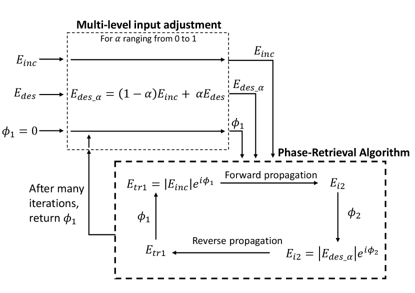
The phase-retrieval algorithm is employed to optimize the phase profile of metasurface 1, so that the desired amplitude profile will be formed at metasurface 2. Figure 2 provides a flowchart summarizing the steps for each iteration. In an iteration, an initial estimate of the phase profile is applied to the incident field. This forms a complex-valued field transmitted by the first metasurface . The field distribution is then decomposed into its plane wave spectrum, where a spectral filter is applied to keep only a range of the spectrum. This spectrum is propagated across the separation distance to the second metasurface by applying the appropriate phase delays [38], and converted to the spatial domain. A new field distribution at metasurface 2 is formed by replacing the propagated field amplitude with the desired amplitude distribution, but retaining the phase profile . The new field distribution is decomposed into its plane wave spectrum, and the spectral filter applied. The plane wave spectrum is then reverse propagated back to the first metasurface and converted to the spatial domain. The resulting phase profile of this field is used as the phase profile in the next iteration.
As the algorithm progresses, the field profile propagated to the second metasurface increasingly matches the given adjusted amplitude distribution. Once the propagated field amplitude sufficiently matches the adjusted amplitude, the phase-retrieval algorithm is halted and the next input level begins. If all input levels have been completed, then the phase profiles of the field at each metasurface plane and are recorded and the overall algorithm exits. The metasurface phase discontinuity profiles are then calculated as the difference in phase between the tangential fields.
| (5) |
| (6) |
II.2 Metasurface Unit Cell
The implementation of each constituent metasurface is a critical factor in the performance of the metaoptic. Ideally, the metasurfaces should have a high transmittance and provide a locally-variable phase shift spanning the full 0 to phase range. In general, this can be achieved with bianisotropic Huygens’ metasurfaces, which are capable of providing a reflectionless phase shift for all angles of refraction [2, 39, 40, 41]. Access to wide angles of refraction allows drastic changes in the power density profile even over short propagation distances [22]. Bianisotropic Huygens’ metasurfaces have been implemented at microwave frequencies but are difficult to achieve at optical wavelengths with low loss.
Optical metasurfaces have been demonstrated that locally control phase and polarization using high dielectric contrast nanopillars with high efficiency [42]. At near-infrared wavelengths, silicon is a common choice of nanopillar material due to its high permittivity, low loss, and ease of fabrication for planar structures [9]. However, the transmission performance can be angularly-dependent, so most designs are limited to be paraxial.
Here, we implement each metasurface as an array of silicon nanopillars with circular cross-sections. A circular cross-section produces a polarization-independent transmission, but polarization-dependent transmission can be achieved using elliptical cross-sections [43]. The transmission of the inhomogeneous metasurface can be modeled by assuming the local periodicity approximation for each unit cell. This approximation has been commonly used and verified at microwave frequencies [44, 45] and optical wavelengths [46, 47].
Various full-wave optimization procedures have been developed to account for interactions between non-identical unit cells in inhomogeneous metasurfaces. These procedures have utilized adjoint optimization of the full metasurface [48] and piece-wise optimization of the metasurface [49] to improve performance. This is particularly useful when large angles of refraction are created by the metasurface (e.g. large numerical aperture lenses). These methods could be utilized in the metaoptic design to improve the overall performance. However, this is beyond the scope of this paper.
The operating wavelength is , and the silicon pillars are placed at a spacing of with a height of . The metasurfaces are assumed to be on the surface of a fused silica substrate and embedded in a layer of PDMS. Similar structures have been successfully fabricated in [26, 28], or as two aligned individually-fabricated metasurfaces [50, 13]. The unit cell geometry is shown in Fig. 3(a). The index of refraction for the various materials was assumed to be for silicon [51], for PDMS, and for fused silica [52].
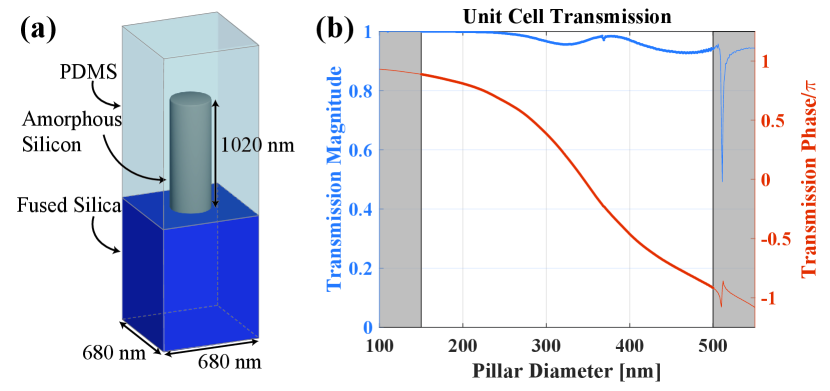
Plane wave transmission by this unit cell as a function of pillar diameter was simulated using the commercial electromagnetic solver Ansys HFSS assuming periodic boundaries. As shown in Fig. 3(b), a radian transmission phase shift range (90.5% phase coverage) is achieved for pillar diameters ranging from to , with transmission magnitude above 0.93.
Two metasurfaces of silicon nanopillar unit cells are used to form the compound metaoptics, since they can provide a desired local phase shift while maintaining high transmission. However, this metasurface implementation has practical limitations that must be accounted for to obtain optimal performance from the metaoptic.
II.3 Unit Cell Induced Design Restrictions
A number of design constraints are imposed by the choice of the metasurface unit cell used here. In [22], we describe a compound metaoptic implemented with bianisotropic Huygens’ metasurfaces. Bianisotropy allows reflectionless wide-angle refraction by impedance matching the incident wave to the transmitted wave [53, 41]. The silicon nanopillars considered here do not exhibit bianisotropy, and cannot implement reflectionless wide-angle refraction. This fundamental difference results in design limitations that must be accounted for.
The main restriction is that the transmission phase of the silicon pillars changes as the angle of incidence changes. To mitigate this, we allow the metasurface phase shift to produce a transmitted field containing only plane wave components with angles less than degrees. This corresponds to allowing transverse wavenumber components of
| (7) |
where is the transverse wavenumber of the plane wave spectrum and is the free space wavenumber.
The ability to reshape the power density profile is reduced for a given separation distance when the available plane wave spectrum is restricted. Distributing the power density of a source into a significantly different pattern requires a wider spectrum for shorter separation distances. Since the available spectral region is limited by the metasurface implementation, the design parameters must modified. Two options are available: the desired field amplitude pattern can be made more similar to the source distribution, or the separation distance between metasurfaces can be increased. Increasing the separation distance is more palatable since it maintains the ability to form the desired amplitude distribution. Doing so can also provide structural integrity if a rigid substrate (handle wafer) is used as the separation distance medium.
By limiting the angular spread of the plane-wave spectrum, the wave impedance of the fields tangential to the metasurface plane is approximately equal to the characteristic impedance of the medium. Therefore, the power density of the wavefront can be accurately approximated as the square of the electric field amplitude. The power density conservation requirement at each metasurface simplifies to conserving the amplitude of the electric field with a scalar dependent on the material parameters. Since only the amplitude distribution needs to be considered, the number of calculations required in the optimization is reduced.
With these considerations in mind, metaoptics can be designed to perform different optical functions.
III Simulation Results
In this section we discuss two examples of metaoptics performing different functions: optical beam-forming and splitting, and displaying a three-dimensional hologram. These cases use different methods to calculate the desired output field. The beam-former/splitter output field is defined by direct summation of the output beams. The 3D hologram output field is formed by manipulating the plane wave spectrum representation of flat images to provide depth to the hologram scene [54, 55, 56].
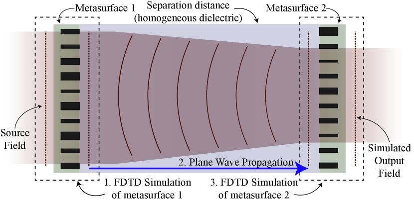
In each case, the metasurfaces are arrays of silicon pillars, separated by a distance of of fused silica. The metasurface parameters are calculated using the metaoptic design process outlined in Section II.1. Simulations of the resulting metasurface nanopillar distributions were performed with the open-source finite difference time-domain (FDTD) EM solver MEEP [57]. The simulations account for the inhomogeneous pillar distribution of the metasurface, and the resulting effects on the transmitted field distribution. However, it is impractical to simulate the entire metaoptic due to the optically large separation distance. Since the separation distance is filled by a homogeneous dielectric, the simulated electric field distribution transmitted by metasurface 1 can be numerically propagated to metasurface 2 using the plane wave spectrum without loss of accuracy. By combining these two features, a hybrid simulation approach can be taken to accurately simulate the overall performance of the metaoptic.
Figure 4 shows a diagram of simulation steps to determine the performance for each metaoptic. First, the transmitted field distribution is recorded from an FDTD simulation of metasurface 1 using the known source field as the illumination. Second, this transmitted field is numerically propagated across the separation distance using the plane wave spectrum. Finally, this propagated field is used as the illumination for an FDTD simulation of metasurface 2, where the transmitted field profile is recorded. This simulated output field is compared to the expected field distribution to evaluate the overall performance of the metaoptic. For each example, the full-wave simulation results for each metasurface and a comparison to a version with phase-only control (desired phase profile applied to the incident amplitude) are given in the supplementary material [58]. Reflections from each metasurface are assumed to be very small due to the unit cell design, so any interaction between metasurfaces is ignored. Full-wave simulations confirm low reflections from each metasurface, validating this assumption.
III.1 Beam-former/splitter
The beam-former/splitter metaoptic is designed to convert a uniform illumination into multiple desired output beams. Such a device would be useful in optical tweezer applications, where particle manipulation can require unique amplitude and phase profiles of laser beams [7]. Beam-splitter metasurfaces have been designed to form multiple output beams in previous work. However the amplitude profiles of the split beams were not altered, and losses to diffraction orders were present [12, 34, 35, 36].
Here, we demonstrate reshaping an incident circular uniform illumination into multiple output beams with different beam widths and propagation angles. The complex-valued interference pattern of the beams is formed at the output of the device. By doing so, all available power from the source distribution is redirected into the desired output beams. Two examples are described: an in-plane beam-splitter with two output beams, and a multi-beam splitter with seven output beams.
III.1.1 In-Plane Beam-Former/Splitter
The first metaoptic example forms two output Gaussian beams with different beam widths and relative amplitudes from a circular uniform illumination. When only two output Gaussian beams are formed, a plane can be drawn containing the propagation direction of both beams, constituting an in-plane beam-former/splitter. An aperture window can be placed around metasurface 1 to form the uniform illumination from an incident beam over-filling the device. We describe this illumination across metasurface 1 as having a uniform phase and amplitude, . The output field is calculated from the direct sum of the desired beams, forming a complex-valued interference pattern. Beam 1 has a beam radius of , peak relative intensity of 0.5, and propagation angle of . Beam 2 has a radius of , a relative peak intensity of 1, and propagation angle of . The desired output field is define as
| (8) |
where the Gaussian beams are defined as
| (9) | ||||
| (10) |
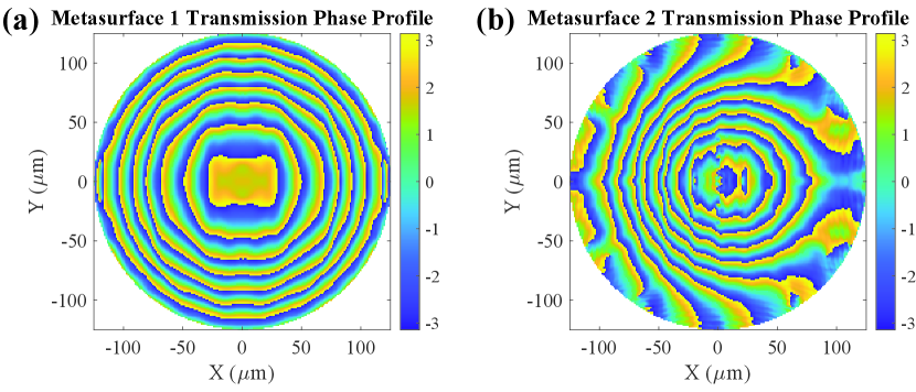
The phase discontinuity profiles forming the desired output field are calculated with the metaoptic design process described in Section II.1 and are shown in Fig. 5. These phase profiles are sampled at the unit cell periodicity and converted to pillar diameter distributions using the relationship in Fig. 3(b). The silicon pillar array of metasurface 1 is then simulated in MEEP to obtain the transmitted field across the entire metasurface.
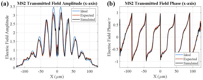
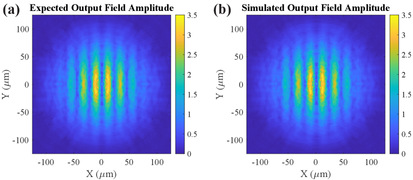
This field is propagated across the separation distance and used as the illuminating field for the FDTD simulation of metasurface 2. The resulting amplitude profile of the transmitted field is shown in Fig. 6. The simulated output field amplitude matches the desired field profile defined in (8). Figure 7 shows the electric field amplitude and phase along the -axis, where the simulated field profiles closely match the desired profiles.
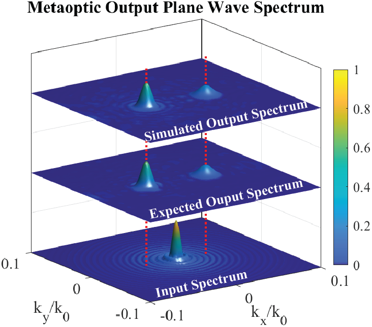
Since the propagation characteristics of a field distribution are defined by its plane wave spectrum, we can use the output field spectrum to evaluate the simulated performance of the metaoptic. Figure 8 compares the plane wave spectrum for the input, expected output, and simulated output field distributions of the metaoptic (normalized to the input spectrum peak magnitude). We see that the desired beams are created at the correct spectral locations and with very little spectral noise. There is no trace of the input field spectrum at the output. This signifies that the source field distribution has been accurately reshaped in amplitude and phase to the desired complex-valued output field.
The overall efficiency of the in-plane beam-splitter device was calculated from the simulations to be 81%. The efficiency is defined as the percentage of input power (in the uniform illumination) contained in the two output Gaussian beams. The majority of the lost power is due to the minor reflections (about 8% per metasurface) incurred by the metasurface implementation using silicon pillars, with the remainder lost to spectral noise. However, the overall efficiency of the device is still very high.
| Beam | Relative Intensity | (degrees) | (degrees) |
|---|---|---|---|
| 1 | 1 | 1.75 | 1.8 |
| 2 | 1 | -1.75 | 1.8 |
| 3 | 0.7 | -2.25 | -1.6 |
| 4 | 0.7 | -0.8 | -2.45 |
| 5 | 0.7 | 0.8 | -2.45 |
| 6 | 0.7 | 2.25 | -1.6 |
III.1.2 Multi-Beam Former/Splitter
The multi-beam former/splitter converts a uniform illumination into multiple output beams propagating in different directions in space. Here, six Gaussian beams and one Bessel beam are formed from a uniform circular illumination as a demonstration. The output field profile is calculated as the direct sum of the different beams, and varies in both lateral dimensions of the metaoptic output. The desired field profile is defined as
| (11) | ||||
where denotes the zeroth-order Bessel function, is the radial distance from the center of the metasurface, and the values for , , and are given in Table 1.
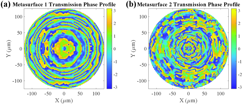
The phase discontinuity profiles of the constituent metasurfaces are calculated using the design procedure, and are shown in Fig. 9. The phase profiles are translated into a distribution of silicon nanopillars to implement each metasurface and simulated to obtain the output field distribution of the metaoptic.
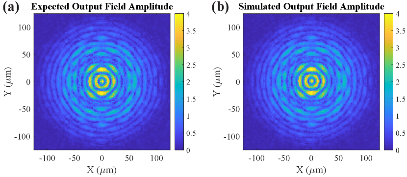
The multi-stage FDTD simulation approach was again used to determine the output field profile of the metaoptic. The simulated output electric field amplitude is shown in Fig. 10, which appears nearly identical to the expected output field amplitude.
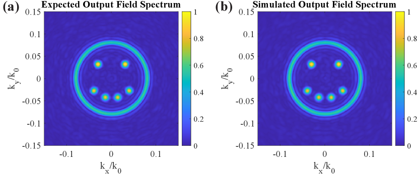
To demonstrate that the simulated metaoptic output field is correct in both amplitude and phase, the plane wave spectrum is observed to show the presence of each constituent beam. Figure 11 shows the plane wave spectra of the simulated output field distribution, where we see the characteristic annulus of the Bessel beam and the six Gaussian beams arranged at the desired spectral locations. The input source field is completely converted to the multiple desired output beams with very little spectral noise and no undesired diffraction orders. This shows that multiple beams can be formed exactly, without loss, from a given source field profile.
The overall efficiency of the multi-beam former/splitter was calculated from simulations to be 78%. The efficiency is defined as the percentage of input power contained in the output beams. While still a high efficiency, the majority of the lost power occurs from slight reflections from each metasurface (about 10% per metasurface) and power lost to spectral noise.
III.2 3D Hologram
Holography is a process in which optical fields are constructed in amplitude and phase for the purpose of forming an image. Computer-generated holography (CGH) is a technique to generate the complex-valued fields forming a 3D scene using numerical calculation rather than by direct capture of scattered light [59]. The result is a 2D complex-valued field distribution at one plane which contains the information to produce the desired 3D scene.
Many approaches have been taken to produce holograms using metasurfaces [60]. In particular, a variety of approaches have been shown to form complex-valued holograms, which result in high-quality images. However, these approaches utilize loss in the form of polarization conversion to achieve amplitude control [5, 14, 15, 6, 16, 17], thereby limiting the efficiency. In contrast, compound metaoptics produce desired complex-valued output fields without loss, providing the desired capability to form high-quality 3D holograms with high efficiency.
In this example, the field profile of the hologram is engineered using CGH methods and implemented using the metaoptic design process. This demonstrates the value of using metaoptics to accurately form a desired output field for holographic display applications. Phase-only holograms provide a simple approach to forming a desired hologram, but suffer from image quality reduction. Controlling the amplitude and phase of the output field avoids these issues [6], and can be directly implemented in a lossless manner with compound metaoptics.
Many methods have been used to visually approximate depth in a 3D CGH, differentiated by the sampling approach of the scene [59]. More simplistic approaches are modelling the objects as a cloud of point sources, or collapsing a 3D scene into 2D images at different depths. These methods reduce the required computation but image quality suffers due to reduced sampling of the 3D surface. More complicated approaches are methods which track ray interactions with the object to approximate scattering characteristics, and methods that form the 3D scene from a surface mesh of polygons with defined amplitude distributions. The hologram quality can be improved at the expense of calculation complexity.
For the metaoptic hologram example, we utilized a polygon surface mesh method to form a simple 3D scene [54, 55, 56]. This approach is outlined in the supplemental material [58]. The hologram is formed from an ensemble of image components arranged in a 3D scene. Occlusion of one image component by another is accounted for to present each image as solid, preventing background images from leaking through foreground objects. The compound metaoptic provides a high-quality realistic representation of a 3D scene.
III.2.1 Output Field Design
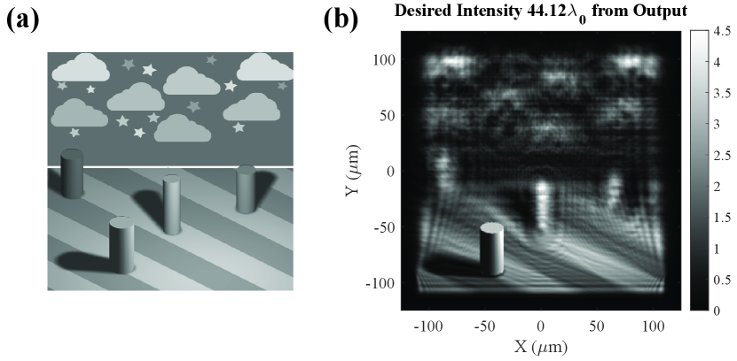
The output field of the compound metaoptic is designed to form a 3D scene with multiple image components: a background image, a floor image, and four cylinders. Shadows cast by the cylinders from a localized light source are overlaid on the floor image, providing the appearance of a simple real-world scene. A series of steps is taken to combine the hologram components into a single amplitude and phase profile to be formed by the metaoptic. Figure 12(a) shows a diagram of the scene, viewed from a elevation angle of 30 degrees.
The total 3D hologram scene is scaled to cover 90% of the metaoptic aperture size, so that it is in dimension. Each image component was converted to an electric field distribution and added to the total aperture field distribution. The background and floor images were added to the total field profile first, and then each cylinder added from back to front. The hologram component images were rotated in space to provide the desired vantage point by applying a coordinate rotation to the plane wave spectrum of each image [59, 55, 54, 56].
Finally, the entire hologram field is shifted so that the middle of the 3D scene is in focus at the metaoptic output. As a result, half the hologram comes into focus when imaging a depth behind the output, and half is in focus when imaging a depth in front of the output. Fig. 12(b) shows the ideal hologram intensity focused on the forward-most cylinder.
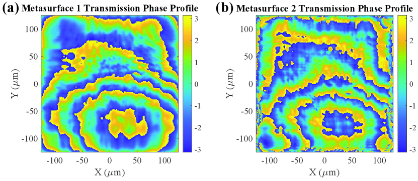
The metasurface phase shift profiles that transform the uniform square illumination into the 3D hologram are shown in Fig. 13. The phase shift profiles are sampled and translated to silicon pillar distributions, which were then simulated to evaluate the metaoptic performance.
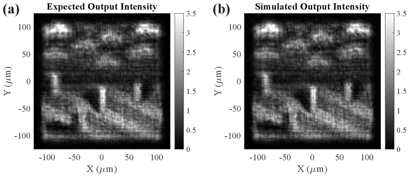
The expected output intensity formed by the metaoptic is shown in Fig. 14(a). By simulating the metasurfaces with the hybrid FDTD approach, the output intensity is obtained and shown in Fig. 14(b). We see that the simulated output intensity distribution closely matches the expected output intensity. Therefore, the metasurfaces faithfully implement the phase planes and will accurately produce the 3D hologram scene.
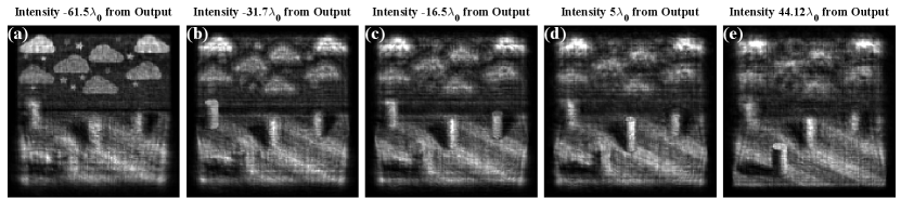
To demonstrate depth of the 3D hologram, the simulated output field profile was numerically propagated to different depths to image different locations of the 3D hologram. The depths are determined so that each image has the background or one of the cylinders in focus, while the other components are out of focus. The depths of each image plane relative to the output plane are given in Table 2, where the cylinders are numbered from back to front. These images are shown in Fig. 15 and demonstrate the 3D nature of the hologram scene formed by the compound metaoptic.
| Hologram Component | Depth Relative to Metaoptic Output |
|---|---|
| Background | |
| Cylinder 1 | |
| Cylinder 2 | |
| Cylinder 3 | |
| Cylinder 4 |
The simulated 3D hologram clearly shows that compound metaoptics can be designed to produce high-quality computer-generated holograms. Since the desired hologram images are formed at multiple planes with high quality, this signals that the output field amplitude and phase distributions have been accurately produced by the metaoptic. Furthermore, loss was not relied upon to shape the amplitude pattern, so the hologram was formed with an efficiency of 86% as determined from simulations. Slight reflections from the metasurfaces account for most of the lost power (about 6% per metasurface) with the rest lost to spectrum noise.
IV Conclusion
Overall, we have shown how compound metaoptics can reshape the amplitude and phase profile of a source field distribution, without loss, to perform a variety of optical functions. Two lossless phase-discontinuous metasurfaces are used to construct the metaoptic, which leads to high overall efficiency. In contrast, amplitude and phase manipulations by single metasurfaces use loss to form the spatial amplitude profile.
We demonstrated how compound metaoptics can be used to perform a variety of optical functions. Two metaoptics exhibiting a combined beam-forming and beam-splitting function were designed to reshape a uniform illumination into multiple output beams. Another metaoptic demonstrated that 3D holograms can be formed from a uniform illumination with high image quality. The metaoptics were designed at a near-infrared wavelength and full-wave simulation results show that their performance matched desired expectations in each case with high efficiency.
The results show that the metaoptic design process can accurately reshape a given source field distribution into an arbitrary complex-valued output field distribution. With the compound metaoptic approach, the advantages of lossless field manipulation and a small physical size can be combined into a single device. Such compound metaoptics could lead to improved performance in three-dimensional holography, compact holographic displays and custom optical elements, and micro particle manipulation with optical tweezers.
Acknowledgements.
This research was supported by the National Science Foundation Graduate Research Fellowship Program and the Office of Naval Research under Grant No. N00014-18-1-2536. This research was supported in part through computational resources and services provided by Advanced Research Computing at the University of Michigan, Ann Arbor.References
- Khorasaninejad et al. [2016] M. Khorasaninejad, W. T. Chen, R. C. Devlin, J. Oh, A. Y. Zhu, and F. Capasso, Metalenses at visible wavelengths: Diffraction-limited focusing and subwavelength resolution imaging, Science 352, 1190 (2016).
- Pfeiffer and Grbic [2013a] C. Pfeiffer and A. Grbic, Metamaterial Huygens’ Surfaces: Tailoring Wave Fronts with Reflectionless Sheets, Physical Review Letters 110, 197401 (2013a).
- Pfeiffer et al. [2014a] C. Pfeiffer, N. K. Emani, A. M. Shaltout, A. Boltasseva, V. M. Shalaev, and A. Grbic, Efficient Light Bending with Isotropic Metamaterial Huygens’ Surfaces, Nano Letters 14, 2491 (2014a).
- Chong et al. [2016] K. E. Chong, L. Wang, I. Staude, A. R. James, J. Dominguez, S. Liu, G. S. Subramania, M. Decker, D. N. Neshev, I. Brener, and Y. S. Kivshar, Efficient Polarization-Insensitive Complex Wavefront Control Using Huygens’ Metasurfaces Based on Dielectric Resonant Meta-atoms, ACS Photonics 3, 514 (2016).
- Wang et al. [2016] Q. Wang, X. Zhang, Y. Xu, J. Gu, Y. Li, Z. Tian, R. Singh, S. Zhang, J. Han, and W. Zhang, Broadband metasurface holograms: toward complete phase and amplitude engineering, Scientific Reports 6, 1 (2016).
- Overvig et al. [2019] A. C. Overvig, S. Shrestha, S. C. Malek, M. Lu, A. Stein, C. Zheng, and N. Yu, Dielectric metasurfaces for complete and independent control of the optical amplitude and phase, Light: Science & Applications 8, 1 (2019).
- Jesacher et al. [2008a] A. Jesacher, C. Maurer, A. Schwaighofer, S. Bernet, and M. Ritsch-Marte, Full phase and amplitude control of holographic optical tweezers with high efficiency, Optics Express 16, 4479 (2008a).
- Yu and Capasso [2014] N. Yu and F. Capasso, Flat optics with designer metasurfaces, Nature Materials 13, 139 (2014).
- Staude and Schilling [2017] I. Staude and J. Schilling, Metamaterial-inspired silicon nanophotonics, Nature Photonics 11, 274 (2017).
- He et al. [2018] Q. He, S. Sun, S. Xiao, and L. Zhou, High-Efficiency Metasurfaces: Principles, Realizations, and Applications, Advanced Optical Materials 6, 1800415 (2018).
- Kwon et al. [2018] D.-H. Kwon, G. Ptitcyn, A. Diaz-Rubio, and S. A. Tretyakov, Transmission Magnitude and Phase Control for Polarization-Preserving Reflectionless Metasurfaces, Physical Review Applied 9, 034005 (2018).
- Zhang et al. [2018a] D. Zhang, M. Ren, W. Wu, N. Gao, X. Yu, W. Cai, X. Zhang, and J. Xu, Nanoscale beam splitters based on gradient metasurfaces, Optics Letters 43, 267 (2018a).
- Zhou et al. [2019] Y. Zhou, I. I. Kravchenko, H. Wang, H. Zheng, G. Gu, and J. Valentine, Multifunctional metaoptics based on bilayer metasurfaces, Light: Science & Applications 8, 1 (2019).
- Li et al. [2016] Z. Li, H. Cheng, Z. Liu, S. Chen, and J. Tian, Plasmonic Airy Beam Generation by Both Phase and Amplitude Modulation with Metasurfaces, Advanced Optical Materials 4, 1230 (2016).
- Lee et al. [2018] G.-Y. Lee, G. Yoon, S.-Y. Lee, H. Yun, J. Cho, K. Lee, H. Kim, J. Rho, and B. Lee, Complete amplitude and phase control of light using broadband holographic metasurfaces, Nanoscale 10, 4237 (2018).
- Bao et al. [2019] L. Bao, R. Y. Wu, X. Fu, Q. Ma, G. D. Bai, J. Mu, R. Jiang, and T. J. Cui, Multi-Beam Forming and Controls by Metasurface With Phase and Amplitude Modulations, IEEE Transactions on Antennas and Propagation 67, 6680 (2019).
- Huang et al. [2020] X. Huang, S. Shrestha, A. Overvig, and N. Yu, Three-color phase-amplitude holography with a metasurface doublet, in 2020 Conference on Lasers and Electro-Optics (CLEO) (2020) pp. 1–2.
- Jesacher et al. [2008b] A. Jesacher, C. Maurer, A. Schwaighofer, S. Bernet, and M. Ritsch-Marte, Near-perfect hologram reconstruction with a spatial light modulator, Optics Express 16, 2597 (2008b).
- Wu et al. [2018] C. Wu, J. Ko, J. R. Rzasa, D. A. Paulson, and C. C. Davis, Phase and amplitude beam shaping with two deformable mirrors implementing input plane and Fourier plane phase modifications, Applied Optics 57, 2337 (2018).
- Dorrah and Eleftheriades [2018] A. H. Dorrah and G. V. Eleftheriades, Bianisotropic Huygens’ Metasurface Pairs for Nonlocal Power-Conserving Wave Transformations, IEEE Antennas and Wireless Propagation Letters 17, 1788 (2018).
- Raeker et al. [2019] B. O. Raeker, A. Grbic, Y. Zhou, and J. Valentine, All-Dielectric Compound Metaoptics, in 2019 IEEE International Symposium on Antennas and Propagation and USNC-URSI Radio Science Meeting (2019) pp. 431–432.
- Raeker and Grbic [2019] B. O. Raeker and A. Grbic, Compound metaoptics for amplitude and phase control of wave fronts, Phys. Rev. Lett. 122, 113901 (2019).
- Ataloglou et al. [2020] V. G. Ataloglou, A. H. Dorrah, and G. V. Eleftheriades, Design of compact huygens’ metasurface pairs with multiple reflections for arbitrary wave transformations, IEEE Transactions on Antennas and Propagation (2020).
- Brown and Mojabi [2020] T. Brown and P. Mojabi, Cascaded metasurface design using electromagnetic inversion with gradient-based optimization, TechRxiv (2020).
- Raeker and Grbic [2018] B. O. Raeker and A. Grbic, Paired Metasurfaces for Amplitude and Phase Control of Wavefronts, in 2018 IEEE International Symposium on Antennas and Propagation USNC/URSI National Radio Science Meeting (2018) pp. 1479–1480.
- Arbabi et al. [2016] A. Arbabi, E. Arbabi, S. M. Kamali, Y. Horie, S. Han, and A. Faraon, Miniature optical planar camera based on a wide-angle metasurface doublet corrected for monochromatic aberrations, Nature Communications 7, 1 (2016).
- Kwon et al. [2020] H. Kwon, E. Arbabi, S. M. Kamali, M. Faraji-Dana, and A. Faraon, Single-shot quantitative phase gradient microscopy using a system of multifunctional metasurfaces, Nature Photonics 14, 109 (2020).
- Arbabi et al. [2017] A. Arbabi, E. Arbabi, Y. Horie, S. M. Kamali, and A. Faraon, Planar metasurface retroreflector, Nature Photonics 11, 415 (2017).
- Backer [2019] A. S. Backer, Computational inverse design for cascaded systems of metasurface optics, Opt. Express 27, 30308 (2019).
- Alsolamy and Grbic [2020] F. Alsolamy and A. Grbic, Cylindrical aperture synthesis with metasurfaces, in 2020 14th European Conference on Antennas and Propagation (EuCAP) (2020) pp. 1–2.
- Lin et al. [2018] X. Lin, Y. Rivenson, N. T. Yardimci, M. Veli, Y. Luo, M. Jarrahi, and A. Ozcan, All-optical machine learning using diffractive deep neural networks, Science 361, 1004 (2018).
- Mengu et al. [2020] D. Mengu, Y. Zhao, N. T. Yardimci, Y. Rivenson, M. Jarrahi, and A. Ozcan, Misalignment resilient diffractive optical networks, Nanophotonics 9, 4207 (01 Oct. 2020).
- Qian et al. [2020] C. Qian, X. Lin, X. Lin, J. Xu, Y. Sun, E. Li, B. Zhang, and H. Chen, Performing optical logic operations by a diffractive neural network, Light: Science & Applications 9 (2020).
- Li et al. [2019] J. Li, C. Liu, T. Wu, Y. Liu, Y. Wang, Z. Yu, H. Ye, and L. Yu, Efficient Polarization Beam Splitter Based on All-Dielectric Metasurface in Visible Region, Nanoscale Research Letters 14, 34 (2019).
- Zhang et al. [2018b] X. Zhang, R. Deng, F. Yang, C. Jiang, S. Xu, and M. Li, Metasurface-Based Ultrathin Beam Splitter with Variable Split Angle and Power Distribution, ACS Photonics 5, 2997 (2018b).
- Lin et al. [2019] Y. Lin, M. Wang, Z. Sui, Z. Zeng, and C. Jiang, Highly efficient beam splitter based on all-dielectric metasurfaces, Japanese Journal of Applied Physics 58, 060918 (2019).
- Gerchberg and Saxton [1972] R. Gerchberg and W. Saxton, A practical algorithm for the determination of phase from image and diffraction plane pictures, Optik 35, 237 (1972).
- Goodman [2017] J. W. Goodman, Introduction to Fourier optics, 4th ed. (W.H. Freeman and Company, 2017).
- Pfeiffer and Grbic [2014] C. Pfeiffer and A. Grbic, Bianisotropic metasurfaces for optimal polarization control: Analysis and synthesis, Phys. Rev. Applied 2, 044011 (2014).
- Pfeiffer et al. [2014b] C. Pfeiffer, C. Zhang, V. Ray, L. J. Guo, and A. Grbic, High performance bianisotropic metasurfaces: Asymmetric transmission of light, Phys. Rev. Lett. 113, 023902 (2014b).
- Wong et al. [2016] J. P. S. Wong, A. Epstein, and G. V. Eleftheriades, Reflectionless Wide-Angle Refracting Metasurfaces, IEEE Antennas and Wireless Propagation Letters 15, 1293 (2016).
- Kamali et al. [2018] S. M. Kamali, E. Arbabi, A. Arbabi, and A. Faraon, A review of dielectric optical metasurfaces for wavefront control, Nanophotonics 7, 1041 (2018).
- Arbabi et al. [2015] A. Arbabi, Y. Horie, M. Bagheri, and A. Faraon, Dielectric metasurfaces for complete control of phase and polarization with subwavelength spatial resolution and high transmission, Nature Nanotechnology 10, 937 (2015).
- Pozar et al. [1997] D. M. Pozar, S. D. Targonski, and H. D. Syrigos, Design of millimeter wave microstrip reflectarrays, IEEE Transactions on Antennas and Propagation 45, 287 (1997).
- Fong et al. [2010] B. H. Fong, J. S. Colburn, J. J. Ottusch, J. L. Visher, and D. F. Sievenpiper, Scalar and tensor holographic artificial impedance surfaces, IEEE Transactions on Antennas and Propagation 58, 3212 (2010).
- Pfeiffer and Grbic [2013b] C. Pfeiffer and A. Grbic, Cascaded metasurfaces for complete phase and polarization control, Applied Physics Letters 102, 231116 (2013b).
- Pestourie et al. [2018] R. Pestourie, C. Pérez-Arancibia, Z. Lin, W. Shin, F. Capasso, and S. G. Johnson, Inverse design of large-area metasurfaces, Opt. Express 26, 33732 (2018).
- Mansouree et al. [2020] M. Mansouree, H. Kwon, E. Arbabi, A. McClung, A. Faraon, and A. Arbabi, Multifunctional 2.5D metastructures enabled by adjoint optimization, Optica 7, 77 (2020).
- Phan et al. [2019] T. Phan, D. Sell, E. W. Wang, S. Doshay, K. Edee, J. Yang, and J. A. Fan, High-efficiency, large-area, topology-optimized metasurfaces, Light: Science & Applications 8 (2019).
- Zhou et al. [2018] Y. Zhou, I. I. Kravchenko, H. Wang, J. R. Nolen, G. Gu, and J. Valentine, Multilayer Noninteracting Dielectric Metasurfaces for Multiwavelength Metaoptics, Nano Letters 18, 7529 (2018).
- Edwards [1985] D. F. Edwards, Silicon (Si), in Handbook of Optical Constants of Solids, edited by E. D. Palik (Academic Press, Boston, 1985) pp. 547 – 569.
- Philipp [1985] H. R. Philipp, Silicon Dioxide (SiO2) (Glass), in Handbook of Optical Constants of Solids, edited by E. D. Palik (Academic Press, Boston, 1985) pp. 749 – 763.
- Epstein and Eleftheriades [2014] A. Epstein and G. V. Eleftheriades, Passive lossless huygens metasurfaces for conversion of arbitrary source field to directive radiation, IEEE Transactions on Antennas and Propagation 62, 5680 (2014).
- Matsushima [2005] K. Matsushima, Computer-generated holograms for three-dimensional surface objects with shade and texture, Applied Optics 44, 4607 (2005).
- Matsushima and Nakahara [2009] K. Matsushima and S. Nakahara, Extremely high-definition full-parallax computer-generated hologram created by the polygon-based method, Applied Optics 48, H54 (2009).
- Matsushima et al. [2012] K. Matsushima, H. Nishi, and S. Nakahara, Simple wave-field rendering for photorealistic reconstruction in polygon-based high-definition computer holography, Journal of Electronic Imaging 21, 023002 (2012).
- Oskooi et al. [2010] A. F. Oskooi, D. Roundy, M. Ibanescu, P. Bermel, J. D. Joannopoulos, and S. G. Johnson, Meep: A flexible free-software package for electromagnetic simulations by the FDTD method, Computer Physics Communications 181, 687 (2010).
- [58] See supplemental material at [url will be inserted by publisher] for full-wave simulations, comparison to phase-only implementations, and overview of computer-generated hologram method.
- Park [2017] J.-H. Park, Recent progress in computer-generated holography for three-dimensional scenes, Journal of Information Display 18, 1 (2017).
- Huang et al. [2018] L. Huang, S. Zhang, and T. Zentgraf, Metasurface holography: from fundamentals to applications, Nanophotonics 7, 1169 (01 Jun. 2018).