Lorenz System State Stability Identification using Neural Networks
Abstract
Nonlinear dynamical systems such as Lorenz63 equations are known to be chaotic in nature and sensitive to initial conditions. As a result, a small perturbation in the initial conditions results in deviation in state trajectory after a few time steps. System identification is often challenging in such systems especially when the solution transitions from one regime to another compared to identification when the trajectory of the solution resides within the same regime. The algorithms and computational resources needed to accurately identify the system states vary depending on whether the solution is in transition region or not. We refer to the transition and non-transition regions as unstable and stable regions respectively. We label a system state to be stable if it’s immediate past and future states reside in the same regime. However, at a given time step we don’t have the prior knowledge about whether system is in stable or unstable region. In this paper, we develop and train a feed forward (multi-layer perceptron) Neural Network to classify the system states of a Lorenz system as stable and unstable. We pose this task as a supervised learning problem where we train the neural network on Lorenz system which have states labeled as stable or unstable. We then test the ability of the neural network models to identify the stable and unstable states on a different Lorenz system that is generated using different initial conditions. We also evaluate the classification performance in the mismatched case i.e., when the initial conditions for training and validation data are sampled from different intervals. We show that certain normalization schemes can greatly improve the performance of neural networks in especially these mismatched scenarios. The classification framework developed in the paper can be a preprocessor for a larger context of sequential decision making framework where the decision making is performed based on observed stable or unstable states.
I Introduction
Automated decision making in complex systems relies on robust system state identification under uncertainty. System state identification via data-driven learning is the often the first step within a sequential decision making (SDM) framework Amiri, Shirazi, and Zhang (2019). An SDM framework may comprise of multiple computational modules for system state estimation, context-aware reasoning, and probabilistic planning. A computational agent in such settings may continuously interact with an external environment, compute the best policies (state to action mappings), and execute actions that maximize learning reward signals in the long run Sutton and Barto (2018). In this context, system state is often hidden or partially observable from an agent. This requires an agent to infer the state of the system indirectly through a combination of data driven learning and domain knowledge. Typically the system state space can be characterized in discrete terms to represent different operating regimes. A discrete state space representation may result in translation of the state estimation problem as a data-driven classification task. In recent years, use of neural network classifiers have led to high accuracy and performance across multi-modal data streams (for example text and image)He et al. (2015). State estimation of complex systems such as nonlinear dynamical systems (for example Lorenz63 equations) is challenging due to fluctuating system trajectories and high sensitivity to initial conditions. In this paper, we demonstrate a proof of concept application with a neural network classifier for state estimation of a nonlinear chaotic dynamical system.
Neural networks are a sequence of densely interconnected nodes. Through a process known as training, the networks learn the parameters, or the relationship between these nodes. The availability of large amounts of data and massive computational power are some of the reasons that have facilitated training of deep neural networks in recent years. Consequently, deep neural networks have garnered widespread attention across different scientific disciplines including speech recognitionHinton et al. (2012), image classificationHe et al. (2015), language modelingVaswani et al. (2017) and even protein foldingSenior et al. . The idea of leveraging neural networks to study dynamical systems has been explored for many yearsNarendra and Parthasarathy . Recently, both feed-forward and recurrent architectures have been used for several forecasting and prediction based tasks on chaotic systems. For example, feed-forward neural networks have been shown to predict extreme events in Hénon map Lellep et al. (2020) and LSTMHochreiter and Schmidhuber (1997) architectures have been used for forecasting high-dimensional chaotic systems Vlachas et al. . Additionally Reservoir Computing based approaches have been leveraged for data-driven prediction of chaotic systems (Refs. Chattopadhyay, Hassanzadeh, and Subramanian, 2020; Pathak et al., 2018a, b). There is also literature suggesting that a hybrid approach to forecasting involving both machine learning and knowledge based models Pathak et al. (2018a) leads to higher prediction accuracy for a longer period on chaotic systems. Another line of work involves discovering underlying models from data, wherein autoencoder network architectures are used to recognize the coordinate transformation and the governing equations of the dynamical systems Champion et al. (2019). All these examples highlight the general feasibility of using machine learning and neural networks to study a wide variety of tasks involving chaotic systems. Previous work has shown that feed-forward neural networks are reasonable candidates for predicting regime changes and duration in Lorenz63 systems Brugnago et al. (2020). Inspired by this approach, we leverage feed-forward neural networks for our novel task of classifying the data points of Lorenz system. The solution of the Lorenz system consists of two regimes which we refer to as the left and right regimes. Unlike the approach proposed in Brugnago et al., 2020, we do not restrict ourselves to the boundary to distinguish between the left and right regimes. Since we are interested in studying a broader range of Lorenz systems, we adopt the mean value of x-coordinates as a boundary to distinguish between the left and right regimes. Additionally, unlike Brugnago et al., 2020, we do not constrain ourselves to the interval for sampling the initial conditions for the variables for training and validation datasets. Instead, we sample the initial conditions for training and validation datasets from a wide range of intervals (Sections IV.1 and IV.2) and analyze the behaviour of the classifier in these intervals.
One common problem associated with neural network architectures is lack of generalization with validation data that is drawn from a different distribution as compared to the data used for training. This mismatch between training and validation distributions, also referred to as covariate shift Sugiyama and Kawanabe (2012) is a well-studied aspect in most of the scientific fields that have benefited from advances in neural network architectures. For example, within the speech recognition community, this mismatch is referred to as the acoustic mismatch and is one of the most critical factors that affects the deployment of speech recognition systems in real world environments Vincent et al. (2017). A similar terminology used in the field of natural language processing is domain mismatch, which renders tasks like cross-lingual document classification especially challenging Lai et al. (2019). In the context of chaotic systems, there has been some published work Scher and Messori (2019) that discusses the generalization capabilities of neural networks trained on Lorenz systems. One of the results of this work on Lorenz63 systems is that neural networks trained only on a part of the system’s phase space struggle to skillfully forecast in regions that are excluded from the training phase space. These observations are consistent with our initial results in Section VI.2, where we notice and analyze the drop in the performance of neural networks in the mismatched case.
In this paper, we further show how a very simple yet effective normalization approach helps in counteracting the mismatch problem. As we will show in Section VII, this pre-processing step of normalization helps in training neural networks that give an impressive performance on a wide variety of validation data for the task of classification of stable/unstable data points. To the best of our knowledge, leveraging neural networks to classify data points of Lorenz system as stable/unstable, analyzing their performance in the mismatched case and the proposed normalization scheme have not been published so far.
The rest of the paper is organized as follows : Section II gives an overview of the Lorenz system of equations used in our study. The Section III details the labeling strategy used for our supervised learning problem. The Section IV explains how the training and validation datasets are generated. The architecture of neural network is described in Section V. The analysis of initial results without the normalization are presented in Section VI. The Section VII gives more insight into the normalization procedure and the associated results. The Section VIII discusses the future scope of work.
II Lorenz System of Equations
Lorenz System is a dynamical system consisting of three coupled differential equations.
| (1a) | |||
| (1b) | |||
| (1c) |
where are the state variables and , , are the parameters. In this work, we set , and Lorenz (1963). We represent the time derivatives by , and respectively and , and are the initial conditions of the Lorenz system in , and directions respectively.
Fig. 1 shows the trajectory of system states of a typical Lorenz system. The Lorenz system is a highly chaotic system. Even a small perturbation in the initial conditions can cause the trajectories to diverge significantly. The system is characterized by two distinctive regimes that give rise to a butterfly shaped figure. Starting from some initial conditions, the data points of a Lorenz system can either remain in the same regime or can alternate between the two regimes. In this work, we are interested in identifying those data points of the Lorenz system that will either undergo a regime change in the future time steps or have undergone a regime change in the past few time steps. In other words, we are interested in isolating those data points whose past and future data points lie in different regimes. We refer to such data points as unstable data points. We train a neural network to distinguish between stable and unstable data points based on labeled training examples of Lorenz systems. We then test the ability of the neural network models to identify the unstable data points on unseen validation data. Since the Lorenz system is a highly chaotic system, even a small change in the initial conditions will cause a major shift in the location of stable and unstable data points. Consequently, it is a challenging task for neural network models to isolate the unstable data points on unseen validation data.
In this work, we use neural network models to classify unstable data points in both matched (i.e when the initial conditions for training and validation data are sampled from the same interval) and mismatched conditions (i.e when the initial conditions for training and validation data are sampled from different intervals). We first demonstrate that it is particularly difficult for neural network models to reliably classify the unstable data points in mismatched conditions. We further observed that certain normalization schemes can greatly improve the performance of neural network models in mismatched conditions.

III Labeling Strategy
The classification of data points as stable or unstable can be posed a supervised learning problem that requires labeled data points during training. We use a two-step process to generate the labels for stable/unstable classification. In the first step, we introduce a heuristic method to identify the right and left regimes of the Lorenz attractor. In the second step, we label the data points as stable or unstable based on the regimes identified in the first step.
III.1 Identification of Left and Right Regimes
In Brugnago et al., 2020, the authors sampled the initial
conditions for the dynamic variables from the interval for their experiments. They used the condition to define the left regimes and to define the right regimes. Since we want to apply the results of our classification to a wide variety of Lorenz systems which may not be perfectly aligned with the boundary , we adopt a different approach. Specifically, we define the left and right regimes of the Lorenz attractor based on the mean value of x coordinate. The Fig. 2 shows the x-axis values and their mean.

In our heuristic-approach, if the x coordinate of the data point has a value greater than the mean in the x direction, (), the data point belongs to the right regime, otherwise it belongs to the left regime (). The Fig. 3 shows a Lorenz System with left and right regimes labeled using this approach.

III.2 Labeling the data points as stable or unstable
After defining the left and right regimes, we label the data points at every time step as stable or unstable. Specifically, we consider a window around the data point at time step . In this study, we work with a window of data points from the past time steps and data points from the future time steps . A data point at time step is considered stable if the past and the future neighbouring data points belong to the same regime. The data point is labeled unstable even if one of the neighbours belong to the different regime. Here the number of points is a hyper parameter that we chose as based on trial and error to manually classify the regions into stable and unstable. This number can be calibrated in advance for different dynamical systems. The Fig. 4 shows a Lorenz system with labeled stable and unstable data points.

IV Training and Validation Datasets
For generating a Lorenz System such as the one shown in Fig. 1, we specify the initial condition , and for the dynamic variables. We then integrate the system with a time step of using the ODEINTAhnert et al. (2011) with Runge-Kutta 45 (RK45) algorithm provided by scipyVirtanen et al. (2020). For every Lorenz System such as the one shown in Fig. 4, we generate data points. For training, we use such Lorenz Systems, resulting in a total of data points for the training set. For validation, we use such Lorenz Systems, resulting in a total of data points for the validation set.
IV.1 Initial Conditions for Training Dataset
We experiment with three different initial condition intervals for the training data set. The Eqs. (2) describe the intervals from which the initial condition values for the training data are sampled randomly. It is important to remember that each of the initial conditions , and are sampled independently from the intervals.
| (2a) | |||
| (2b) | |||
| (2c) |
For each of the initial conditions shown in Eqs. (2), we generate Lorenz Systems according to the procedure described above. These Lorenz systems are then used to train different neural networks. We are interested in evaluating whether a neural network trained on chaotic Lorenz system with the initial condition intervals specified in Eqs. (2) can achieve accurate classification performance on validation sets generated from a wide variety of initial conditions.
IV.2 Initial Conditions for Validation Dataset
The Eqs. (3) describe the intervals from which the initial condition values for the validation data are sampled randomly for our experiments. We use different random initial seeds while generating the initial conditions for training and validation data. This ensures that the randomly sampled initial conditions for training and validation data are different, even though the intervals from which these are sampled might be the same.
| (3a) | |||
| (3b) | |||
| (3c) | |||
| (3d) | |||
| (3e) | |||
| (3f) |
As we will see in section VI, it is particularly challenging for neural networks to accurately classify the stable and unstable points when the initial conditions for training and validation data are sampled from different intervals. We will also see how the normalization scheme discussed in section VII can help improve the performance in these cases.
V Neural Network Architecture
In this section, we describe the neural network architecture used to classify the data points of the Lorenz System (See Fig. 5). The neural network takes as input the three Lorenz variables of the data point as well as the three time derivatives , , . Thus, the input to the network is a dimensional feature vector. The neural network outputs the probabilities of the input feature vector being stable or unstable. The network consists of four fully connected layers. The first two layers have neurons each and have hyperbolic tangents and rectified linear unit (ReLU) activation functions respectively. The third layer consists of neurons and ReLU activation function. The final layer consists of neurons and sigmoid activation function that predicts the probabilities of the data points belonging to either the stable or unstable classes. We use Adam optimizer Kingma and Ba (2017) with a learning rate of and binary cross entropy loss function. The neural network was implemented using the Keras libraryChollet et al. (2015).

VI Results
As mentioned above, the Lorenz system is a chaotic system which is highly sensitive to initial conditions. Even a small perturbation in the initial conditions can cause the trajectories to diverge to a large extent and can affect the location of stable and unstable data points. Hence, it is a non-trivial task for neural network models to predict the unstable data points of Lorenz Systems which have not been encountered during training. As we discuss in succeeding sections, it is especially challenging for neural networks to predict the unstable data points of Lorenz systems in mismatched conditions i.e when the initial conditions of validation Lorenz systems have been sampled from a different interval as compared to Lorenz systems used for training. In subsection VI.1, we present the results of predicting unstable data points using neural networks when the initial conditions for training and validation have been sampled from the same interval. In subsection VI.2, we discuss the results in mismatched conditions. Note that our dataset is imbalanced. The number of stable data points (majority class) are much more than unstable data points (minority class). In such cases, using the accuracy scores as performance evaluation metric is misleading since the model will have a high accuracy even if it always predicts the majority class. Hence we do not report our results in terms of accuracy score. Instead we report the results in terms of precision and recall scores which are defined in Eqs. 4.
| (4a) | |||
| (4b) |
VI.1 Initial Conditions for Training & Validation Data sampled from same interval
The example shown in the Fig 6 shows the results of applying neural networks for predicting unstable data points when the initial condition variables , and for both the training and the validation data are sampled from the same interval. The initial conditions for the training data for the model are sampled according to Eq. (2a), and those for validation data are sampled according to Eq. (3a). It is important to note that even though the sampling intervals for initial conditions are the same, the randomly sampled initial conditions for training and validation data within this interval are different. We observe that the neural network performs reasonably well in predicting the unstable data points with a precision of and a recall of . The Fig 7 shows another example of applying neural networks for classification of unstable data points when the initial conditions for both the training and validation data are sampled from the same interval. In this example, the initial conditions for the training data for the model are sampled according to Eq. (2b) and those for validation data are sampled according to Eq. (3b). The precision and recall scores obtained are and respectively.
We observe that for both the examples, the recall scores are lower than those of precision. According to Eq. (4b), a lower recall score corresponds to more number of false negatives. This effect is better seen in Fig 7, where the model sometimes fails to predict the unstable data points in the gap region. This observation is also prevalent in mismatched conditions. We will see in section VII that the normalization scheme helps in reducing the false negatives and in improving the recall scores.


VI.2 Initial Conditions for Training & Validation Data sampled from different intervals
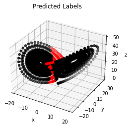
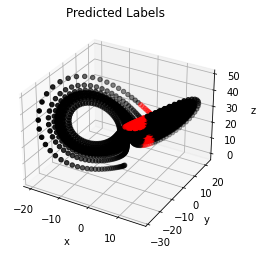
The Fig. 8 illustrates the performance of neural network models in mismatched condition. The initial conditions for training data are sampled according to Eq. (2a) and for validation data are sampled according to Eq. (3b). In this example, the neural network models almost completely miss the region of unstable data points and fail to identify them reliably. This is also reflected in the low precision and recall values of and respectively. As a reference, the Fig. 9 shows the result on the same validation set as Fig. 8 using a neural network model that has the initial conditions for training data sampled according to Eq. 2b. A comparison of Fig. 8 and Fig. 9, shows the importance of initial conditions on the performance of neural networks for the specific task of identification of unstable data points of Lorenz system. One can clearly see that using the features described in Section V as-is, limits the usability of the neural network models, in that, the models cannot be used for the mismatched scenario.
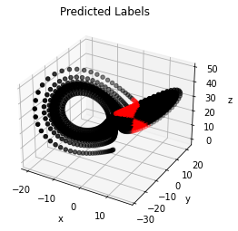
Neural network models that are generalizable should be able to perform reliably on a broad variety of validation data. To this end, we train neural network models that have the initial conditions for the training data sampled from a slightly larger interval. Specifically, we use Eq. (2c) to sample the initial conditions for training data. The Fig. 10 shows the classification result when the initial conditions for training data were sampled according to Eq. (2c) and for validation data were sampled according to Eq. (3b). The precision and recall values are and respectively. Again, the low recall score indicates a high number of false negatives (which is also reflected as less number of data points labelled in red in Fig. 10). Although the classification results of the models shown in Fig. 10 are not comparable to matched case shown in Fig. 9, these models are able to capture the region of unstable data points better than those in Fig. 8. Since it is impractical to have a matched model for every validation set (one whose initial conditions during training have been sampled from the same interval, such as the one shown in Fig. 9), we think that model trained according to Eq. (2c) (such as the one shown in Fig. 10) might serve as a good candidate for training neural networks that can perform reliably on a wide variety of validation data. In the section VII, we show how the normalization scheme helps in further improving the performance of models trained according to Eq. (2c) in mismatched conditions.


VII Normalization
In order to understand why the classification results shown in Fig. 8 are worse than those in Fig. 9, we look at the statistics of the training and validation data. The Fig. 11 compares the histograms and kernel density estimates of the features of training and validation data in the mismatched and matched cases. For simplicity, only the x-coordinate features are shown. In the Fig. 11(a), the initial conditions of training data were sampled according to Eq. (2a) and those of the validation data were sampled according to Eq. (3b). One can notice that there is a strong mismatch between the histograms and kernel density estimates of training and validation data in Fig. 11(a). This mismatch leads to a degradation in the performance of the neural networks. In contrast, the initial conditions of the training data were sampled according to Eq. (2b) in Fig. 11(b). The initial conditions for validation data were sampled according to Eq. (3b). Since the initial conditions for training and validation data were sampled from the same interval in Fig. 11(b), there is no mismatch between their histograms and the kernel density estimates. Consequently, the performance of neural network models trained on this data is better, as evidenced by higher precision and recall scores.
In this work, we employ a normalization scheme that reduces the mismatch between training and validation data. Intuitively, we think that lesser the mismatch between the distributions of training and validation data, better will be the performance. With such a normalization scheme, the initial conditions for the training data can be sampled from a relatively small interval and the trained neural network models will give reliable performance on different kinds of validation data.
As described in section IV, we use Lorenz systems for training the neural network. We sample the initial conditions of training data according to Eq. (2c), as we think this interval is a good candidate for training generalizable models. We normalize each of the Lorenz systems separately. As noted in section V, the input to the neural network is a dimensional feature vector. We calculate the mean and standard deviation along each of the feature dimensions for each of the Lorenz Systems. Specifically, if represents x-coordinate of one of the data points of the Lorenz system, we transform according to Eq. 5a, where the mean and standard deviation are given by Eq. (5b) and Eq. (5c) respectively.
| (5a) |
| (5b) |
| (5c) |
We perform normalization for both training and validation data. The Fig. 12 compares the histograms and kernel density estimates of the training and validation data before and after normalization. One can clearly see that after normalization (Fig. 12(b)), the histograms and kernel density estimates of training and validation data have a greater overlap and a reduced mismatch.


The Fig. 13 shows the location of stable and unstable data points before and after normalization. Thus, we are able to verify that the normalization scheme does not alter the relative location of stable and unstable data points. It merely shifts the data points along the axes.


VII.1 Results
The Fig. 14 shows the classification result in the mismatched case when the neural network is trained on normalized feature vectors. The initial condition for training are sampled according to Eq. 2c and those for validation are sampled according to Eq. 3b. The precision are recall scores are and respectively. One can also see that the results of Fig. 14 clearly outperform those of Fig. 8, Fig. 9 and Fig. 10. This also highlights that neural network models are sensitive to the mismatch between distributions of training and validation data and that normalization schemes are necessary to reduce the mismatch.
We also verify whether neural networks trained on normalized data , whose initial conditions are sampled according to Eq. (2c) can perform reliably on a wide variety of validation data. To this end, we test the neural network model on validation data whose initial conditions are sampled according to Eq. (3d), Eq. (3e) and Eq. (3f). The Fig. 15 shows the result of applying neural network models when the initial conditions of validation data were sampled according to Eq. (3d). This interval is completely outside of the interval used for sampling the initial conditions of training data (Eq. (2c)). Yet, we see that the classification performance is reasonably good, with a precision score of and a recall score of . The Fig. 16 and Fig. 17 show the classification performance when the initial conditions for validation data were sampled according to Eq. (3e) and Eq. (3f) respectively. Both these intervals are much wider compared to those for sampling initial conditions for training data (Eq. (2c)). Again, we see that the performance of neural network models is reasonably accurate. The precision and recall scores of the classification result shown in Fig. 16 are and respectively. The precision and recall scores of the classification result shown in Fig. 17 are and respectively.
The Tables 1 and 2 summarize the results of our experiments by depicting the average precision and recall scores without and with normalization respectively. For each row, neural network models are trained using training data whose initial conditions are sampled from the intervals specified in the first column. As described in Section IV, we use 25 Lorenz systems for training and 5 Lorenz systems for validation. The mean precision and recall values are obtained by averaging over the 5 validation lorenz systems. We also show the standard deviation to quantify how much the precision and recall scores deviate from the mean. Per Table 1, we observe that the performance of the neural network models drop significantly in the mismatched case (Rows and of Table 1). We choose the interval to sample initial conditions for training data for our further experiments, per our observation that it represents a valid subset of the validation data intervals that the neural network is likely to encounter. The results in Table 2 indicate that our assumption is justified. The neural networks whose training data are sampled from the interval perform well on a wide variety of validation datasets. These results also show that our normalization scheme greatly helps in improving the performance of neural networks on mismatched data and is a promising step towards training generalizable neural networks for this classification task.
| Training | Validation | Mean Precision | Mean Recall | Stddev-Precision | Stddev-Recall |
|---|---|---|---|---|---|
| Training | Interval | Mean Precision | Mean Recall | Stddev-Precision | Stddev-Recall |
|---|---|---|---|---|---|
| sample | to sample | ||||
| from | ics for Validation | ||||


VIII Conclusions
In this paper, we explore the use of neural networks to classify the discrete states of a Lorenz system. Such systems are highly sensitive to the initial conditions and identifying the location of stable and unstable states is a challenging task.Our numeral results suggest that classification performed using a feed forward neural network model can accommodate sensitivity to initial conditions in the training and validation data sets. The classification performance degrades when there is a mismatch between initial conditions used for generating training and validation data sets. We introduce a normalization scheme and show that it significantly improves the classification performance of neural network models in mismatched conditions. More broadly, our results show the feasibility of using neural networks to study stability aspects of chaotic systems like Lorenz63 systems. Improvement in state estimation via neural network based classification can significantly enhance automated decision making in complex systems within an SDM context. Future work will explore the scalability and explainability aspects of our normalization scheme within neural network based classification applied to large scale complex system state estimation.
Acknowledgements.
The research described in this paper is supported by the Mathematics of Artificial Reasoning in Science (MARS) Initiative at Pacific Northwest National Laboratory (PNNL). It was conducted under the Laboratory Directed Research and Development Program at PNNL, a multiprogram national laboratory operated by Battelle for the U.S. Department of Energy under DE-AC05-76RL01830.References
- Amiri, Shirazi, and Zhang (2019) S. Amiri, M. S. Shirazi, and S. Zhang, “Robot sequential decision making using lstm-based learning and logical-probabilistic reasoning,” CoRR (2019).
- Sutton and Barto (2018) R. S. Sutton and A. G. Barto, Reinforcement learning: An introduction (MIT press, 2018).
- He et al. (2015) K. He, X. Zhang, S. Ren, and J. Sun, “Deep residual learning for image recognition,” (2015), arXiv:1512.03385 [cs.CV] .
- Hinton et al. (2012) G. Hinton, L. Deng, D. Yu, G. E. Dahl, A. Mohamed, N. Jaitly, A. Senior, V. Vanhoucke, P. Nguyen, T. N. Sainath, and B. Kingsbury, “Deep neural networks for acoustic modeling in speech recognition: The shared views of four research groups,” IEEE Signal Processing Magazine 29, 82–97 (2012).
- Vaswani et al. (2017) A. Vaswani, N. Shazeer, N. Parmar, J. Uszkoreit, L. Jones, A. N. Gomez, L. u. Kaiser, and I. Polosukhin, “Attention is all you need,” in Advances in Neural Information Processing Systems, Vol. 30, edited by I. Guyon, U. V. Luxburg, S. Bengio, H. Wallach, R. Fergus, S. Vishwanathan, and R. Garnett (Curran Associates, Inc., 2017) pp. 5998–6008.
- (6) A. W. Senior, R. Evans, J. Jumper, J. Kirkpatrick, L. Sifre, T. Green, C. Qin, A. Žídek, A. W. R. Nelson, A. Bridgland, H. Penedones, S. Petersen, K. Simonyan, S. Crossan, P. Kohli, D. T. Jones, D. Silver, K. Kavukcuoglu, and D. Hassabis, “Improved protein structure prediction using potentials from deep learning,” Nature. 577.
- (7) K. Narendra and K. Parthasarathy, “Identification and control of dynamical systems using neural networks,” IEEE transactions on neural networks 1.
- Lellep et al. (2020) M. Lellep, J. Prexl, M. Linkmann, and B. Eckhardt, “Using machine learning to predict extreme events in the hénon map,” Chaos: An Interdisciplinary Journal of Nonlinear Science 30, 013113 (2020).
- Hochreiter and Schmidhuber (1997) S. Hochreiter and J. Schmidhuber, “Long short-term memory,” Neural computation 9, 1735–1780 (1997).
- (10) P. R. Vlachas, W. Byeon, Z. Y. Wan, T. P. Sapsis, and P. Koumoutsakos, “Data-driven forecasting of high-dimensional chaotic systems with long short-term memory networks,” Proceedings. 474.
- Chattopadhyay, Hassanzadeh, and Subramanian (2020) A. Chattopadhyay, P. Hassanzadeh, and D. Subramanian, “Data-driven predictions of a multiscale lorenz 96 chaotic system using machine-learning methods: reservoir computing, artificial neural network, and long short-term memory network,” Nonlinear Processes in Geophysics 27, 373–389 (2020).
- Pathak et al. (2018a) J. Pathak, A. Wikner, R. Fussell, S. Chandra, B. R. Hunt, M. Girvan, and E. Ott, “Hybrid forecasting of chaotic processes: Using machine learning in conjunction with a knowledge-based model,” CoRR abs/1803.04779 (2018a), arXiv:1803.04779 .
- Pathak et al. (2018b) J. Pathak, B. Hunt, M. Girvan, Z. Lu, and E. Ott, “Model-free prediction of large spatiotemporally chaotic systems from data: A reservoir computing approach,” Phys. Rev. Lett. 120, 024102 (2018b).
- Champion et al. (2019) K. Champion, B. Lusch, J. N. Kutz, and S. L. Brunton, “Data-driven discovery of coordinates and governing equations,” Proceedings of the National Academy of Sciences 116, 22445–22451 (2019).
- Brugnago et al. (2020) E. L. Brugnago, T. A. Hild, D. Weingärtner, and M. W. Beims, “Classification strategies in machine learning techniques predicting regime changes and durations in the lorenz system,” Chaos: An Interdisciplinary Journal of Nonlinear Science 30, 053101 (2020).
- Sugiyama and Kawanabe (2012) M. Sugiyama and M. Kawanabe, Machine learning in non-stationary environments: Introduction to covariate shift adaptation (MIT press, 2012).
- Vincent et al. (2017) E. Vincent, S. Watanabe, A. A. Nugraha, J. Barker, and R. Marxer, “An analysis of environment, microphone and data simulation mismatches in robust speech recognition,” Computer Speech I& Language 46, 535 – 557 (2017).
- Lai et al. (2019) G. Lai, B. Oguz, Y. Yang, and V. Stoyanov, “Bridging the domain gap in cross-lingual document classification,” (2019), arXiv:1909.07009 [cs.CL] .
- Scher and Messori (2019) S. Scher and G. Messori, “Generalization properties of feed-forward neural networks trained on lorenz systems,” Nonlinear processes in geophysics 26, 381–399 (2019).
- Lorenz (1963) E. N. Lorenz, “Deterministic nonperiodic flow journal of the atmospheric sciences vol. 20,” No. In. XX (1963).
- Ahnert et al. (2011) K. Ahnert, M. Mulansky, T. E. Simos, G. Psihoyios, C. Tsitouras, and Z. Anastassi, “Odeint – solving ordinary differential equations in c++,” (2011), 10.1063/1.3637934.
- Virtanen et al. (2020) P. Virtanen, R. Gommers, T. E. Oliphant, M. Haberland, T. Reddy, D. Cournapeau, E. Burovski, P. Peterson, W. Weckesser, J. Bright, S. J. van der Walt, M. Brett, J. Wilson, K. J. Millman, N. Mayorov, A. R. J. Nelson, E. Jones, R. Kern, E. Larson, C. J. Carey, İ. Polat, Y. Feng, E. W. Moore, J. VanderPlas, D. Laxalde, J. Perktold, R. Cimrman, I. Henriksen, E. A. Quintero, C. R. Harris, A. M. Archibald, A. H. Ribeiro, F. Pedregosa, P. van Mulbregt, and SciPy 1.0 Contributors, “SciPy 1.0: Fundamental Algorithms for Scientific Computing in Python,” Nature Methods 17, 261–272 (2020).
- Kingma and Ba (2017) D. P. Kingma and J. Ba, “Adam: A method for stochastic optimization,” (2017), arXiv:1412.6980 [cs.LG] .
- Chollet et al. (2015) F. Chollet et al., “Keras,” (2015).