This paper was converted on www.awesomepapers.org from LaTeX by an anonymous user.
Want to know more? Visit the Converter page.

Lorentz-covariant spinor wave packet

Kin-ya Oda and Juntaro Wada E-mail: [email protected]E-mail: [email protected]
Abstract

We propose a novel formulation for a manifestly Lorentz-covariant spinor wave-packet basis. The traditional definition of the spinor wave packet is problematic due to its unavoidable mixing with other wave packets under Lorentz transformations. Our approach resolves this inherent mixing issue. The wave packet we develop constitutes a complete set, enabling the expansion of a free spinor field while maintaining Lorentz covariance. Additionally, we present a Lorentz-invariant expression for zero-point energy.

Department of Mathematics, Tokyo Woman’s Christian University, Tokyo 167-8585, Japan
Department of Physics, University of Tokyo, Tokyo 113-0033, Japan

1 Introduction

In quantum mechanics, wave packets serve as a crucial conceptual and mathematical foundation. In real observations, we never encounter idealized plane-wave states, characterized by zero uncertainty in momentum and infinite uncertainty in position. They do not belong to the Hilbert space because of its non-normalizability. In quantum field theory (QFT), the plane-wave SS-matrix is traditionally used, but this approach results in divergences due to the squared energy-momentum delta function. This makes the plane-wave SS-matrix computation more of a mnemonic than a rigorous derivation for observables; see e.g. Ref. [1].

Wave packet states have been extensively discussed in various contexts of particle physics phenomenology, including anomalies in vector meson decay [2], corrections to Fermi’s golden rule [3, 4], searches for dark photons [5], applications in quantum computation [6, 7, 8], and studies of neutrino oscillation [9, 10, 11, 12, 13, 14, 15, 16, 17, 18, 19, 20].

Despite these applications, theoretical efforts to construct QFT based on wave-packet states have been limited. Previous work has employed Gaussian formalism, utilizing Gaussian wave functions as a complete basis for expanding the free one-particle Hilbert space. This approach has revealed phenomena like time-boundary effects, which are unobservable in plane-wave formalism [21]. However, the Gaussian formalism breaks manifest Lorentz covariance, necessitating a refinement for both aesthetic and pragmatic reasons.

The absence of manifest Lorentz covariance is unsatisfying, as historically, physics has advanced through symmetry-based formalisms, such as the Dirac [22] and Becchi-Rouet-Stora-Tyutin (BRST) [23, 24, 25] formalisms. Therefore, it is desirable to develop a manifestly Lorentz-covariant wave packet formalism.

Practically, the Gaussian formalism complicates calculations due to the lack of Lorentz covariance, evident in the difficulty of deriving explicit analytic formulas for Gaussian wave functions in position space. In contrast, our previous study demonstrated the expansion of scalar fields in QFT using a complete basis of Lorentz-invariant wave packets, facilitating the derivation of analytic formulas for Lorentz-invariant wave functions in scalar fields [26]. Also, the Gaussian wave packet is shown to be a non-relativistic limit of the Lorentz-invariant wave packet for the scalar fields [26].

In this study, we investigate the wave packet basis for spinors within a Lorentz-covariant framework. Traditional methodologies, including Gaussian formalism (refer to Appendix A in Ref. [27] for an overview) and other approaches towards Lorentz-covariant spinor wave packets [28, 29, 30, 31, 32], assume that the spin dependence of spinor wave packets aligns with that of plane waves. However, this assumption introduces a significant complication: it leads to a complex Lorentz transformation law, which unexpectedly intertwines wave-packet states with different central momenta and positions. Such a phenomenon is physically paradoxical. Imagine a scenario where a single particle is depicted by a wave packet with a distinct central momentum and position. The blending of this wave packet with others having varying central momenta and positions effectively results in an unphysical merging of distinct particles under Lorentz transformation, which is a challenging notion for conventional theories.

In response to this issue, this paper introduces a novel definition of the spinor wave packet that circumvents this problematic mixing: |X,P,S;σ\rrangle\left\lvert X,P,S;\sigma\right\rrangle, where XX and PP are its position and momentum centers, SS its spin, and σ\sigma its spatial width-squared. The wave packet |X,P,S;σ\rrangle\left\lvert X,P,S;\sigma\right\rrangle is defined by

\llanglep,s|X,P,S;σ\rrangle\displaystyle\left\llangle p,s\mathchoice{\;}{\;}{\,}{\,}\middle|\mathchoice{\;}{\;}{\,}{\,}X,P,S;\sigma\right\rrangle eip(X+iσP)u¯(p,s)u(P,S)\displaystyle\propto e^{-ip\cdot\left(X+i\sigma P\right)}\overline{u}\!\left(p,s\right)u\!\left(P,S\right)
=eip(X+iσP)v¯(P,S)v(p,s),\displaystyle\quad=-e^{-ip\cdot\left(X+i\sigma P\right)}\overline{v}\!\left(P,S\right)v\!\left(p,s\right), (1)

where |p,s\rrangle\left\lvert p,s\right\rrangle is a Lorentz-friendly plane-wave basis state with the momentum pp and spin ss; further details will be given in subsequent sections, especially in Eq. (34).

Our definition ensures that wave packets remain separate and distinct under Lorentz transformations. We then establish the completeness of this newly defined spinor wave packet within the free one-particle subspace. Expanding on this concept, we demonstrate that the spinor field can be effectively expanded using our spinor wave packet. Additionally, we explore the application of this approach to several well-established operators in the wave packet basis, providing a comprehensive understanding of its implications in quantum field theory.

The paper is organized as follows: Section 2 introduces the new Lorentz-covariant spinor wave-packet basis in the one-particle subspace. Section 3 extends this to the creation and annihilation operators, showing how the free fermion field can be expanded using this basis. Finally, Section 4 presents the expression of several QFT operators in terms of wave packets.

2 Lorentz-covariant spinor wave packet

In this section, we point out that the known representation of a spinor wave packet suffers from mixing with other wave packets under Lorentz transformations, and propose a complete set of Lorentz-covariant spinor wave-packet basis without the difficulty of mixing.

We work in the (d+1)\left(d+1\right)-dimensional Minkowski space 𝐌d+1\mathbf{M}^{d+1} spanned by coordinate system x=(x0,𝒙)=(x0,x1,,xd)1,dx=\left(x^{0},\boldsymbol{x}\right)=\left(x^{0},x^{1},\dots,x^{d}\right)\in\mathbb{R}^{1,d}, with d=3d=3 spatial dimensions. We take the almost-plus metric signature (,+,,+)\left(-,+,\dots,+\right); expressions in the opposite convention can be found in Appendix D. We only consider a massive field, m>0m>0, and always take (d+1)\left(d+1\right)-momenta on-shell, p0=m2+𝒑2p^{0}=\sqrt{m^{2}+\boldsymbol{p}^{2}}, throughout this paper unless otherwise stated. When an on-shell momentum appears in an argument of a function such as f(𝒑)f\!\left(\boldsymbol{p}\right), we use both dd and (d+1)\left(d+1\right)-dimensional notations interchangeably: f(𝒑)=f(p)f\!\left(\boldsymbol{p}\right)=f\!\left(p\right).

2.1 Spinor plane waves, revisited

To spell out our notation, we summarize basic known facts on the spinor plane waves. A free Dirac field ψ^(x)\widehat{\psi}\!\left(x\right) can be expanded by plane wave as follows,

ψ^(x)\displaystyle\widehat{\psi}\!\left(x\right) =sdd𝒑2p0(u(p,s)eipx(2π)d/2α^(p,s)+v(p,s)eipx(2π)d/2β^(p,s)),\displaystyle=\sum_{s}\int{\text{d}^{d}\boldsymbol{p}\over 2p^{0}}\left(u(p,s){e^{ip\cdot x}\over\left(2\pi\right)^{d/2}}\widehat{\alpha}\!\left(p,s\right)+v(p,s){e^{-ip\cdot x}\over\left(2\pi\right)^{d/2}}\widehat{\beta}^{\dagger}\!\left(p,s\right)\right), (2)

where u(p,s)u\!\left(p,s\right) and v(p,s)v\!\left(p,s\right) are plane-wave solutions of the Dirac equation

(i+m)u(p,s)=0,\displaystyle(i\not{p}+m)u(p,s)=0,
(im)v(p,s)=0,\displaystyle(i\not{p}-m)v(p,s)=0, (3)

with s=±1/2s=\pm 1/2 being the spin in the rest frame of each solution. Throughout this paper, we suppress the spinor indices a=1,,2(d+1)/2a=1,\dots,2^{\left\lfloor\left(d+1\right)/2\right\rfloor} for ψ^\widehat{\psi}, uu, vv, etc. when unnecessary.

These solutions satisfy the following completeness relations,

su(p,s)u¯(p,s)\displaystyle\sum_{s}u(p,s)\overline{u}(p,s) =i+m,\displaystyle=-i\not{p}+m,
sv(p,s)v¯(p,s)\displaystyle\sum_{s}v(p,s)\overline{v}(p,s) =im,\displaystyle=-i\not{p}-m, (4)

and their normalization is

u¯(p,s)u(p,s)=2mδss,\displaystyle\overline{u}(p,s)u\!\left(p,s^{\prime}\right)=2m\delta_{ss^{\prime}},
v¯(p,s)v(p,s)=2mδss,\displaystyle\overline{v}(p,s)v\!\left(p,s^{\prime}\right)=-2m\delta_{ss^{\prime}}, (5)

where ψ¯:=ψβ\overline{\psi}:=\psi^{\dagger}\beta is the Dirac adjoint.111 We adopt the spinor notation in Ref. [1]: {γμ,γν}=2ημνI\left\{\gamma^{\mu}\,,\>\gamma^{\nu}\right\}=2\eta^{\mu\nu}I, where η:=diag(1,1,,1)\eta:=\operatorname{diag}\!\left(-1,1,\dots,1\right) and II is the unit matrix in the spinor space. Here, β:=iγ0\beta:=i\gamma^{0} is distinguished from the operator β^\widehat{\beta}. The coefficients α^(p,s)\widehat{\alpha}\!\left(p,s\right) and β^(p,s)\widehat{\beta}^{\dagger}\!\left(p,s\right) in Eq. (2) are the annihilation and creation operators for particle and anti-particle, respectively, that satisfy the following anticommutation relations:

{α^(p,s),α^(p,s)}\displaystyle\left\{\widehat{\alpha}\!\left(p,s\right)\,,\>\widehat{\alpha}^{\dagger}\!\left(p^{\prime},s^{\prime}\right)\right\} =δss2p0δd(𝒑𝒑)1^,\displaystyle=\delta_{ss^{\prime}}2p^{0}\delta^{d}\!\left(\boldsymbol{p}-\boldsymbol{p}^{\prime}\right)\widehat{1},
{β^(p,s),β^(p,s)}\displaystyle\left\{\widehat{\beta}\!\left(p,s\right)\,,\>\widehat{\beta}^{\dagger}\!\left(p^{\prime},s^{\prime}\right)\right\} =δss2p0δd(𝒑𝒑)1^,\displaystyle=\delta_{ss^{\prime}}2p^{0}\delta^{d}\!\left(\boldsymbol{p}-\boldsymbol{p}^{\prime}\right)\widehat{1},
others =0.\displaystyle=0. (6)

Free one-particle subspaces of particle and anti-particle are spanned by the following plane-wave bases:

α^(p,s)|0\displaystyle\widehat{\alpha}^{\dagger}\!\left(p,s\right)\ket{0} =:|p,s,n\rrangle,\displaystyle=:\left\lvert p,s,n\right\rrangle, β^(p,s)|0\displaystyle\widehat{\beta}^{\dagger}\!\left(p,s\right)\ket{0} =:|p,s,nc\rrangle,\displaystyle=:\left\lvert p,s,n^{\text{c}}\right\rrangle, (7)

where nn and ncn^{\text{c}} denote the particle and anti-particle of the species nn, respectively. The anticommutator (6) leads to the inner product:

\llanglep,s,N|p,s,N\rrangle\displaystyle\left\llangle p,s,N\mathchoice{\;}{\;}{\,}{\,}\middle|\mathchoice{\;}{\;}{\,}{\,}p^{\prime},s^{\prime},N^{\prime}\right\rrangle :=2p0δd(𝒑𝒑)δssδNN,\displaystyle:=2p^{0}\delta^{d}\!\left(\boldsymbol{p}-\boldsymbol{p}^{\prime}\right)\delta_{ss^{\prime}}\delta_{NN^{\prime}}, (8)

where N=n,ncN=n,n^{\text{c}} labels the particle and anti-particle. The normalization (8) leads to the completeness relation (resolution of identity) in the free one-particle subspace of each N=n,ncN=n,n^{\text{c}}:

sdd𝒑2p0|p,s,N\rrangle\llanglep,s,N|\displaystyle\sum_{s}\int{\text{d}^{d}\boldsymbol{p}\over 2p^{0}}\left\lvert p,s,N\right\rrangle\left\llangle p,s,N\right\rvert =1^.\displaystyle=\hat{1}. (9)

The Lorentz transformation law of the plane wave reads

U^(Λ)|p,s\rrangle=s|Λp,s\rrangleDss(W(Λ,p)),\displaystyle\widehat{U}\!\left(\Lambda\right)\left\lvert p,s\right\rrangle=\sum_{s^{\prime}}\left\lvert\Lambda p,s^{\prime}\right\rrangle D_{s^{\prime}s}\bigl{(}{W\!\left(\Lambda,p\right)}\bigr{)}, (10)

where DD is the spin-ss representation of the Winger rotation SO(d)SO(d); see Appendix B for details.

2.2 Lorentz-covariant spinor wave packet

In this subsection, we first briefly review basic facts on Lorentz-invariant scalar wave packets [33, 34], which is discussed in our previous work [26]. Next, we point out the difficulty in the conventional treatment of the spinor wave packet [28, 29, 30, 31]. Then, we propose a new definition of the spinor wave packet and show that we can avoid this difficulty in our expression.

2.2.1 Brief review of Lorentz-invariant scalar wave packet

For central position XX and momentum PP in (d+1)\left(d+1\right)-dimensions, a Lorentz-invariant scalar wave packet |Π\rrangle\left\lvert\Pi\right\rrangle is defined by [33, 34]:222See e.g. Refs. [30, 26] for reviews.

\llanglep|Π\rrangle\displaystyle\left\llangle p\mathchoice{\;}{\;}{\,}{\,}\middle|\mathchoice{\;}{\;}{\,}{\,}\Pi\right\rrangle :=Nϕeip(X+iσP),\displaystyle:=N_{\phi}e^{-ip\cdot\left(X+i\sigma P\right)}, (11)

where Π\Pi denotes the phase space333 Here, Π\Pi includes the wave-packet central time X0X^{0}. Though P0=m2+𝑷2P^{0}=\sqrt{m^{2}+\boldsymbol{P}^{2}} is not an independent variable, we also include it for the convenience of writing its Lorentz transformation below.

Π\displaystyle\Pi :=(X,P),\displaystyle:=\left(X,P\right), (12)

and the normalization factor

Nϕ\displaystyle N_{\phi} :=(σπ)d14Kd12(2σm2)\displaystyle:={\left(\sigma\over\pi\right)^{d-1\over 4}\over\sqrt{K_{d-1\over 2}\!\left(2\sigma m^{2}\right)}} (13)

provides \llangleΠ|Π\rrangle=1\left\llangle\Pi|\Pi\right\rrangle=1, in which Kn(z)K_{n}\!\left(z\right) is the modified Bessel function of the second kind. Here and hereafter, we fix σ\sigma unless otherwise stated.

The wave function and the inner product are obtained as [33, 26]

\llanglex|Π\rrangle\displaystyle\left\llangle x\mathchoice{\;}{\;}{\,}{\,}\middle|\mathchoice{\;}{\;}{\,}{\,}\Pi\right\rrangle =Nϕmd12πKd12(ξ)ξd12,\displaystyle=N_{\phi}{m^{d-1}\over\sqrt{2\pi}}{K_{d-1\over 2}\!\left(\left\|\xi\right\|\right)\over\left\|\xi\right\|^{d-1\over 2}}, (14)
\llangleΠ|Π\rrangle\displaystyle\left\llangle\Pi\mathchoice{\;}{\;}{\,}{\,}\middle|\mathchoice{\;}{\;}{\,}{\,}\Pi^{\prime}\right\rrangle =Nϕ2(2πm2)d12Kd12(Ξ)Ξd12,\displaystyle=N_{\phi}^{2}\left(2\pi m^{2}\right)^{d-1\over 2}{K_{d-1\over 2}\left(\left\|\Xi\right\|\right)\over\left\|\Xi\right\|^{d-1\over 2}}, (15)

where for any complex vector VμV^{\mu}, we write V:=V2\left\|V\right\|:=\sqrt{-V^{2}}, namely,

ξ\displaystyle\left\|\xi\right\| =mσ2m2+(xX)22iσP(xX),\displaystyle=m\sqrt{\sigma^{2}m^{2}+\left(x-X\right)^{2}-2i\sigma P\cdot\left(x-X\right)}, (16)
Ξ\displaystyle\left\|\Xi\right\| =m((XX)iσ(P+P))2,\displaystyle=m\sqrt{\bigl{(}\left(X-X^{\prime}\right)-i\sigma\left(P+P^{\prime}\right)\bigr{)}^{2}}, (17)

with ξμ:=m[σPμ+i(xX)μ]\xi^{\mu}:=m\left[\sigma P^{\mu}+i\left(x-X\right)^{\mu}\right] and Ξμ:=m[σ(P+P)μ+i(XX)μ]\Xi^{\mu}:=m\left[\sigma\left(P+P^{\prime}\right)^{\mu}+i\left(X-X^{\prime}\right)^{\mu}\right].444 The abuse of notation is understood such that a vector-squared V2:=(V0)2+𝑽2V^{2}:=-\left(V^{0}\right)^{2}+\boldsymbol{V}^{2} is distinguished from the second component of VV by the context. We note that there is no branch-cut ambiguity for the square root as long as m>0m>0  [26].

With this state, the momentum expectation value and its (co)variance become [33]

\llanglep^μ\rrangleϕ\displaystyle\left\llangle\hat{p}^{\mu}\right\rrangle_{\phi} :=dd𝒑2p0\llangleΠ|p\rranglepμ\llanglep|Π\rrangle=ϕPμ,\displaystyle:=\int{\text{d}^{d}\boldsymbol{p}\over 2p^{0}}\left\llangle\Pi\mathchoice{\;}{\;}{\,}{\,}\middle|\mathchoice{\;}{\;}{\,}{\,}p\right\rrangle p^{\mu}\left\llangle p\mathchoice{\;}{\;}{\,}{\,}\middle|\mathchoice{\;}{\;}{\,}{\,}\Pi\right\rrangle=\mathcal{M}_{\phi}P^{\mu}, (18)
\llanglep^μp^ν\rrangleϕ\displaystyle\left\llangle\hat{p}^{\mu}\hat{p}^{\nu}\right\rrangle_{\phi} =Kd+32(2σm2)Kd12(2σm2)PμPν+ϕ2σημν,\displaystyle={K_{d+3\over 2}\!\left(2\sigma m^{2}\right)\over K_{d-1\over 2}\!\left(2\sigma m^{2}\right)}P^{\mu}P^{\nu}+{\mathcal{M}_{\phi}\over 2\sigma}\eta^{\mu\nu}, (19)

where

ϕ\displaystyle\mathcal{M}_{\phi} :=Kd+12(2σm2)Kd12(2σm2).\displaystyle:={K_{d+1\over 2}\!\left(2\sigma m^{2}\right)\over K_{d-1\over 2}\!\left(2\sigma m^{2}\right)}. (20)

In general, a matrix element of p^\hat{p} becomes

\llanglep^μ\rrangleΠ,Π\displaystyle\left\llangle\hat{p}^{\mu}\right\rrangle_{\Pi,\Pi^{\prime}} :=dd𝒑2p0\llangleΠ|p\rranglepμ\llanglep|Π\rrangle=(2πm2)d12Nϕ2mΞμKd+12(Ξ)Ξd+12.\displaystyle:=\int{\text{d}^{d}\boldsymbol{p}\over 2p^{0}}\left\llangle\Pi\mathchoice{\;}{\;}{\,}{\,}\middle|\mathchoice{\;}{\;}{\,}{\,}p\right\rrangle p^{\mu}\left\llangle p\mathchoice{\;}{\;}{\,}{\,}\middle|\mathchoice{\;}{\;}{\,}{\,}\Pi^{\prime}\right\rrangle=\left(2\pi m^{2}\right)^{d-1\over 2}N_{\phi}^{2}\,m\Xi^{\mu}{K_{d+1\over 2}\!\left(\left\|\Xi\right\|\right)\over\left\|\Xi\right\|^{d+1\over 2}}. (21)

Let us consider a spacelike hyperplane ΣN,T={X|NX+T=0}\Sigma_{N,T}=\Set{X}{N\cdot X+T=0} in the space of central position XX; see Appendix A. One can write the completeness relation in the position-momentum phase space in a manifestly Lorentz-invariant fashion [26] (see also Ref. [33]):

d2dΠϕ|Π\rrangle\llangleΠ|\displaystyle\int\text{d}^{2d}\Pi_{\phi}\left\lvert\Pi\right\rrangle\left\llangle\Pi\right\rvert =1^,\displaystyle=\hat{1}, (22)

where 1^\hat{1} denotes the identity operator in the one-particle subspace and the Lorentz-invariant phase-space volume element is given by

d2dΠϕ\displaystyle\int\text{d}^{2d}\Pi_{\phi} :=1ϕddΣXμ(2π)d(2Pμ)dd𝑷2P0,\displaystyle:={1\over\mathcal{M}_{\phi}}\int{\text{d}^{d}\Sigma^{\mu}_{X}\over\left(2\pi\right)^{d}}\left(-2P_{\mu}\right){\text{d}^{d}\boldsymbol{P}\over 2P^{0}}, (23)

in which

ddΣXμ\displaystyle\text{d}^{d}\Sigma^{\mu}_{X} :=dd+1Xδ(NX+T)Nμ\displaystyle:=\text{d}^{d+1}X\,\delta\!\left(N\cdot X+T\right)N^{\mu} (24)

is the Lorentz-covariant volume element. We stress that σ\sigma is not summed nor integrated in the identity (22) and that the identity holds for any fixed σ\sigma.

Let us consider a “time-slice frame” Xˇ\check{X} of the central-position space in which ΣˇNˇ,T\check{\Sigma}_{\check{N},T} becomes an equal-time hyperplane Xˇ0=T\check{X}^{0}=T,

Xˇ\displaystyle\check{X} :=1(N)X,\displaystyle:=\mathscr{L}^{-1}\!\left(N\right)X, (25)

where the “standard” Lorentz transformation (N)\mathscr{L}\!\left(N\right) is defined by N=:(N)N=:\mathscr{L}\!\left(N\right)\ell, with \ell denoting :=(1,𝟎)\ell:=\left(1,\boldsymbol{0}\right) in any frame; note that Nˇ=1(N)N=\check{N}=\mathscr{L}^{-1}\!\left(N\right)N=\ell by definition; see Appendix A for details. On the constant-Xˇ0\check{X}^{0} hyperplane ΣˇNˇ,T={Xˇ|Xˇ0=T}\check{\Sigma}_{\check{N},T}=\Set{\check{X}}{\check{X}^{0}=T}, the Lorentz-invariant phase-space volume element reduces to the familiar form:

d2dΠˇϕ\displaystyle\int\text{d}^{2d}\check{\Pi}_{\phi} =1ϕXˇ0=Tdd𝑿ˇdd𝑷ˇ(2π)d.\displaystyle={1\over\mathcal{M}_{\phi}}\int_{\check{X}^{0}=T}{\text{d}^{d}\boldsymbol{\check{X}}\,\text{d}^{d}\boldsymbol{\check{P}}\over\left(2\pi\right)^{d}}. (26)

Note that ϕ1\mathcal{M}_{\phi}\to 1 in the non-relativistic limit σm21\sigma m^{2}\gg 1.

2.2.2 Difficulty in spin-diagonal representation

In the literature [28, 29, 30, 31] a so to say spin-diagonal one-particle wave-packet state |Π,S\rrangleD\left\lvert\Pi,S\right\rrangle_{\text{D}} with a spin SS has been defined as

\llanglep,s|Π,S\rrangleD\displaystyle\left\llangle p,s\mathchoice{\;}{\;}{\,}{\,}\middle|\mathchoice{\;}{\;}{\,}{\,}\Pi,S\right\rrangle_{\text{D}} :=\llanglep|Π\rrangleδsS\displaystyle:=\left\llangle p\mathchoice{\;}{\;}{\,}{\,}\middle|\mathchoice{\;}{\;}{\,}{\,}\Pi\right\rrangle\delta_{sS} (27)

where \llanglep|Π\rrangle\left\llangle p\mathchoice{\;}{\;}{\,}{\,}\middle|\mathchoice{\;}{\;}{\,}{\,}\Pi\right\rrangle is nothing but the scalar Lorentz-invariant wave packet (11).555 In the literature, the normalization and XX-dependence [26] have been omitted. Its normalization becomes

\llangleΠ,S|Π,S\rrangleD\displaystyle\left\llangle\Pi,S\mathchoice{\;}{\;}{\,}{\,}\middle|\mathchoice{\;}{\;}{\,}{\,}\Pi^{\prime},S^{\prime}\right\rrangle_{\text{D}} =sdd𝒑2p0\llangleΠ,S|p,s\rrangleD\llanglep,s|Π,S\rrangleD\displaystyle=\sum_{s}\int{\text{d}^{d}\boldsymbol{p}\over 2p^{0}}\left\llangle\Pi,S\mathchoice{\;}{\;}{\,}{\,}\middle|\mathchoice{\;}{\;}{\,}{\,}p,s\right\rrangle_{\text{D}}\left\llangle p,s\mathchoice{\;}{\;}{\,}{\,}\middle|\mathchoice{\;}{\;}{\,}{\,}\Pi^{\prime},S^{\prime}\right\rrangle_{\text{D}}
=sdd𝒑2p0\llangleΠ|p\rrangle\llanglep|Π\rrangle\displaystyle=\sum_{s}\int{\text{d}^{d}\boldsymbol{p}\over 2p^{0}}\left\llangle\Pi\mathchoice{\;}{\;}{\,}{\,}\middle|\mathchoice{\;}{\;}{\,}{\,}p\right\rrangle\left\llangle p\mathchoice{\;}{\;}{\,}{\,}\middle|\mathchoice{\;}{\;}{\,}{\,}\Pi^{\prime}\right\rrangle
=\llangleΠ|Π\rrangleδSS,\displaystyle=\left\llangle\Pi\mathchoice{\;}{\;}{\,}{\,}\middle|\mathchoice{\;}{\;}{\,}{\,}\Pi^{\prime}\right\rrangle\delta_{SS^{\prime}}, (28)

where \llangleΠ|Π\rrangle\left\llangle\Pi\mathchoice{\;}{\;}{\,}{\,}\middle|\mathchoice{\;}{\;}{\,}{\,}\Pi^{\prime}\right\rrangle is given in Eq. (15).666 An inner product of the spin-diagonal wave-packet state and another state |ψ\Ket{\psi} is understood as \llangleΠ,S|ψD:=(|Π,S\rrangleD)|ψ=:\llangleΠ,S|D|ψ\left\llangle\Pi,S\mathchoice{\;}{\;}{\,}{\,}\middle|\mathchoice{\;}{\;}{\,}{\,}\psi\right\rangle_{\text{D}}:=\left(\left\lvert\Pi,S\right\rrangle_{\text{D}}\right)^{\dagger}\Ket{\psi}=:\left\llangle\Pi,S\right\rvert_{\text{D}}\Ket{\psi}. We will never consider an inner product of the spin-diagonal wave-packet state and a phase-space-diagonal wave-packet state that appears below so that this notation will not cause confusion. This leads to the following completeness relation in the one-particle subspace

Sd2dΠϕ|Π,S\rrangleD\llangleΠ,S|D\displaystyle\sum_{S}\int\text{d}^{2d}\Pi_{\phi}\left\lvert\Pi,S\right\rrangle_{\text{D}}\left\llangle\Pi,S\right\rvert_{\text{D}} =1^,\displaystyle=\hat{1}, (29)

generalizing the completeness relation of the scalar wave packet (22).

Once the wave-packet state is defined, its Lorentz transformation law is obtained as

U^(Λ)|Π,S\rrangleD\displaystyle\widehat{U}\!\left(\Lambda\right)\left\lvert\Pi,S\right\rrangle_{\text{D}} =sdd𝒑2p0U^(Λ)|p,s\rrangle\llanglep,s|Π,S\rrangleD\displaystyle=\sum_{s}\int{\text{d}^{d}\boldsymbol{p}\over 2p^{0}}\widehat{U}\!\left(\Lambda\right)\left\lvert p,s\right\rrangle\left\llangle p,s\mathchoice{\;}{\;}{\,}{\,}\middle|\mathchoice{\;}{\;}{\,}{\,}\Pi,S\right\rrangle_{\text{D}}
=s,sdd𝒑2p0Sd2dΠϕ|Π,S\rrangleD\llangleΠ,S|Λp,s\rrangleDDss(W(Λ,p))\llanglep,s|Π,S\rrangleD\displaystyle=\sum_{s,s^{\prime}}\int{\text{d}^{d}\boldsymbol{p}\over 2p^{0}}\sum_{S^{\prime}}\int\text{d}^{2d}\Pi^{\prime}_{\phi}\left\lvert\Pi^{\prime},S^{\prime}\right\rrangle_{\text{D}}\left\llangle\Pi^{\prime},S^{\prime}\mathchoice{\;}{\;}{\,}{\,}\middle|\mathchoice{\;}{\;}{\,}{\,}\Lambda p,s^{\prime}\right\rrangle_{\text{D}}D_{s^{\prime}s}\bigl{(}{W\!\left(\Lambda,p\right)}\bigr{)}\left\llangle p,s\mathchoice{\;}{\;}{\,}{\,}\middle|\mathchoice{\;}{\;}{\,}{\,}\Pi,S\right\rrangle_{\text{D}}
=Sd2dΠϕ|ΛΠ,S\rrangleD\llangleDSS(W(Λ,p^))\rrangleΠ,Π,\displaystyle=\sum_{S^{\prime}}\int\text{d}^{2d}\Pi^{\prime}_{\phi}\left\lvert\Lambda\Pi^{\prime},S^{\prime}\right\rrangle_{\text{D}}\left\llangle D_{S^{\prime}S}\bigl{(}{W\!\left(\Lambda,\hat{p}\right)}\bigr{)}\right\rrangle_{\Pi^{\prime},\Pi}, (30)

where

ΛΠ:=(ΛX,ΛP).\displaystyle\Lambda\Pi:=\left(\Lambda X,\Lambda P\right). (31)

and

\llangleDSS(W(Λ,p^))\rrangleΠ,Π:=\llangleΠ|(dd𝒑2p0DSS(W(Λ,p))|p\rrangle\llanglep|)|Π\rrangle.\displaystyle\left\llangle D_{S^{\prime}S}\bigl{(}{W\!\left(\Lambda,\hat{p}\right)}\bigr{)}\right\rrangle_{\Pi^{\prime},\Pi}:=\left\llangle\Pi^{\prime}\right\rvert\left(\int{\text{d}^{d}\boldsymbol{p}\over 2p^{0}}D_{S^{\prime}S}\bigl{(}{W\!\left(\Lambda,p\right)}\bigr{)}\left\lvert p\right\rrangle\left\llangle p\right\rvert\right)\left\lvert\Pi\right\rrangle. (32)

We see that the spin-diagonal choice (27) leads to the complicated transformation law (30) mixing the wave-packet state with the others having various centers of momentum and position.

Below, we will show that we can indeed realize a physically reasonable transformation law, so to say the phase-space-diagonal representation, which evades the mixing with other states (30):

U^(Λ)|Π,S\rrangle\displaystyle\widehat{U}\!\left(\Lambda\right)\left\lvert\Pi,S\right\rrangle =S|ΛΠ,S\rrangleCSS(Λ,Π),\displaystyle=\sum_{S^{\prime}}\left\lvert\Lambda\Pi,S^{\prime}\right\rrangle C_{S^{\prime}S}\!\left(\Lambda,\Pi\right), (33)

where CSS(Λ,Π)C_{S^{\prime}S}\!\left(\Lambda,\Pi\right) is a yet unspecified representation function.

2.2.3 Phase-space-diagonal representation

Instead of the conventional choice (27), we propose to define

\llanglep,s,N|Π,S,N\rrangle\displaystyle\left\llangle p,s,N\mathchoice{\;}{\;}{\,}{\,}\middle|\mathchoice{\;}{\;}{\,}{\,}\Pi,S,N^{\prime}\right\rrangle :=Nψeip(X+iσP)MsS(p,P)δNN\displaystyle:=N_{\psi}e^{-ip\cdot\left(X+i\sigma P\right)}M_{sS}\!\left(p,P\right)\delta_{NN^{\prime}}
(=NψNϕ\llanglep|Π\rrangleMsS(p,P)δNN),\displaystyle\left(={N_{\psi}\over N_{\phi}}\left\llangle p\mathchoice{\;}{\;}{\,}{\,}\middle|\mathchoice{\;}{\;}{\,}{\,}\Pi\right\rrangle M_{sS}\!\left(p,P\right)\delta_{NN^{\prime}}\right), (34)

where the key element is

MsS(p,P)\displaystyle M_{sS}\!\left(p,P\right) :=u¯(p,s)u(P,S)2m=v¯(P,S)v(p,s)2m,\displaystyle:=\displaystyle{\overline{u}\!\left(p,s\right)u\!\left(P,S\right)\over 2m}=-\displaystyle{\overline{v}\!\left(P,S\right)v\!\left(p,s\right)\over 2m}, (35)

and NψN_{\psi} is a normalization factor to be fixed below; in the second step in Eq. (35), we used u(p,s)=Cv(p,s)u(p,s)=Cv^{*}(p,s), with the charge conjugation matrix C=γ2C=-\gamma^{2} (=C=Ct=C=C^{*}=C^{\text{t}}=C^{\dagger}) in our notation. Note that MsS(p,p)=δsSM_{sS}\!\left(p,p\right)=\delta_{sS}. Here and hereafter, for notational simplicity, we omit the label NN that distinguishes the particle and antiparticle unless otherwise stated.

The definition (35) leads to777 One can show it as MsS(p,P)\displaystyle M_{sS}\!\left(p,P\right) =12mu¯(p,s)S1(Λ)S(Λ)u(P,S)=12ms,SDss(W(Λ,p))u¯(Λp,s)u(ΛP,S)DSS(W(Λ,P))\displaystyle={1\over 2m}\overline{u}\!\left(p,s\right)S^{-1}\!\left(\Lambda\right)S\!\left(\Lambda\right)u\!\left(P,S\right)={1\over 2m}\sum_{s^{\prime},S^{\prime}}D^{*}_{s^{\prime}s}\bigl{(}{W\!\left(\Lambda,p\right)}\bigr{)}\overline{u}\!\left(\Lambda p,s^{\prime}\right)u\!\left(\Lambda P,S^{\prime}\right)D_{S^{\prime}S}\bigl{(}{W\!\left(\Lambda,P\right)}\bigr{)} =s,SDss(W(Λ,p))MsS(Λp,ΛP)DSS(W(Λ,P)).\displaystyle=\sum_{s^{\prime},S^{\prime}}D^{*}_{s^{\prime}s}\bigl{(}{W\!\left(\Lambda,p\right)}\bigr{)}M_{s^{\prime}S^{\prime}}\!\left(\Lambda p,\Lambda P\right)D_{S^{\prime}S}\bigl{(}{W\!\left(\Lambda,P\right)}\bigr{)}.

MsS(p,P)\displaystyle M_{sS}\!\left(p,P\right) =s,SDss(W(Λ,p))MsS(Λp,ΛP)DSS(W(Λ,P)).\displaystyle=\sum_{s^{\prime},S^{\prime}}D^{*}_{s^{\prime}s}\bigl{(}{W\!\left(\Lambda,p\right)}\bigr{)}M_{s^{\prime}S^{\prime}}\!\left(\Lambda p,\Lambda P\right)D_{S^{\prime}S}\bigl{(}{W\!\left(\Lambda,P\right)}\bigr{)}. (36)

Then it follows that

\llanglep,s|Π,S\rrangle\displaystyle\left\llangle p,s\mathchoice{\;}{\;}{\,}{\,}\middle|\mathchoice{\;}{\;}{\,}{\,}\Pi,S\right\rrangle =s,SDss(W(Λ,p))\llangleΛp,s|ΛΠ,S\rrangleDSS(W(Λ,P)).\displaystyle=\sum_{s^{\prime},S^{\prime}}D^{*}_{s^{\prime}s}\bigl{(}{W\!\left(\Lambda,p\right)}\bigr{)}\left\llangle\Lambda p,s\mathchoice{\;}{\;}{\,}{\,}\middle|\mathchoice{\;}{\;}{\,}{\,}\Lambda\Pi,S\right\rrangle D_{S^{\prime}S}\bigl{(}{W\!\left(\Lambda,P\right)}\bigr{)}. (37)

The identity (37) results in888 This can be shown as U^(Λ)|Π,S\rrangle\displaystyle\widehat{U}\!\left(\Lambda\right)\left\lvert\Pi,S\right\rrangle =sdd𝒑2p0U^(Λ)|p,s\rrangle\llanglep,s|Π,S\rrangle=s,Sdd𝒑2p0|Λp,s\rrangle\llangleΛp,s|ΛΠ,S\rrangleDSS(W(Λ,P))\displaystyle=\sum_{s}\int{\text{d}^{d}\boldsymbol{p}\over 2p^{0}}\widehat{U}\!\left(\Lambda\right)\left\lvert p,s\right\rrangle\left\llangle p,s\mathchoice{\;}{\;}{\,}{\,}\middle|\mathchoice{\;}{\;}{\,}{\,}\Pi,S\right\rrangle=\sum_{s^{\prime},S^{\prime}}\int{\text{d}^{d}\boldsymbol{p}\over 2p^{0}}\left\lvert\Lambda p,s^{\prime}\right\rrangle\left\llangle\Lambda p,s^{\prime}\mathchoice{\;}{\;}{\,}{\,}\middle|\mathchoice{\;}{\;}{\,}{\,}\Lambda\Pi,S^{\prime}\right\rrangle D_{S^{\prime}S}\bigl{(}{W\!\left(\Lambda,P\right)}\bigr{)} =S|ΛΠ,S\rrangleDSS(W(Λ,P)),\displaystyle=\sum_{S^{\prime}}\left\lvert\Lambda\Pi,S^{\prime}\right\rrangle D_{S^{\prime}S}\bigl{(}{W\!\left(\Lambda,P\right)}\bigr{)}, where we have used Eqs. (10) and (37) and then the unitarity (95) in the second equality.

U^(Λ)|Π,S\rrangle\displaystyle\widehat{U}\!\left(\Lambda\right)\left\lvert\Pi,S\right\rrangle =S|ΛΠ,S\rrangleDSS(W(Λ,P)).\displaystyle=\sum_{S^{\prime}}\left\lvert\Lambda\Pi,S^{\prime}\right\rrangle D_{S^{\prime}S}\bigl{(}{W\!\left(\Lambda,P\right)}\bigr{)}. (38)

As promised, we have realized the phase-space-diagonal representation (33).

Now we show that the normalization \llangleΠ,S|Π,S\rrangle=1\left\llangle\Pi,S\mathchoice{\;}{\;}{\,}{\,}\middle|\mathchoice{\;}{\;}{\,}{\,}\Pi,S\right\rrangle=1 is realized by the choice

Nψ=21+ϕNϕ,\displaystyle N_{\psi}=\sqrt{{2\over 1+\mathcal{M}_{\phi}}}N_{\phi}, (39)

where NϕN_{\phi} is given in Eq. (13). Let us first compute

\llangleΠ,S|Π,S\rrangle\displaystyle\left\llangle\Pi,S\mathchoice{\;}{\;}{\,}{\,}\middle|\mathchoice{\;}{\;}{\,}{\,}\Pi,S\right\rrangle =sdd𝒑2p0\llangleΠ,S|p,s\rrangle\llanglep,s|Π,S\rrangle\displaystyle=\sum_{s}\int{\text{d}^{d}\boldsymbol{p}\over 2p^{0}}\left\llangle\Pi,S\mathchoice{\;}{\;}{\,}{\,}\middle|\mathchoice{\;}{\;}{\,}{\,}p,s\right\rrangle\left\llangle p,s\mathchoice{\;}{\;}{\,}{\,}\middle|\mathchoice{\;}{\;}{\,}{\,}\Pi,S\right\rrangle
=Nψ2(2m)2u¯(P,S)(dd𝒑2p0\llangleΠ|p\rrangle\llanglep|Π\rrangleNϕ2(i+m))u(P,S)\displaystyle={N_{\psi}^{2}\over\left(2m\right)^{2}}\overline{u}\!\left(P,S\right)\left(\int{\text{d}^{d}\boldsymbol{p}\over 2p^{0}}{\left\llangle\Pi\mathchoice{\;}{\;}{\,}{\,}\middle|\mathchoice{\;}{\;}{\,}{\,}p\right\rrangle\left\llangle p\mathchoice{\;}{\;}{\,}{\,}\middle|\mathchoice{\;}{\;}{\,}{\,}\Pi\right\rrangle\over N_{\phi}^{2}}\left(-i\not{p}+m\right)\right)u\!\left(P,S\right)
=Nψ2(2m)2u¯(P,S)\llangleip^+m\rrangleϕNϕ2u(P,S)\displaystyle={N_{\psi}^{2}\over\left(2m\right)^{2}}\overline{u}\!\left(P,S\right){\left\llangle-i\not{\hat{p}}+m\right\rrangle_{\phi}\over N_{\phi}^{2}}u\!\left(P,S\right)
(=Nψ2(2m)2v¯(P,S)\llangleip^m\rrangleϕNϕ2v(P,S)),\displaystyle\left(={N_{\psi}^{2}\over\left(2m\right)^{2}}\overline{v}\!\left(P,S\right){\left\llangle-i\not{\hat{p}}-m\right\rrangle_{\phi}\over N_{\phi}^{2}}v\!\left(P,S\right)\right), (40)

where we used Eq. (4) in the second line; we used (βC)2=1\left(\beta C\right)^{2}=-1 and βCγtμβC=γμ\beta C\gamma^{\text{t}\mu}\beta C=\gamma^{\mu} in the last line, which is convenient for the antiparticle. The expectation value \llanglep^μ\rrangleϕ\left\llangle\hat{p}^{\mu}\right\rrangle_{\phi} is presented in Eq (18), from which we get

\llangleip^±m\rrangleϕ=iϕ±m.\displaystyle\left\llangle-i\not{\hat{p}}\pm m\right\rrangle_{\phi}=-i\mathcal{M}_{\phi}\not{P}\pm m. (41)

Therefore, using the Dirac equation (3) and then the normalization (5), we see that the choice (39) provides the normalized state.

Finally, the inner product is given by the same procedure:

\llangleΠ,S,N|Π,S,N\rrangle\displaystyle\left\llangle\Pi,S,N\mathchoice{\;}{\;}{\,}{\,}\middle|\mathchoice{\;}{\;}{\,}{\,}\Pi^{\prime},S^{\prime},N^{\prime}\right\rrangle =δNNNψ2(2m)2u¯(P,S)\llangleip^+m\rrangleΠ,ΠNϕ2u(P,S)\displaystyle=\delta_{NN^{\prime}}{N_{\psi}^{2}\over\left(2m\right)^{2}}\overline{u}\!\left(P,S\right){\left\llangle-i\not{\hat{p}}+m\right\rrangle_{\Pi,\Pi^{\prime}}\over N_{\phi}^{2}}u\!\left(P^{\prime},S^{\prime}\right)
(=δNNNψ2(2m)2v¯(P,S)\llangleip^m\rrangleΠ,ΠNϕ2v(P,S)),\displaystyle\left(=\delta_{NN^{\prime}}{N_{\psi}^{2}\over\left(2m\right)^{2}}\overline{v}\!\left(P,S\right){\left\llangle-i\not{\hat{p}}-m\right\rrangle_{\Pi,\Pi^{\prime}}\over N_{\phi}^{2}}v\!\left(P^{\prime},S^{\prime}\right)\right), (42)

where, \llangleip^±m\rrangleΠ,Π=i\llanglep^\rrangleΠ,Π±m\llangleΠ|Π\rrangle\left\llangle-i\not{\hat{p}}\pm m\right\rrangle_{\Pi,\Pi^{\prime}}=-i\left\llangle\not{\hat{p}}\right\rrangle_{\Pi,\Pi^{\prime}}\pm m\left\llangle\Pi\mathchoice{\;}{\;}{\,}{\,}\middle|\mathchoice{\;}{\;}{\,}{\,}\Pi^{\prime}\right\rrangle; see Eqs. (15) and (21). Hereafter, we adopt this representation for the Lorentz-covariant spinor wave packet.

2.3 Momentum expectation value

In this subsection, we compute the momentum expectation value of the Lorentz covariant spinor wave packet:

\llanglep^μ\rrangleψ\displaystyle\left\llangle\hat{p}^{\mu}\right\rrangle_{\psi} :=sdd𝒑2p0\llangleΠ,S|p,s\rranglepμ\llanglep,s|Π,S\rrangle.\displaystyle:=\sum_{s}\int{\text{d}^{d}\boldsymbol{p}\over 2p^{0}}\left\llangle\Pi,S\mathchoice{\;}{\;}{\,}{\,}\middle|\mathchoice{\;}{\;}{\,}{\,}p,s\right\rrangle p^{\mu}\left\llangle p,s\mathchoice{\;}{\;}{\,}{\,}\middle|\mathchoice{\;}{\;}{\,}{\,}\Pi,S\right\rrangle. (43)

This will be an important parameter in the following. Putting Eq. (34), we obtain

\llanglep^μ\rrangleψ\displaystyle\left\llangle\hat{p}^{\mu}\right\rrangle_{\psi} =Nψ24m2sdd𝒑2p0\llangleΠ|p\rranglepμ\llanglep|Π\rrangleNϕ2u¯(P,S)u(p,s)u¯(p,s)u(P,S)\displaystyle={N_{\psi}^{2}\over 4m^{2}}\sum_{s}\int{\text{d}^{d}\boldsymbol{p}\over 2p^{0}}{\left\llangle\Pi\mathchoice{\;}{\;}{\,}{\,}\middle|\mathchoice{\;}{\;}{\,}{\,}p\right\rrangle p^{\mu}\left\llangle p\mathchoice{\;}{\;}{\,}{\,}\middle|\mathchoice{\;}{\;}{\,}{\,}\Pi\right\rrangle\over N_{\phi}^{2}}\overline{u}(P,S)u(p,s)\overline{u}(p,s)u(P,S)
=Nψ4m2u¯(P,S)\llanglep^μ(ip^+m)\rrangleϕNϕ2u(P,S)(=Nψ4m2v¯(P,S)\llanglep^μ(ip^m)\rrangleϕNϕ2v(P,S)),\displaystyle={N_{\psi}\over 4m^{2}}\overline{u}(P,S){\left\llangle\hat{p}^{\mu}(-i\not{\hat{p}}+m)\right\rrangle_{\phi}\over N_{\phi}^{2}}u(P,S)\ \left(={N_{\psi}\over 4m^{2}}\overline{v}(P,S){\left\llangle\hat{p}^{\mu}(-i\not{\hat{p}}-m)\right\rrangle_{\phi}\over N_{\phi}^{2}}v(P,S)\right), (44)

where we used Eq. (4). The expectation value and its covariance \llanglep^μ\rrangleϕ\left\llangle\hat{p}^{\mu}\right\rrangle_{\phi}, \llanglep^μp^ν\rrangleϕ\left\llangle\hat{p}^{\mu}\hat{p}^{\nu}\right\rrangle_{\phi} are shown in Eqs (18) and (19). Thus,

\llanglep^μ(ip^±m)\rrangleϕ\displaystyle\left\llangle\hat{p}^{\mu}(-i\not{\hat{p}}\pm m)\right\rrangle_{\phi} =i(Kd+32(2σm2)Kd12(2σm2)Pμ+ϕ2σγμ)±ϕmPμ.\displaystyle=-i\left({K_{d+3\over 2}\!\left(2\sigma m^{2}\right)\over K_{d-1\over 2}\!\left(2\sigma m^{2}\right)}P^{\mu}\not{P}+{\mathcal{M}_{\phi}\over 2\sigma}\gamma^{\mu}\right)\pm\mathcal{M}_{\phi}mP^{\mu}. (45)

Hence, using the Dirac equation (3) and then the normalization (5), we get

14m2u¯(P,S)\llanglep^μ(ip^+m)\rrangleϕu(P,S)\displaystyle{1\over 4m^{2}}\overline{u}(P,S)\left\llangle\hat{p}^{\mu}(-i\not{\hat{p}}+m)\right\rrangle_{\phi}u(P,S) =12(ϕ+ϕ2σm2+Kd+32(2σm2)Kd12(2σm2))Pμ,\displaystyle={1\over 2}\left(\mathcal{M}_{\phi}+{\mathcal{M}_{\phi}\over 2\sigma m^{2}}+{K_{d+3\over 2}\!\left(2\sigma m^{2}\right)\over K_{d-1\over 2}\!\left(2\sigma m^{2}\right)}\right)P^{\mu},
14m2v¯(P,S)\llanglep^μ(ip^m)\rrangleϕv(P,S)\displaystyle{1\over 4m^{2}}\overline{v}(P,S)\left\llangle\hat{p}^{\mu}(-i\not{\hat{p}}-m)\right\rrangle_{\phi}v(P,S) =12(ϕ+ϕ2σm2+Kd+32(2σm2)Kd12(2σm2))Pμ,\displaystyle={1\over 2}\left(\mathcal{M}_{\phi}+{\mathcal{M}_{\phi}\over 2\sigma m^{2}}+{K_{d+3\over 2}\!\left(2\sigma m^{2}\right)\over K_{d-1\over 2}\!\left(2\sigma m^{2}\right)}\right)P^{\mu}, (46)

Therefore, the momentum expectation value is given by

\llanglep^μ\rrangleψ\displaystyle\left\llangle\hat{p}^{\mu}\right\rrangle_{\psi} =ψPμ,\displaystyle=\mathcal{M}_{\psi}P^{\mu}, (47)

where

ψ\displaystyle\mathcal{M}_{\psi} :=11+ϕ[Kd+32(2σm2)Kd12(2σm2)+ϕ(1+12σm2)].\displaystyle:={1\over 1+\mathcal{M}_{\phi}}\left[{K_{d+3\over 2}\!\left(2\sigma m^{2}\right)\over K_{d-1\over 2}\!\left(2\sigma m^{2}\right)}+\mathcal{M}_{\phi}\left(1+{1\over 2\sigma m^{2}}\right)\right]. (48)

Note that ψ1\mathcal{M}_{\psi}\to 1 in the non-relativistic limit σm21\sigma m^{2}\gg 1.

2.4 Completeness

In this subsection, we will prove the following completeness relation for Lorentz-covariant spinor wave packet,

Sd2dΠψ|Π,S\rrangle\llangleΠ,S|\displaystyle\sum_{S}\int\text{d}^{2d}\Pi_{\psi}\left\lvert\Pi,S\right\rrangle\left\llangle\Pi,S\right\rvert =1^,\displaystyle=\hat{1}, (49)

where

d2dΠψ\displaystyle\int\text{d}^{2d}\Pi_{\psi} :=1ψΣN,TddΣXμ(2π)d(2Pμ)dd𝑷2P0\displaystyle:={1\over\mathcal{M}_{\psi}}\int_{\Sigma_{N,T}}{\text{d}^{d}\Sigma^{\mu}_{X}\over\left(2\pi\right)^{d}}\left(-2P_{\mu}\right){\text{d}^{d}\boldsymbol{P}\over 2P^{0}}
=ϕψd2dΠϕ,\displaystyle={\mathcal{M}_{\phi}\over\mathcal{M}_{\psi}}\int\text{d}^{2d}\Pi_{\phi}, (50)

in which d2dΠϕ\text{d}^{2d}\Pi_{\phi}, ϕ\mathcal{M}_{\phi}, and ψ\mathcal{M}_{\psi} are given in Eqs. (23), (20), and (48) respectivity.

To prove Eq. (49), we rewrite it as a matrix element for both-hand sides, sandwiched by the plane-wave bases (7):

Nψ2ψΣN,Tdd+1X(2π)dδ(NX+T)(2PN)dd𝑷2P0\llanglep|Π\rrangle\llangleΠ|q\rrangleNϕ2\displaystyle\quad{N_{\psi}^{2}\over\mathcal{M}_{\psi}}\int_{\Sigma_{N,T}}{\text{d}^{d+1}X\over\left(2\pi\right)^{d}}\delta\!\left(N\cdot X+T\right)(-2P\cdot N){\text{d}^{d}\boldsymbol{P}\over 2P^{0}}{\left\llangle p\mathchoice{\;}{\;}{\,}{\,}\middle|\mathchoice{\;}{\;}{\,}{\,}\Pi\right\rrangle\left\llangle\Pi\mathchoice{\;}{\;}{\,}{\,}\middle|\mathchoice{\;}{\;}{\,}{\,}q\right\rrangle\over N_{\phi}^{2}}
×14m2Su¯(p,s)u(P,S)u¯(P,S)u(q,s)\displaystyle\qquad\times\displaystyle{1\over 4m^{2}}\sum_{S}\overline{u}\!\left(p,s\right)u\!\left(P,S\right)\overline{u}\!\left(P,S\right)u\!\left(q,s^{\prime}\right)
=2p0δd(𝒑𝒒)δss,\displaystyle=2p^{0}\delta^{d}(\boldsymbol{p}-\boldsymbol{q})\delta_{ss^{\prime}}, (51)

where we used Eq. (8) on the right-hand side. On the left-hand side, we integrate XX over ΣN,T\Sigma_{N,T} by exploiting its Lorentz invariance, choosing a coordinate system where it becomes a constant-Xˇ0\check{X}^{0} hyperplane ΣˇNˇ,T\check{\Sigma}_{\check{N},T} with Xˇ0=T\check{X}^{0}=T. Then left-hand side in Eq. (51) becomes

(l.h.s.)\displaystyle(\text{l.h.s.}) =Nψ2ψ2δd(𝒑𝒒)dd𝑷2P02P0e2σPpNϕ2u¯(p,s)(i+m)u(p,s)4m2\displaystyle={N_{\psi}^{2}\over\mathcal{M}_{\psi}^{2}}\delta^{d}(\boldsymbol{p}-\boldsymbol{q})\int{\text{d}^{d}\boldsymbol{P}\over 2P^{0}}2P^{0}{e^{2\sigma P\cdot p}\over N_{\phi}^{2}}{\overline{u}\!\left(p,s\right)\left(-i\not{P}+m\right)u\!\left(p,s^{\prime}\right)\over 4m^{2}}
=Nψ2ψ2δd(𝒑𝒒)u¯(p,s)\llangle2p^0(ip^+m)\rrangleϕNϕ2u(q,s)\displaystyle={N_{\psi}^{2}\over\mathcal{M}_{\psi}^{2}}\delta^{d}(\boldsymbol{p}-\boldsymbol{q})\overline{u}\!\left(p,s\right){\left\llangle 2\hat{p}^{0}(-i\not{\hat{p}}+m)\right\rrangle_{\phi}\over N_{\phi}^{2}}u\!\left(q,s^{\prime}\right)
=2p0δd(𝒑𝒒),\displaystyle=2p^{0}\delta^{d}(\boldsymbol{p}-\boldsymbol{q}), (52)

where we used Eq. (4) in the first line, and Eqs. (46) and (48) in the last line. Thus, Eq. (51), and hence the completeness (49), is proven.

3 Spinor field expanded by wave packets

Now we define the creation and annihilation operators of the Lorentz-covariant wave packet. We write a free spin-1/21/2 one-particle state of nnth spinor particle |Π,S;n\rrangle\left\lvert\Pi,S;n\right\rrangle and of its anti-particle |Π,S;nc\rrangle\left\lvert\Pi,S;n^{\text{c}}\right\rrangle. Similarly to the plane wave case, we define wave-packet creation operators by

A^(Π,S)|0\displaystyle\widehat{A}^{\dagger}\!\left(\Pi,S\right)\ket{0} :=|Π,S,n\rrangle,\displaystyle:=\left\lvert\Pi,S,n\right\rrangle, (53)
B^(Π,S)|0\displaystyle\widehat{B}^{\dagger}\!\left(\Pi,S\right)\ket{0} :=|Π,S,nc\rrangle,\displaystyle:=\left\lvert\Pi,S,n^{\text{c}}\right\rrangle, (54)

and annihilation operators A^(Π,S),B^(Π,S)\widehat{A}\!\left(\Pi,S\right),\widehat{B}\!\left(\Pi,S\right) by their Hermitian conjugate, with mass dimensions [A^(Π,S)]=[|Π,S;n\rrangle]=0\left[\widehat{A}^{\dagger}\!\left(\Pi,S\right)\right]=\bigl{[}\left\lvert\Pi,S;n\right\rrangle\bigr{]}=0, etc. Then, the completeness relation (49) on the one-particle subspace reads

0|α^(p,s;n)\displaystyle\Bra{0}\widehat{\alpha}\!\left(p,s;n\right) =Sd2dΠψ\llanglep,s|Π,S\rrangle0|A^(Π,S),\displaystyle=\sum_{S}\int\text{d}^{2d}\Pi_{\psi}\left\llangle p,s\mathchoice{\;}{\;}{\,}{\,}\middle|\mathchoice{\;}{\;}{\,}{\,}\Pi,S\right\rrangle\Bra{0}\widehat{A}\!\left(\Pi,S\right), (55)

and similarly for the anti-particles. Then, we can naturally generalize it to an operator relation that is valid on the whole Fock space:

α^(p,s)\displaystyle\widehat{\alpha}\!\left(p,s\right) =Sd2dΠψ\llanglep,s|Π,S\rrangleA^(Π,S),\displaystyle=\sum_{S}\int\text{d}^{2d}\Pi_{\psi}\left\llangle p,s\mathchoice{\;}{\;}{\,}{\,}\middle|\mathchoice{\;}{\;}{\,}{\,}\Pi,S\right\rrangle\widehat{A}\!\left(\Pi,S\right), (56)
β^(p,s)\displaystyle\widehat{\beta}\!\left(p,s\right) =Sd2dΠψ\llanglep,s|Π,S\rrangleB^(Π,S).\displaystyle=\sum_{S}\int\text{d}^{2d}\Pi_{\psi}\left\llangle p,s\mathchoice{\;}{\;}{\,}{\,}\middle|\mathchoice{\;}{\;}{\,}{\,}\Pi,S\right\rrangle\widehat{B}\!\left(\Pi,S\right). (57)

Similarly, the completeness of the plane wave (9) leads to the expansion of these creation and annihilation operators:

A^(Π,S)\displaystyle\widehat{A}\!\left(\Pi,S\right) =sdd𝒑2p0\llangleΠ,S|p,s\rrangleα^(p,s),\displaystyle=\sum_{s}\int{\text{d}^{d}\boldsymbol{p}\over 2p^{0}}\left\llangle\Pi,S\mathchoice{\;}{\;}{\,}{\,}\middle|\mathchoice{\;}{\;}{\,}{\,}p,s\right\rrangle\widehat{\alpha}\!\left(p,s\right), (58)
B^(Π,S)\displaystyle\widehat{B}\!\left(\Pi,S\right) =sdd𝒑2p0\llangleΠ,S|p,s\rrangleβ^(p,s).\displaystyle=\sum_{s}\int{\text{d}^{d}\boldsymbol{p}\over 2p^{0}}\left\llangle\Pi,S\mathchoice{\;}{\;}{\,}{\,}\middle|\mathchoice{\;}{\;}{\,}{\,}p,s\right\rrangle\widehat{\beta}\!\left(p,s\right). (59)

From the above equations, we can derive the anti-commutation relation of the creation and annihilation operators:

{A^(Π,S),A^(Π,S)}={B^(Π,S),B^(Π,S)}\displaystyle\left\{\widehat{A}\!\left(\Pi,S\right)\,,\>\widehat{A}^{\dagger}\!\left(\Pi^{\prime},S^{\prime}\right)\right\}=\left\{\widehat{B}\!\left(\Pi,S\right)\,,\>\widehat{B}^{\dagger}\!\left(\Pi^{\prime},S^{\prime}\right)\right\} =\llangleΠ,S|Π,S\rrangle1^,\displaystyle=\left\llangle\Pi,S\mathchoice{\;}{\;}{\,}{\,}\middle|\mathchoice{\;}{\;}{\,}{\,}\Pi^{\prime},S^{\prime}\right\rrangle\widehat{1}, (60)
others =0,\displaystyle=0, (61)

where 1^\widehat{1} denotes the identity operator in the whole Fock space, and \llangleΠ,S|Π,S\rrangle\left\llangle\Pi,S|\Pi^{\prime},S^{\prime}\right\rrangle is the inner product of the Lorentz covariant wave packets, given in Eq. (42).

Finally, the free spinor field can be expanded as

ψ^(x)\displaystyle\widehat{\psi}\!\left(x\right) =Sd2dΠψ[U(x,Π,S)A^(Π,S)+V(x,Π,S)B^(Π,S)],\displaystyle=\sum_{S}\int\text{d}^{2d}\Pi_{\psi}\left[U(x,\Pi,S)\widehat{A}\!\left(\Pi,S\right)+V(x,\Pi,S)\widehat{B}^{\dagger}\!\left(\Pi,S\right)\right], (62)

where the Dirac spinor wave functions are given by

U(x,Π,S)\displaystyle U(x,\Pi,S) =sdd𝒑2p0u(p,s)eipx(2π)d2\llanglep,s|Π,S\rrangle\displaystyle=\sum_{s}\int{\text{d}^{d}\boldsymbol{p}\over 2p^{0}}u\!\left(p,s\right){e^{ip\cdot x}\over\left(2\pi\right)^{d\over 2}}\left\llangle p,s\mathchoice{\;}{\;}{\,}{\,}\middle|\mathchoice{\;}{\;}{\,}{\,}\Pi,S\right\rrangle
=12mNψNϕ\llanglex|(ip^+m)|Π\rrangleu(P,S)\displaystyle={1\over 2m}{N_{\psi}\over N_{\phi}}\left\llangle x\right\rvert(-i\not{\hat{p}}+m)\left\lvert\Pi\right\rrangle u\!\left(P,S\right)
=12Nψmd12π(iξ̸Kd+12(ξ)ξd+12+Kd12(ξ)ξd12)u(P,S),\displaystyle={1\over 2}{N_{\psi}m^{d-1}\over\sqrt{2\pi}}\left(-i\not{\xi}{K_{d+1\over 2}\!\left(\left\|\xi\right\|\right)\over\left\|\xi\right\|^{d+1\over 2}}+{K_{d-1\over 2}\!\left(\left\|\xi\right\|\right)\over\left\|\xi\right\|^{d-1\over 2}}\right)u(P,S), (63)
V(x,Π,S)\displaystyle V(x,\Pi,S) =sdd𝒑2p0v(p,s)eipx(2π)d2\llangleΠ,S|p,s\rrangle\displaystyle=\sum_{s}\int{\text{d}^{d}\boldsymbol{p}\over 2p^{0}}v\!\left(p,s\right){e^{-ip\cdot x}\over\left(2\pi\right)^{d\over 2}}\left\llangle\Pi,S\mathchoice{\;}{\;}{\,}{\,}\middle|\mathchoice{\;}{\;}{\,}{\,}p,s\right\rrangle
=CU(x,Π,S),\displaystyle=CU^{*}(x,\Pi,S), (64)

in which we have used the scalar wave function (14). Here, ξ\left\|\xi\right\| and ξμ\xi^{\mu} are given in Eq. (16) and below it, respectively.

The normalization conditions of these Dirac spinors are

dd+1X(2π)dδ(NX+T)U¯(x,Π,S)U(x,Π,S)=2mδSS,\displaystyle\int\frac{d^{d+1}X}{(2\pi)^{d}}\delta(N\cdot X+T)\overline{U}(x,\Pi,S)~{}U(x,\Pi,S^{\prime})=2m\delta_{SS^{\prime}},
dd+1X(2π)dδ(NX+T)V¯(x,Π,S)V(x,Π,S)=2mδSS\displaystyle\int\frac{d^{d+1}X}{(2\pi)^{d}}\delta(N\cdot X+T)\overline{V}(x,\Pi,S)~{}V(x,\Pi,S^{\prime})=-2m\delta_{SS^{\prime}} (65)

where we used Eqs. (5) and (9). The normalization is as same as the case of plane waves (5), except for the integration of XX.

Next, the completeness relations can be computed by

Sdd+1X(2π)dδ(NX+T)U(x,Π,S)U¯(x,Π,S)=iψ+m,\displaystyle\sum_{S}\int\frac{d^{d+1}X}{(2\pi)^{d}}\delta(N\cdot X+T)U(x,\Pi,S)~{}\overline{U}(x,\Pi,S)=-i\not{P}\mathcal{M}_{\psi}+m,
Sdd+1X(2π)dδ(NX+T)V(x,Π,S)V¯(x,Π,S)=iψm,\displaystyle\sum_{S}\int\frac{d^{d+1}X}{(2\pi)^{d}}\delta(N\cdot X+T)V(x,\Pi,S)~{}\overline{V}(x,\Pi,S)=-i\not{P}\mathcal{M}_{\psi}-m, (66)

where we have used Eqs. (4), (41) and (45). These relations are similar to that of plane waves (4), except for the integration of XX and factor ψ\mathcal{M}_{\psi} on the right-hand side.

4 Energy, momentum, and charge

In this section, we rewrite well-known operators in QFT, i.e. the total Hamiltonian, momentum, and charge operators, in the language of the spinor wave packet. Since the wave packet is not the momentum eigenstate, the total Hamiltonian and momentum operators cannot be diagonalized in the wave packet basis. However, the zero-point energy can be described in a fully Lorentz invariant manner using this basis. In Appendix C, we also show the corresponding expressions for the scalar wave packet.

First, let us consider the convergent part of the total Hamiltonian and momentum operators. In the momentum space, these operators are given by

P^μ:=dd𝒑2p0spμ(α^(p,s)α^(p,s)+β^(p,s)β^(p,s)).\displaystyle\widehat{P}^{\mu}:=\int{\text{d}^{d}\boldsymbol{p}\over 2p^{0}}\sum_{s}p^{\mu}\left(\widehat{\alpha}^{\dagger}\!\left(p,s\right)\widehat{\alpha}\!\left(p,s\right)+\widehat{\beta}^{\dagger}\!\left(p,s\right)\widehat{\beta}\!\left(p,s\right)\right). (67)

Putting Eqs. (56) and  (57) into the above expression, we get

P^μ\displaystyle\widehat{P}^{\mu} =S,Sd2dΠψd2dΠψ(A^(Π)A^(Π)+B^(Π)B^(Π))\llanglep^μ\rrangle(Π,S),(Π,S),\displaystyle=\sum_{S,S^{\prime}}\int\text{d}^{2d}\Pi_{\psi}\int\text{d}^{2d}\Pi^{\prime}_{\psi}\,\left(\widehat{A}^{\dagger}\!\left(\Pi\right)\widehat{A}\!\left(\Pi^{\prime}\right)+\widehat{B}^{\dagger}\!\left(\Pi\right)\widehat{B}\!\left(\Pi^{\prime}\right)\right)\left\llangle\hat{p}^{\mu}\right\rrangle_{(\Pi,S),(\Pi^{\prime},S^{\prime})}, (68)

where

\llanglep^μ\rrangle(Π,S),(Π,S)\displaystyle\left\llangle\hat{p}^{\mu}\right\rrangle_{(\Pi,S),(\Pi^{\prime},S^{\prime})} :=sdd𝒑2p0\llangleΠ,S|p,s\rranglepμ\llanglep,s|Π,S\rrangle.\displaystyle:=\sum_{s}\int{\text{d}^{d}\boldsymbol{p}\over 2p^{0}}\left\llangle\Pi,S\mathchoice{\;}{\;}{\,}{\,}\middle|\mathchoice{\;}{\;}{\,}{\,}p,s\right\rrangle p^{\mu}\left\llangle p,s\mathchoice{\;}{\;}{\,}{\,}\middle|\mathchoice{\;}{\;}{\,}{\,}\Pi^{\prime},S^{\prime}\right\rrangle. (69)

We see that the total Hamiltonian and momentum operators are not diagonal on the wave packet basis, unlike the plane-wave eigenbasis.

Let us discuss the divergent part of this operator, coming from the zero-point energy:

P^zeroμ:=sdd𝒑2p0(pμ){β^(p,s),β^(p,s)}.\displaystyle\widehat{P}^{\mu}_{\mathrm{zero}}:=\sum_{s}\int{\text{d}^{d}\boldsymbol{p}\over 2p^{0}}(-p^{\mu})\left\{\widehat{\beta}(p,s)\,,\>\widehat{\beta}^{\dagger}(p,s)\right\}. (70)

Similarly as above, putting Eq. (57) into this commutator, we obtain

P^zeroμ\displaystyle\widehat{P}^{\mu}_{\mathrm{zero}} =S,Sd2dΠψd2dΠψ\llangle2p^μ\rrangle(Π,S),(Π,S)\llangleΠ,S|Π,S\rrangle1^\displaystyle=\sum_{S,S^{\prime}}\int\text{d}^{2d}\Pi_{\psi}\int\text{d}^{2d}\Pi^{\prime}_{\psi}\,\left\llangle-2\hat{p}^{\mu}\right\rrangle_{(\Pi,S),(\Pi^{\prime},S^{\prime})}\left\llangle\Pi^{\prime},S^{\prime}\mathchoice{\;}{\;}{\,}{\,}\middle|\mathchoice{\;}{\;}{\,}{\,}\Pi,S\right\rrangle\widehat{1}
=Sd2dΠψ\llangle2p^μ\rrangleψ1^\displaystyle=\sum_{S}\int\text{d}^{2d}\Pi_{\psi}\,\left\llangle-2\hat{p}^{\mu}\right\rrangle_{\psi}\widehat{1}
=Sdd+1X(2π)ddd𝑷2P0(2PN)δ(NX+T)Pμ1^.\displaystyle=\sum_{S}\int\frac{\text{d}^{d+1}X}{(2\pi)^{d}}{\text{d}^{d}\boldsymbol{P}\over 2P^{0}}\left(2P\cdot N\right)\,\delta\!\left(N\cdot X+T\right)P^{\mu}\,\widehat{1}. (71)

where we have used the completeness relation (49) in the second line and, in the last line, the expectation value (47) and the Lorentz-invariant phase-space volume element (2.4).

Let the time-like normal vector NμN^{\mu} and dd spacelike vectors NiN_{\perp i} (i=1,,di=1,\dots,d) compose an orthonormal basis: NNi=0N\cdot N_{\perp i}=0 and NiNj=δijN_{\perp i}\cdot N_{\perp j}=\delta_{ij} such that we can decompose PμP^{\mu} into the components parallel and perpendicular to NμN^{\mu},

Pμ=(PN)Nμ+i(PNi)Niμ.\displaystyle P^{\mu}=-\left(P\cdot N\right)N^{\mu}+\sum_{i}\left(P\cdot N_{\perp i}\right)N_{\perp i}^{\mu}. (72)

When we put this into Eq. (71), the perpendicular components vanish in a regularization scheme that makes Lorentz covariance manifest, namely in the dimensional regularization:

dd𝑷2P0(PNi)(PN)\displaystyle\int{\text{d}^{d}\boldsymbol{P}\over 2P^{0}}\left(P\cdot N_{\perp i}\right)\left(P\cdot N\right) =dd𝑷2P0PμPνNμNiν\displaystyle=\int{\text{d}^{d}\boldsymbol{P}\over 2P^{0}}P^{\mu}P^{\nu}N_{\mu}N_{\perp i\,\nu}
=dd𝑷2P01d+1(PP)(NNi)\displaystyle=\int{\text{d}^{d}\boldsymbol{P}\over 2P^{0}}\frac{1}{d+1}\left(P\cdot P\right)\left(N\cdot N_{\perp i}\right)
=0.\displaystyle=0. (73)

Therefore, the divergent part PzeroμP^{\mu}_{\mathrm{zero}} has only one independent component, which can be interpreted as zero-point energy, defined in a manifestly Lorentz-invariant fashion:

Ezero\displaystyle E_{\mathrm{zero}} :=NμPzeroμ\displaystyle:=-N_{\mu}P^{\mu}_{\mathrm{zero}}
=Sdd+1X(2π)ddd𝑷2P0(2)(PN)2δ(NX+T),\displaystyle=\sum_{S}\int\frac{\text{d}^{d+1}X}{(2\pi)^{d}}{\text{d}^{d}\boldsymbol{P}\over 2P^{0}}\left(-2\right)\left(P\cdot N\right)^{2}\,\delta\!\left(N\cdot X+T\right), (74)

where PzeroμP^{\mu}_{\mathrm{zero}} is the coefficient in front of 1^\widehat{1} in the right-hand side of Eq. (71). We note that the zero-point energy should be a scalar as we have shown, otherwise, an infinite momentum would appear from a Lorentz transformation.

Physically, we would expect that the zero-point energy is independent of the choice of spacelike hyperplane ΣN,T\Sigma_{N,T}. We can show it by exploiting the Lorentz invariance of the expression (74) by choosing Nμ=μN^{\mu}=\ell^{\mu} (=(1,𝟎)=\left(1,\boldsymbol{0}\right)), without loss of generality. Then, the zero-point energy reduces to the well-known form:

Ezero=SX0=Tdd𝑿dd𝑷(2π)d(P0).\displaystyle E_{\mathrm{zero}}=\sum_{S}\int_{X^{0}=T}{\text{d}^{d}\boldsymbol{X}\,\text{d}^{d}\boldsymbol{P}\over\left(2\pi\right)^{d}}\left(-P^{0}\right). (75)

It is remarkable that this zero point energy of the Dirac spinor is exactly 4-4 times that of a real scalar, shown in Eq. (112) in Appendix, although the expression of momentum expectation values in Eqs. (47) and (18) are completely different between the spinor and scalar. The factor 44 is the number of degrees of freedom, and the negative sign cancels the bosonic contribution in a supersymmetric theory.

Next, we consider the following charge operator

Q^:=dd𝒑2p0s[α^(p,s)α^(p,s)+β^(p,s)β^(p,s)]\displaystyle\widehat{Q}:=\int{\text{d}^{d}\boldsymbol{p}\over 2p^{0}}\sum_{s}\left[-\widehat{\alpha}^{\dagger}\!\left(p,s\right)\widehat{\alpha}\!\left(p,s\right)+\widehat{\beta}^{\dagger}\!\left(p,s\right)\widehat{\beta}\!\left(p,s\right)\right] (76)

Substituting Eq. (56) into the above expression, we obtain

Q^=Sd2dΠψ[A^(Π,S)A^(Π,S)+B^(Π,S)B^(Π,S)],\displaystyle\widehat{Q}=\sum_{S}\int\text{d}^{2d}\Pi_{\psi}\left[-\widehat{A}^{\dagger}\!\left(\Pi,S\right)\widehat{A}\!\left(\Pi,S\right)+\widehat{B}^{\dagger}\!\left(\Pi,S\right)\widehat{B}\!\left(\Pi,S\right)\right], (77)

where we have used

A^(Π,S)=Sd2dΠψ\llangleΠ,S|Π,S\rrangleA^(Π,S),\displaystyle\widehat{A}\!\left({\Pi,S}\right)=\sum_{S}\int\text{d}^{2d}\Pi^{\prime}_{\psi}\left\llangle\Pi,S\mathchoice{\;}{\;}{\,}{\,}\middle|\mathchoice{\;}{\;}{\,}{\,}\Pi^{\prime},S^{\prime}\right\rrangle\widehat{A}\!\left({\Pi^{\prime},S}\right),
B^(Π,S)=Sd2dΠψ\llangleΠ,S|Π,S\rrangleB^(Π,S),\displaystyle\widehat{B}\!\left({\Pi,S}\right)=\sum_{S}\int\text{d}^{2d}\Pi^{\prime}_{\psi}\left\llangle\Pi^{\prime},S^{\prime}\mathchoice{\;}{\;}{\,}{\,}\middle|\mathchoice{\;}{\;}{\,}{\,}\Pi,S\right\rrangle\widehat{B}\!\left(\Pi^{\prime},S\right), (78)

which follows from Eq. (49). This expression Eq. (77) means that the creation operators A(Π,S)A^{\dagger}\!\left(\Pi,S\right) and B(Π,S)B^{\dagger}\!\left(\Pi,S\right) create the wave packet with charge 1-1, and +1+1 respectively. In fact,

Q^A^(Π,S)|0\displaystyle\widehat{Q}\widehat{A}^{\dagger}\!\left(\Pi,S\right)\ket{0} ={Q^,A^(Π,S)}|0\displaystyle=\left\{\widehat{Q}\,,\>\widehat{A}^{\dagger}\!\left(\Pi,S\right)\right\}\ket{0}
=Sd2dΠψA^(Π,S)\llangleΠ,S|Π,S\rrangle|0\displaystyle=-\sum_{S^{\prime}}\int\text{d}^{2d}\Pi^{\prime}_{\psi}\,\widehat{A}^{\dagger}\!\left(\Pi^{\prime},S^{\prime}\right)\left\llangle\Pi^{\prime},S^{\prime}\mathchoice{\;}{\;}{\,}{\,}\middle|\mathchoice{\;}{\;}{\,}{\,}\Pi,S\right\rrangle\ket{0}
=A^(Π,S)|0,\displaystyle=-\widehat{A}^{\dagger}\!\left(\Pi,S\right)\ket{0}, (79)

is valid. Here we have used Eq. (78) in the last line.

5 Summary and discussion

In this paper, we have proposed fully Lorentz-covariant wave packets with spin. In the conventional definition of the wave packet, spin dependence of the wave function in the momentum space is just given by Kronecker delta, δsS\delta_{sS}, and such a wave packet with spin transforms under Lorentz transformation mixing wave-packet states that have different centers of momentum and position. Our proposal overcomes this difficulty.

We have also proven that these wave packets form a complete basis that spans the spinor one-particle subspace in the manifestly Lorentz-invariant fashion. Generalizing this completeness relation to the whole Fock space, we have shown that the creation and annihilation operators of plane waves can be expanded by that of these wave packets. This relation leads to the expansion of the spinor field in a Lorentz covariant manner. In addition to this, we have expressed the well-known operators in a wave packet basis: the total Hamiltonian, momentum, and charge operators. In particular, we have given the Lorentz covariant expression of zero point energy, in terms of centers of momentum and position of this wave packet.

In the following, we will comment on several future directions. First, as mentioned in the Introduction, the novel Lorentz-covariant basis we propose will be useful in handling wave packet quantum field theory [27, 35, 21, 36], which has previously relied on the saddle-point approximation for computing position-momentum integrals. For future work, we aim to go beyond the leading-order computation and properly account for the effect of wave packet spreading. To achieve these goals, we require an analytical approach without approximations, which is feasible within our formulation.

Second, neutrino oscillation inherently requires a wave-packet formulation, and our newly defined wave packet could significantly impact this field. Previous analyses have primarily used Gaussian wave packets, without considering the spinorial structure—a key focus of this paper. For instance, Giunti’s seminal work [9] addresses neutrino decoherence in quantum mechanics. Akhmedov and Smirnov have also extensively studied neutrino wave packets [13, 19], exploring phenomenological aspects and scattering processes. Many other groups have contributed to this field as well [10, 11, 12, 28, 14, 15, 29, 16, 17, 30, 18, 31, 32, 20]. However, these studies do not fully address the spin aspects of neutrinos. Our proposed spinor wave packet framework, which is Lorentz-covariant, may yield novel predictions for neutrino mixing phenomenology and provide a deeper understanding by incorporating the spinorial structure into the wave-packet formulation.

It may also be interesting to consider Bell’s inequality in the context of this wave packet state. Another possible application might involve vortex collisions; see, e.g., Ref. [37] for a review.

Acknowledgement

We thank Ryusuke Jinno for a useful comment. This work is supported in part by the JSPS KAKENHI Grant Nos. 19H01899, 21H01107 (K.O.), and 22KJ1050 (J.W.).

Appendix

Appendix A “Slanted” foliation

In this appendix, we briefly introduce “slanted” foliation which is necessary to write down the completeness relation of Lorentz-invariant wave packets in the fully Lorentz-invariant manner.

Let us consider the following spacelike hyperplane:

Σn,τ\displaystyle\Sigma_{n,\tau} :={x1,d|nx+τ=0},\displaystyle:=\Set{x\in\mathbb{R}^{1,d}}{n\cdot x+\tau=0}, (80)

where nn is an arbitrary fixed vector that is timelike-normal n2=1n^{2}=-1 and is future-oriented n0>0n^{0}>0, namely n0=1+𝒏2n^{0}=\sqrt{1+\boldsymbol{n}^{2}}, and τ\tau\in\mathbb{R} parametrizes the foliation. Physically, nn is the normal vector to the hyperplanes and τ\tau is the proper time for this foliation. 
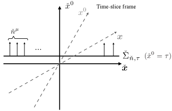
A schematic figure is given in the left panel in Fig. 1. We can generalize the equal-time foliation of whole Minkowski space 𝐌d+1\mathbf{M}^{d+1} to a general foliation by set n={Σn,τ}τ\mathscr{F}_{n}=\Set{\Sigma_{n,\tau}}_{\tau\in\mathbb{R}} of these spacelike hyperplanes.

Refer to caption
Refer to caption


Figure 1: Σn,τ\Sigma_{n,\tau} in xx frame (left) and Σˇnˇ,τ(=Σn,τ)\check{\Sigma}_{\check{n},\tau}(=\Sigma_{n,\tau}) in xˇ\check{x} frame (right)

In general, we may parametrize a component of nn in the reference frame as the following linear combination:

nμ\displaystyle n^{\mu} =μ(𝒏)νν,\displaystyle=\mathscr{L}^{\mu}{}_{\nu}\!\left(\boldsymbol{n}\right)\ell^{\nu}, (81)

where the “standard vector” \ell is defined to be

(μ)μ=0,,d=(1,𝟎)\displaystyle\left(\ell^{\mu}\right)_{\mu=0,\dots,d}=\left(1,\boldsymbol{0}\right) (82)

in any frame999 In the language of differential geometry, the basis-independent vector is written as nˇ:=nˇμμ\check{n}:=\check{n}^{\mu}\partial_{\mu} with μ=xμ\partial_{\mu}={\partial\over\partial x^{\mu}} being the basis vectors in the reference coordinates. Under the change of basis μμ=Λμνν\partial_{\mu}\to\partial_{\mu}^{\prime}=\Lambda_{\mu}{}^{\nu}\partial_{\nu}, where μ:=xμ\partial^{\prime}_{\mu}:={\partial\over\partial x^{\prime\mu}}, nˇ\check{n} should remain the same nˇnˇμμ=nˇμΛμνν=!nˇνν\check{n}\to\check{n}^{\prime\mu}\partial_{\mu}^{\prime}=\check{n}^{\prime\mu}\Lambda_{\mu}{}^{\nu}\partial_{\nu}\stackrel{{\scriptstyle!}}{{=}}\check{n}^{\nu}\partial_{\nu}, that is, nˇμ=Λμnˇνν\check{n}^{\prime\mu}=\Lambda^{\mu}{}_{\nu}\check{n}^{\nu}. and (𝒏)\mathscr{L}\!\left(\boldsymbol{n}\right) is the “standard boost to the foliation.” Concretely, for the vector with n0=1+𝒏2n^{0}=\sqrt{1+\boldsymbol{n}^{2}},

(𝒏)\displaystyle\mathscr{L}\!\left(\boldsymbol{n}\right) =[n0𝒏t𝒏I+(n01)𝒏𝒏t𝒏2],\displaystyle=\begin{bmatrix}n^{0}&\boldsymbol{n}^{\text{t}}\\ \boldsymbol{n}&\text{I}+\left(n^{0}-1\right){\boldsymbol{n}\boldsymbol{n}^{\text{t}}\over\boldsymbol{n}^{2}}\end{bmatrix}, (83)

where t denotes a transpose, I is the identity matrix in dd dimensions, 𝒏\boldsymbol{n} is given in the n×1n\times 1 matrix representation, and (𝒏)=[μ(𝒏)ν]μ,ν=0,,d\mathscr{L}\!\left(\boldsymbol{n}\right)=\begin{bmatrix}\mathscr{L}^{\mu}{}_{\nu}\!\left(\boldsymbol{n}\right)\end{bmatrix}_{\mu,\nu=0,\dots,d}. Note that 1(𝒏)=(𝒏)\mathscr{L}^{-1}\!\left(\boldsymbol{n}\right)=\mathscr{L}\!\left(-\boldsymbol{n}\right). Now an equal-time hyperplane x0=τx^{0}=\tau in the arbitrary reference frame is written as Σ,τ\Sigma_{\ell,\tau} because x+τ=x0+τ=0\ell\cdot x+\tau=-x^{0}+\tau=0 on it.

For any given foliation n\mathscr{F}_{n}, we may Lorentz-transform from the reference frame xx to the “time-slice” frame xˇ\check{x} that gives nˇμ=μ\check{n}^{\mu}=\ell^{\mu}:

xμ\displaystyle x^{\mu} xˇμ=ν(𝒏)μxν,\displaystyle\to\check{x}^{\mu}=\mathscr{L}_{\nu}{}^{\mu}\!\left(\boldsymbol{n}\right)x^{\nu}, (84)
nμ\displaystyle n^{\mu} nˇμ=ν(𝒏)μnν(=μ),\displaystyle\to\check{n}^{\mu}=\mathscr{L}_{\nu}{}^{\mu}\!\left(\boldsymbol{n}\right)n^{\nu}\quad(=\ell^{\mu}), (85)

where we used (1)=μννμ\left(\mathscr{L}^{-1}\right)\!{}^{\mu}{}_{\nu}=\mathscr{L}_{\nu}{}^{\mu} as usual. In the time-slice coordinate system xˇ\check{x}, the same plane is written as

Σˇnˇ,τ:={xˇ=1(𝒏)x,x1,d|nˇxˇ+τ=0}(=Σn,τ).\displaystyle\check{\Sigma}_{\check{n},\tau}:=\Set{\check{x}=\mathscr{L}^{-1}\!\left(\boldsymbol{n}\right)x,\,x\in\mathbb{R}^{1,d}}{\check{n}\cdot\check{x}+\tau=0}\quad(=\Sigma_{n,\tau}). (86)

As said above, since nˇxˇ+τ=xˇ0+τ=0\check{n}\cdot\check{x}+\tau=-\check{x}^{0}+\tau=0 on Σˇnˇ,τ\check{\Sigma}_{\check{n},\tau}, they are equal-time hyperplanes parametrized by τ\tau\in\mathbb{R} in the xˇ\check{x} coordinate system. A schematic figure is given in the right panel in Fig. 1.

Appendix B Wigner representation

In this appendix, we briefly review the Wigner representation in the case of massive one-particle state |𝒑,s\rrangle\left\lvert\boldsymbol{p},s\right\rrangle to spell out our notation; see e.g. Ref. [1] for more details. Here and hereafter, we neglect the label for the particle and anti-particle since it is irrelevant for the current discussion.

The Poincaré transformation on a plane-wave state can be written as

|p,s\rrangle\displaystyle\left\lvert p,s\right\rrangle U^(Λ,a)|p,s\rrangle\displaystyle\to\widehat{U}\!\left(\Lambda,a\right)\left\lvert p,s\right\rrangle (87)

where

U^(Λ,a)\displaystyle\widehat{U}\!\left(\Lambda,a\right) =eia𝒫^U^(Λ)=eia0H^i𝒂𝓟^U^(Λ),\displaystyle=e^{-ia\cdot\widehat{\mathcal{P}}}\widehat{U}\!\left(\Lambda\right)=e^{ia^{0}\widehat{H}-i\boldsymbol{a}\cdot\boldsymbol{\widehat{\mathcal{P}}}}\widehat{U}\!\left(\Lambda\right), (88)

in which 𝒫^=(𝒫^0,𝓟^)\widehat{\mathcal{P}}=\left(\widehat{\mathcal{P}}^{0},\boldsymbol{\widehat{\mathcal{P}}}\right) is the generator of the spacetime translation. Since the translational part is the same as the scalar case, we concentrate on the Lorentz transformation.

Without loss of generality, we can choose ss to be the of the particle in its rest frame:

|p,s\rrangle\displaystyle\left\lvert p,s\right\rrangle =U^(L(p))|𝟎,s\rrangle,\displaystyle=\widehat{U}\bigl{(}{L\!\left(p\right)}\bigr{)}\left\lvert\boldsymbol{0},s\right\rrangle, (89)

consistently with the definition (8) as we will see below. Here, ss is the spin eigenvalue for the rotation in, say, x1x^{1}-x2x^{2} plane in the rest frame and the standard boost L(p)L\!\left(p\right) is defined by

pμ\displaystyle p^{\mu} =:Lμ(p)νmν,\displaystyle=:L^{\mu}{}_{\nu}\!\left(p\right)m\ell^{\nu}, (90)

in which μ\ell^{\mu} is given in Eq. (82). Concretely, the standard boost to pp can be written in terms of the “standard boost to a foliation” (83) as101010 In general, these two are different concepts, L(𝒑)(𝒏)L\!\left(\boldsymbol{p}\right)\neq\mathscr{L}\!\left(\boldsymbol{n}\right), since 𝒑\boldsymbol{p} and 𝒏\boldsymbol{n} are different.

L(p)\displaystyle L\!\left(p\right) =(p/m).\displaystyle=\mathscr{L}\!\left(p/m\right). (91)

Since |p,s\rrangle\left\lvert p,s\right\rrangle has an internal degree of freedom ss, the Lorentz group representation for this state could be nontrivial. To deal with this, we introduce the well-known procedure, Wigner representation. First, under the Lorentz transformation, the plane-wave basis transforms as

U^(Λ)|p,s\rrangle\displaystyle\widehat{U}\!\left(\Lambda\right)\left\lvert p,s\right\rrangle =U^(Λ)U^(L(p))|𝟎,s\rrangle=U^(L(Λp))U^(L1(Λp))U^(Λ)U^(L(p))|𝟎,s\rrangle\displaystyle=\widehat{U}\!\left(\Lambda\right)\widehat{U}\bigl{(}{L\!\left(p\right)}\bigr{)}\left\lvert\boldsymbol{0},s\right\rrangle=\widehat{U}\bigl{(}{L\!\left(\Lambda p\right)}\bigr{)}\widehat{U}\!\left(L^{-1}\!\left(\Lambda p\right)\right)\widehat{U}\!\left(\Lambda\right)\widehat{U}\bigl{(}{L\!\left(p\right)}\bigr{)}\left\lvert\boldsymbol{0},s\right\rrangle
=U^(L(Λp))U^(W(Λ,p))|𝟎,s\rrangle,\displaystyle=\widehat{U}\bigl{(}{L\!\left(\Lambda p\right)}\bigr{)}\widehat{U}\bigl{(}{W\!\left(\Lambda,p\right)}\bigr{)}\left\lvert\boldsymbol{0},s\right\rrangle, (92)

where

W(Λ,p)\displaystyle W\!\left(\Lambda,p\right) :=L1(Λp)ΛL(p).\displaystyle:=L^{-1}\!\left(\Lambda p\right)\Lambda L\!\left(p\right). (93)

Here, W(Λ,p)W\!\left(\Lambda,p\right) is corresponding to the rotation because this transformation does not change the momentum pp. We call this Wigner rotation in SO(d)SO(d).111111 We sloppily write SO(d)SO(d) when it is to be understood as Spin(d)(d). Next, we may always write

U^(W(Λ,p))|𝟎,s\rrangle\displaystyle\widehat{U}\bigl{(}{W\!\left(\Lambda,p\right)}\bigr{)}\left\lvert\boldsymbol{0},s\right\rrangle =s|𝟎,s\rrangleDss(W(Λ,p)),\displaystyle=\sum_{s^{\prime}}\left\lvert\boldsymbol{0},s^{\prime}\right\rrangle D_{s^{\prime}s}\bigl{(}{W\!\left(\Lambda,p\right)}\bigr{)}, (94)

where DD is a finite-dimensional unitary representation of SO(d)SO(d):

sDs′′s(W(Λ,p))Dss(W(Λ,p))=δss′′.\displaystyle\sum_{s}D_{s^{\prime\prime}s}\bigl{(}{W\!\left(\Lambda,p\right)}\bigr{)}D^{*}_{s^{\prime}s}\bigl{(}{W\!\left(\Lambda,p\right)}\bigr{)}=\delta_{s^{\prime}s^{\prime\prime}}. (95)

Putting Eq. (94) into Eq. (92), we obtain Eq. (10).

Appendix C Energy, momentum, and number operator in scalar case

We give the energy, momentum, and number operators for a real scalar field in terms of the Lorentz-invariant wave-packet basis. First, we briefly review the scalar wave packet in QFT, and then we will show newly-found expressions of these operators in terms of the Lorentz-invariant scalar wave packets.

The free field is usually expressed in the plane wave basis:

ϕ^(x)\displaystyle\widehat{\phi}\!\left(x\right) =dd𝒑2p0(α^(p)eipx(2π)d/2+α^(p)eipx(2π)d/2),\displaystyle=\int{\text{d}^{d}\boldsymbol{p}\over 2p^{0}}\left(\widehat{\alpha}\!\left(p\right){e^{ip\cdot x}\over\left(2\pi\right)^{d/2}}+\widehat{\alpha}^{\dagger}\!\left(p\right){e^{-ip\cdot x}\over\left(2\pi\right)^{d/2}}\right), (96)

where α^(p)\widehat{\alpha}\!\left(p\right) and α^(p)\widehat{\alpha}^{\dagger}\!\left(p\right) are the creation and annihilation operators of the plane waves, which satisfy [α^(p),α^(p)]=2p0δd(𝒑𝒑)\left[\widehat{\alpha}\!\left(p\right)\,,\>\widehat{\alpha}^{\dagger}\!\left(p^{\prime}\right)\right]=2p^{0}\,\delta^{d}\!\left(\boldsymbol{p}-\boldsymbol{p}^{\prime}\right), etc.

Now, we define a wave-packet creation operator by [26]

A^(Π)|0:=|Π\rrangle,\displaystyle\widehat{A}^{\dagger}\!\left(\Pi\right)\ket{0}:=\left\lvert\Pi\right\rrangle, (97)

and an annihilation operator A^(Π)\widehat{A}\!\left(\Pi\right) by its Hermitian conjugate. The completeness of the scalar wave packet (22) leads to the following expansion of the creation and annihilation operators of the plane waves:

α^(p)\displaystyle\widehat{\alpha}\!\left(p\right) =d2dΠ\llanglep|Π\rrangleA^(Π),\displaystyle=\int\text{d}^{2d}\Pi\left\llangle p\mathchoice{\;}{\;}{\,}{\,}\middle|\mathchoice{\;}{\;}{\,}{\,}\Pi\right\rrangle\widehat{A}\!\left(\Pi\right), α^(p)\displaystyle\widehat{\alpha}^{\dagger}\!\left(p\right) =d2dΠA^(Π)\llangleΠ|p\rrangle.\displaystyle=\int\text{d}^{2d}\Pi\,\widehat{A}^{\dagger}\!\left(\Pi\right)\left\llangle\Pi\mathchoice{\;}{\;}{\,}{\,}\middle|\mathchoice{\;}{\;}{\,}{\,}p\right\rrangle. (98)

Thus, the free scalar field can be expanded as [26]

ϕ^(x)\displaystyle\widehat{\phi}\!\left(x\right) =d2dΠ[\llanglex|Π\rrangleA^(Π)+A^(Π)\llangleΠ|x\rrangle],\displaystyle=\int\text{d}^{2d}\Pi\left[\left\llangle x\mathchoice{\;}{\;}{\,}{\,}\middle|\mathchoice{\;}{\;}{\,}{\,}\Pi\right\rrangle\widehat{A}\!\left(\Pi\right)+\widehat{A}^{\dagger}\!\left(\Pi\right)\left\llangle\Pi\mathchoice{\;}{\;}{\,}{\,}\middle|\mathchoice{\;}{\;}{\,}{\,}x\right\rrangle\right], (99)

where the wave function is given in Eq. (14).

Now let us rewrite well-known operators in QFT, i.e. the total Hamiltonian, momentum, and number operators, into the language of the scalar wave packet.

First, in momentum space, the convergent part of the number operator is described by

N^:=dd𝒑2p0α^(p)α^(p).\displaystyle\widehat{N}:=\int{\text{d}^{d}\boldsymbol{p}\over 2p^{0}}\widehat{\alpha}^{\dagger}\!\left(p\right)\widehat{\alpha}\!\left(p\right). (100)

Substituting Eq. (98) into the above expression, we obtain

N^\displaystyle\widehat{N} =d2dΠd2dΠA^(Π)\llangleΠ|Π\rrangleA^(Π)\displaystyle=\int\text{d}^{2d}\Pi\,\int\text{d}^{2d}\Pi^{\prime}\,\widehat{A}^{\dagger}\!\left(\Pi\right)\left\llangle\Pi\mathchoice{\;}{\;}{\,}{\,}\middle|\mathchoice{\;}{\;}{\,}{\,}\Pi^{\prime}\right\rrangle\widehat{A}\!\left(\Pi^{\prime}\right)
=d2dΠA^(Π)A^(Π).\displaystyle=\int\text{d}^{2d}\Pi\,\widehat{A}^{\dagger}\!\left(\Pi\right)\widehat{A}\!\left(\Pi\right). (101)

On the second line, we have used

A^(Π)=d2dΠ\llangleΠ|Π\rrangleA^(Π),\displaystyle\widehat{A}\!\left(\Pi\right)=\int\text{d}^{2d}\Pi^{\prime}\left\llangle\Pi\mathchoice{\;}{\;}{\,}{\,}\middle|\mathchoice{\;}{\;}{\,}{\,}\Pi^{\prime}\right\rrangle\widehat{A}\!\left(\Pi^{\prime}\right), A^(Π)=d2dΠA^(Π)\llangleΠ|Π\rrangle,\displaystyle\widehat{A}^{\dagger}\!\left(\Pi\right)=\int\text{d}^{2d}\Pi^{\prime}\widehat{A}^{\dagger}\!\left(\Pi^{\prime}\right)\left\llangle\Pi^{\prime}\mathchoice{\;}{\;}{\,}{\,}\middle|\mathchoice{\;}{\;}{\,}{\,}\Pi\right\rrangle, (102)

which follows from Eq. (22). From Eq. (101), we can read off a Lorentz-covariant number-density operator in the 2d2d-dimensional phase space:

𝒩^=A^(Π)A^(Π).\displaystyle\widehat{\mathcal{N}}=\widehat{A}^{\dagger}\!\left(\Pi\right)\widehat{A}\!\left(\Pi\right). (103)

We now consider the divergent part of the plane-wave number operator, coming from the zero-point oscillation:

N^zero:=dd𝒑2p012[α^(p),α^(p)].\displaystyle\widehat{N}_{\mathrm{zero}}:=\int{\text{d}^{d}\boldsymbol{p}\over 2p^{0}}\frac{1}{2}\left[\widehat{\alpha}\!\left(p\right)\,,\>\widehat{\alpha}^{\dagger}\!\left(p\right)\right]. (104)

Putting Eq. (98) into the above expression, we obtain

N^zero\displaystyle\widehat{N}_{\mathrm{zero}} =d2dΠd2dΠ12\llangleΠ|Π\rrangle\llangleΠ|Π\rrangle1^\displaystyle=\int\text{d}^{2d}\Pi\,\int\text{d}^{2d}\Pi^{\prime}\,\frac{1}{2}\left\llangle\Pi\mathchoice{\;}{\;}{\,}{\,}\middle|\mathchoice{\;}{\;}{\,}{\,}\Pi^{\prime}\right\rrangle\left\llangle\Pi^{\prime}\mathchoice{\;}{\;}{\,}{\,}\middle|\mathchoice{\;}{\;}{\,}{\,}\Pi\right\rrangle\widehat{1}
=12d2dΠ1^.\displaystyle=\frac{1}{2}\int\text{d}^{2d}\Pi\,\widehat{1}. (105)

Therefore, including the divergent part, the number-density operator can be described by

𝒩^+𝒩^zero:=A^(Π)A^(Π)+12\displaystyle\widehat{\mathcal{N}}+\widehat{\mathcal{N}}_{\mathrm{zero}}:=\widehat{A}^{\dagger}\!\left(\Pi\right)\widehat{A}\!\left(\Pi\right)+\frac{1}{2} (106)

From this expression, it can be interpreted that there is one zero-point oscillation per 2d2d-dimensional phase space volume.

Next, we consider the convergent part of the total Hamiltonian and momentum operators. In the momentum space, these operators are given by

P^μ:=dd𝒑2p0pμα^(p)α^(p).\displaystyle\widehat{P}^{\mu}:=\int{\text{d}^{d}\boldsymbol{p}\over 2p^{0}}p^{\mu}\widehat{\alpha}^{\dagger}\!\left(p\right)\widehat{\alpha}\!\left(p\right). (107)

Putting Eq. (98) into the above expression, we get

P^μ\displaystyle\widehat{P}^{\mu} =d2dΠd2dΠA^(Π)A^(Π)\llanglep^μ\rrangleΠ,Π,\displaystyle=\int\text{d}^{2d}\Pi\int\text{d}^{2d}\Pi^{\prime}\,\widehat{A}^{\dagger}\!\left(\Pi\right)\widehat{A}\!\left(\Pi^{\prime}\right)\left\llangle\hat{p}^{\mu}\right\rrangle_{\Pi,\Pi^{\prime}}, (108)

where \llanglep^μ\rrangleΠ,Π\left\llangle\hat{p}^{\mu}\right\rrangle_{\Pi,\Pi^{\prime}} is given in Eq.(21). We see that the total Hamiltonian and momentum operators are not diagonal on the wave packet basis, unlike the plane-wave eigenbasis.

Now, let us discuss the divergent part of this operator, coming from the zero-point energy:

P^zeroμ:=dd𝒑2p0pμ12[α^(p),α^(p)].\displaystyle\widehat{P}^{\mu}_{\mathrm{zero}}:=\int{\text{d}^{d}\boldsymbol{p}\over 2p^{0}}p^{\mu}\frac{1}{2}\left[\widehat{\alpha}\!\left(p\right)\,,\>\widehat{\alpha}^{\dagger}\!\left(p\right)\right]. (109)

Putting Eq. (98) into the above commutator, we obtain

P^zeroμ\displaystyle\widehat{P}^{\mu}_{\mathrm{zero}} =12d2dΠ(Π)d2dΠ\llanglep^μ\rrangleΠ,Π\llangleΠ|Π\rrangle1^\displaystyle=\frac{1}{2}\int\text{d}^{2d}\Pi\,\!\left(\Pi\right)\int\text{d}^{2d}\Pi^{\prime}\,\left\llangle\hat{p}^{\mu}\right\rrangle_{\Pi,\Pi^{\prime}}\left\llangle\Pi^{\prime}\mathchoice{\;}{\;}{\,}{\,}\middle|\mathchoice{\;}{\;}{\,}{\,}\Pi\right\rrangle\widehat{1}
=12d2dΠ\llanglep^μ\rrangleϕ1^,\displaystyle=\frac{1}{2}\int\text{d}^{2d}\Pi\,\left\llangle\hat{p}^{\mu}\right\rrangle_{\phi}\widehat{1},
=dd+1X(2π)ddd𝑷2P0(PN)δ(NX+T)Pμ1^\displaystyle=\int\frac{\text{d}^{d+1}X}{(2\pi)^{d}}{\text{d}^{d}\boldsymbol{P}\over 2P^{0}}\left(-P\cdot N\right)\,\delta\!\left(N\cdot X+T\right)P^{\mu}\,\widehat{1}
=dd+1X(2π)ddd𝑷2P0(PN)2δ(NX+T)Nμ1^.\displaystyle=\int\frac{\text{d}^{d+1}X}{(2\pi)^{d}}{\text{d}^{d}\boldsymbol{P}\over 2P^{0}}\left(P\cdot N\right)^{2}\,\delta\!\left(N\cdot X+T\right)N^{\mu}\,\widehat{1}. (110)

where we have used the completeness relation (22) in the second line, the formula (18) in the third line, and the same argument as in Eq. (73) in the last line. It is noteworthy that the result becomes the same as in the spinor case (71) up to the factor 4-4.

We may define the zero-point energy in a manifestly Lorentz-invariant fashion:

Ezero\displaystyle E_{\mathrm{zero}} :=NμPzeroμ\displaystyle:=-N_{\mu}P_{\mathrm{zero}}^{\mu}
=dd+1X(2π)ddd𝑷2P0(PN)2δ(NX+T),\displaystyle=\int\frac{\text{d}^{d+1}X}{(2\pi)^{d}}{\text{d}^{d}\boldsymbol{P}\over 2P^{0}}\left(P\cdot N\right)^{2}\,\delta\!\left(N\cdot X+T\right), (111)

where PzeroμP_{\mathrm{zero}}^{\mu} is the coefficient of 1^\widehat{1} in the right-hand side of Eq. (110).

Physically, we expect that the zero-point energy should be independent of the choice of the spacelike hyperplane ΣN,T\Sigma_{N,T}. We can show it by exploiting the Lorentz invariance of the expression (111) to choose Nμ=μN^{\mu}=\ell^{\mu} (=(1,𝟎)=\left(1,\boldsymbol{0}\right)), without loss of generality. Then, the zero-point energy reduces to the well-known form:

Ezero=X0=Tdd𝑿dd𝑷(2π)d12P0.\displaystyle E_{\mathrm{zero}}=\int_{X^{0}=T}{\text{d}^{d}\boldsymbol{X}\,\text{d}^{d}\boldsymbol{P}\over\left(2\pi\right)^{d}}\frac{1}{2}P^{0}. (112)

Appendix D Conversion of metric convention

We list the corresponding equations in the almost-minus metric signature (+,,,)\left(+,-,\dots,-\right) to those in the main text. In this paragraph only, we tentatively put the subscript “Main” and “AppD” on those in the main text and Appdendix D, respectively. The metric sign is reverted: ηAppD=diag(1,1,,1)\eta_{\text{AppD}}=\operatorname{diag}\!\left(1,-1,\dots,-1\right), and β=γAppD0\beta=\gamma^{0}_{\text{AppD}}; see footnote 1. The gamma matrices are related by γMainμ=iγAppDμ\gamma^{\mu}_{\text{Main}}=-i\gamma^{\mu}_{\text{AppD}}. The Clifford algebra remains the same: {γAppDμ,γAppDν}=2ηAppDμνI\{\gamma_{\text{AppD}}^{\mu},\gamma_{\text{AppD}}^{\nu}\}=2\eta^{\mu\nu}_{\text{AppD}}I.

Section 1

Eq. (1) becomes

\llanglep,s|X,P,S;σ\rrangle\displaystyle\left\llangle p,s\mathchoice{\;}{\;}{\,}{\,}\middle|\mathchoice{\;}{\;}{\,}{\,}X,P,S;\sigma\right\rrangle eip(X+iσP)u¯(p,s)u(P,S)\displaystyle\propto e^{ip\cdot\left(X+i\sigma P\right)}\overline{u}\!\left(p,s\right)u\!\left(P,S\right)
=eip(X+iσP)v¯(P,S)v(p,s).\displaystyle\quad=-e^{ip\cdot\left(X+i\sigma P\right)}\overline{v}\!\left(P,S\right)v\!\left(p,s\right). (113)

Section 2

Eq. (2) becomes

ψ^(x)\displaystyle\widehat{\psi}\!\left(x\right) =sdd𝒑2p0(u(p,s)eipx(2π)d/2α^(p,s)+v(p,s)eipx(2π)d/2β^(p,s)).\displaystyle=\sum_{s}\int{\text{d}^{d}\boldsymbol{p}\over 2p^{0}}\left(u(p,s){e^{-ip\cdot x}\over\left(2\pi\right)^{d/2}}\widehat{\alpha}\!\left(p,s\right)+v(p,s){e^{ip\cdot x}\over\left(2\pi\right)^{d/2}}\widehat{\beta}^{\dagger}\!\left(p,s\right)\right). (114)

Eq. (3) becomes

(m)u(p,s)=0,\displaystyle(\not{p}-m)u(p,s)=0,
(+m)v(p,s)=0.\displaystyle(\not{p}+m)v(p,s)=0. (115)

Eq. (4) becomes

su(p,s)u¯(p,s)\displaystyle\sum_{s}u(p,s)\overline{u}(p,s) =+m,\displaystyle=\not{p}+m,
sv(p,s)v¯(p,s)\displaystyle\sum_{s}v(p,s)\overline{v}(p,s) =m.\displaystyle=\not{p}-m. (116)

Eq. (5) is unchanged; hereafter, we do not mention unchanged equations. Eq. (11) becomes

\llanglep|Π\rrangle\displaystyle\left\llangle p\mathchoice{\;}{\;}{\,}{\,}\middle|\mathchoice{\;}{\;}{\,}{\,}\Pi\right\rrangle :=Nϕeip(X+iσP).\displaystyle:=N_{\phi}e^{ip\cdot\left(X+i\sigma P\right)}. (117)

The “Lorentzian norm” becomes

V:=V2,\displaystyle\left\|V\right\|:=\sqrt{V^{2}}, (118)

and with the same definition ξμ:=m[σPμ+i(xX)μ]\xi^{\mu}:=m\left[\sigma P^{\mu}+i\left(x-X\right)^{\mu}\right] and Ξμ:=m[σ(P+P)μ+i(XX)μ]\Xi^{\mu}:=m\left[\sigma\left(P+P^{\prime}\right)^{\mu}+i\left(X-X^{\prime}\right)^{\mu}\right], Eqs. (16) and (17) becomes

ξ\displaystyle\left\|\xi\right\| =mσ2m2(xX)2+2iσP(xX),\displaystyle=m\sqrt{\sigma^{2}m^{2}-\left(x-X\right)^{2}+2i\sigma P\cdot\left(x-X\right)}, (119)
Ξ\displaystyle\left\|\Xi\right\| =m((XX)iσ(P+P))2.\displaystyle=m\sqrt{-\bigl{(}\left(X-X^{\prime}\right)-i\sigma\left(P+P^{\prime}\right)\bigr{)}^{2}}. (120)

Eq. (19) becomes

\llanglep^μp^ν\rrangleϕ\displaystyle\left\llangle\hat{p}^{\mu}\hat{p}^{\nu}\right\rrangle_{\phi} =Kd+32(2σm2)Kd12(2σm2)PμPνϕ2σημν.\displaystyle={K_{d+3\over 2}\!\left(2\sigma m^{2}\right)\over K_{d-1\over 2}\!\left(2\sigma m^{2}\right)}P^{\mu}P^{\nu}-{\mathcal{M}_{\phi}\over 2\sigma}\eta^{\mu\nu}. (121)

The spacelike hyperplane becomes ΣN,T={X|NXT=0}\Sigma_{N,T}=\Set{X}{N\cdot X-T=0}. Eq. (23) becomes

d2dΠϕ\displaystyle\int\text{d}^{2d}\Pi_{\phi} :=1ϕddΣXμ(2π)d(2Pμ)dd𝑷2P0.\displaystyle:={1\over\mathcal{M}_{\phi}}\int{\text{d}^{d}\Sigma^{\mu}_{X}\over\left(2\pi\right)^{d}}\left(2P_{\mu}\right){\text{d}^{d}\boldsymbol{P}\over 2P^{0}}. (122)

Eq. (24) becomes

ddΣXμ\displaystyle\text{d}^{d}\Sigma^{\mu}_{X} :=dd+1Xδ(NXT)Nμ.\displaystyle:=\text{d}^{d+1}X\,\delta\!\left(N\cdot X-T\right)N^{\mu}. (123)

Eq. (34) reads

\llanglep,s,N|Π,S,N\rrangle:=Nψeip(X+iσP)MsS(p,P,N)δNN.\displaystyle\left\llangle p,s,N\mathchoice{\;}{\;}{\,}{\,}\middle|\mathchoice{\;}{\;}{\,}{\,}\Pi,S,N^{\prime}\right\rrangle:=N_{\psi}e^{ip\cdot\left(X+i\sigma P\right)}M_{sS}\!\left(p,P,N\right)\delta_{NN^{\prime}}. (124)

The charge conjugation matrix becomes C=iγ2C=-i\gamma^{2} with C=Ct=C=CC^{*}=C^{\text{t}}=C^{\dagger}=C. Eq. (40) becomes

\llangleΠ,S|Π,S\rrangle\displaystyle\left\llangle\Pi,S\mathchoice{\;}{\;}{\,}{\,}\middle|\mathchoice{\;}{\;}{\,}{\,}\Pi,S\right\rrangle =Nψ2(2m)2u¯(P,S)(dd𝒑2p0\llangleΠ|p\rrangle\llanglep|Π\rrangleNϕ2(+m))u(P,S)\displaystyle={N_{\psi}^{2}\over\left(2m\right)^{2}}\overline{u}\!\left(P,S\right)\left(\int{\text{d}^{d}\boldsymbol{p}\over 2p^{0}}{\left\llangle\Pi\mathchoice{\;}{\;}{\,}{\,}\middle|\mathchoice{\;}{\;}{\,}{\,}p\right\rrangle\left\llangle p\mathchoice{\;}{\;}{\,}{\,}\middle|\mathchoice{\;}{\;}{\,}{\,}\Pi\right\rrangle\over N_{\phi}^{2}}\left(\not{p}+m\right)\right)u\!\left(P,S\right)
=Nψ2(2m)2u¯(P,S)\llanglep^+m\rrangleϕNϕ2u(P,S)\displaystyle={N_{\psi}^{2}\over\left(2m\right)^{2}}\overline{u}\!\left(P,S\right){\left\llangle\not{\hat{p}}+m\right\rrangle_{\phi}\over N_{\phi}^{2}}u\!\left(P,S\right)
(=Nψ2(2m)2v¯(P,S)\llanglep^m\rrangleϕNϕ2v(P,S)).\displaystyle\left(={N_{\psi}^{2}\over\left(2m\right)^{2}}\overline{v}\!\left(P,S\right){\left\llangle\not{\hat{p}}-m\right\rrangle_{\phi}\over N_{\phi}^{2}}v\!\left(P,S\right)\right). (125)

Eq. (41) becomes

\llanglep^±m\rrangleϕ=ϕ±m.\displaystyle\left\llangle\not{\hat{p}}\pm m\right\rrangle_{\phi}=\mathcal{M}_{\phi}\not{P}\pm m. (126)

Eq. (42) becomes

\llangleΠ,S|Π,S\rrangle\displaystyle\left\llangle\Pi,S\mathchoice{\;}{\;}{\,}{\,}\middle|\mathchoice{\;}{\;}{\,}{\,}\Pi^{\prime},S^{\prime}\right\rrangle =Nψ2(2m)2u¯(P,S)\llanglep^+m\rrangleΠ,ΠNϕ2u(P,S)δnn\displaystyle={N_{\psi}^{2}\over\left(2m\right)^{2}}\overline{u}\!\left(P,S\right){\left\llangle\not{\hat{p}}+m\right\rrangle_{\Pi,\Pi^{\prime}}\over N_{\phi}^{2}}u\!\left(P^{\prime},S^{\prime}\right)\delta_{nn^{\prime}}
(=Nψ2(2m)2v¯(P,S)\llanglep^m\rrangleΠ,ΠNϕ2v(P,S)δncnc).\displaystyle\left(={N_{\psi}^{2}\over\left(2m\right)^{2}}\overline{v}\!\left(P,S\right){\left\llangle\not{\hat{p}}-m\right\rrangle_{\Pi,\Pi^{\prime}}\over N_{\phi}^{2}}v\!\left(P^{\prime},S^{\prime}\right)\delta_{n^{\text{c}}n^{\prime\text{c}}}\right). (127)

Eq. (44) becomes

\llanglep^μ\rrangleψ\displaystyle\left\llangle\hat{p}^{\mu}\right\rrangle_{\psi} =Nψ4m2u¯(P,S)\llanglep^μ(p^+m)\rrangleϕNϕ2u(P,S)(=Nψ4m2v¯(P,S)\llanglep^μ(p^m)\rrangleϕNϕ2v(P,S)).\displaystyle={N_{\psi}\over 4m^{2}}\overline{u}(P,S){\left\llangle\hat{p}^{\mu}\left(\not{\hat{p}}+m\right)\right\rrangle_{\phi}\over N_{\phi}^{2}}u(P,S)\ \left(={N_{\psi}\over 4m^{2}}\overline{v}(P,S){\left\llangle\hat{p}^{\mu}\left(\not{\hat{p}}-m\right)\right\rrangle_{\phi}\over N_{\phi}^{2}}v(P,S)\right). (128)

Eq. (45) becomes

\llanglep^μ(p^±m)\rrangleϕ\displaystyle\left\llangle\hat{p}^{\mu}\left(\not{\hat{p}}\pm m\right)\right\rrangle_{\phi} =(Kd+32(2σm2)Kd12(2σm2)Pμ+ϕ2σγμ)±ϕmPμ.\displaystyle=\left({K_{d+3\over 2}\!\left(2\sigma m^{2}\right)\over K_{d-1\over 2}\!\left(2\sigma m^{2}\right)}P^{\mu}\not{P}+{\mathcal{M}_{\phi}\over 2\sigma}\gamma^{\mu}\right)\pm\mathcal{M}_{\phi}mP^{\mu}. (129)

Eq. (46) becomes

14m2u¯(P,S)\llanglep^μ(p^+m)\rrangleϕu(P,S)\displaystyle{1\over 4m^{2}}\overline{u}(P,S)\left\llangle\hat{p}^{\mu}\left(\not{\hat{p}}+m\right)\right\rrangle_{\phi}u(P,S) =12(ϕ+ϕ2σm2+Kd+32(2σm2)Kd12(2σm2))Pμ,\displaystyle={1\over 2}\left(\mathcal{M}_{\phi}+{\mathcal{M}_{\phi}\over 2\sigma m^{2}}+{K_{d+3\over 2}\!\left(2\sigma m^{2}\right)\over K_{d-1\over 2}\!\left(2\sigma m^{2}\right)}\right)P^{\mu},
14m2v¯(P,S)\llanglep^μ(p^m)\rrangleϕv(P,S)\displaystyle{1\over 4m^{2}}\overline{v}(P,S)\left\llangle\hat{p}^{\mu}\left(\not{\hat{p}}-m\right)\right\rrangle_{\phi}v(P,S) =12(ϕ+ϕ2σm2+Kd+32(2σm2)Kd12(2σm2))Pμ.\displaystyle={1\over 2}\left(\mathcal{M}_{\phi}+{\mathcal{M}_{\phi}\over 2\sigma m^{2}}+{K_{d+3\over 2}\!\left(2\sigma m^{2}\right)\over K_{d-1\over 2}\!\left(2\sigma m^{2}\right)}\right)P^{\mu}. (130)

Eq. (2.4) becomes

d2dΠψ\displaystyle\int\text{d}^{2d}\Pi_{\psi} :=1ψΣN,TddΣXμ(2π)d(2Pμ)dd𝑷2P0\displaystyle:={1\over\mathcal{M}_{\psi}}\int_{\Sigma_{N,T}}{\text{d}^{d}\Sigma^{\mu}_{X}\over\left(2\pi\right)^{d}}\left(2P_{\mu}\right){\text{d}^{d}\boldsymbol{P}\over 2P^{0}}
=ϕψd2dΠϕ,\displaystyle={\mathcal{M}_{\phi}\over\mathcal{M}_{\psi}}\int\text{d}^{2d}\Pi_{\phi}, (131)

Eq. (51) becomes

Nψ2ψΣN,Tdd+1X(2π)dδ(NXT)(2PN)dd𝑷2P0\llanglep|Π\rrangle\llangleΠ|q\rrangleNϕ2\displaystyle\quad{N_{\psi}^{2}\over\mathcal{M}_{\psi}}\int_{\Sigma_{N,T}}{\text{d}^{d+1}X\over\left(2\pi\right)^{d}}\delta\!\left(N\cdot X-T\right)\left(2P\cdot N\right){\text{d}^{d}\boldsymbol{P}\over 2P^{0}}{\left\llangle p\mathchoice{\;}{\;}{\,}{\,}\middle|\mathchoice{\;}{\;}{\,}{\,}\Pi\right\rrangle\left\llangle\Pi\mathchoice{\;}{\;}{\,}{\,}\middle|\mathchoice{\;}{\;}{\,}{\,}q\right\rrangle\over N_{\phi}^{2}}
×14m2Su¯(p,s)u(P,S)u¯(P,S)u(q,s)\displaystyle\qquad\times\displaystyle{1\over 4m^{2}}\sum_{S}\overline{u}\!\left(p,s\right)u\!\left(P,S\right)\overline{u}\!\left(P,S\right)u\!\left(q,s^{\prime}\right)
=2p0δd(𝒑𝒒)δss.\displaystyle=2p^{0}\delta^{d}(\boldsymbol{p}-\boldsymbol{q})\delta_{ss^{\prime}}. (132)

Eq. (52) becomes

(l.h.s.)\displaystyle(\text{l.h.s.}) =Nψ2ψ2δd(𝒑𝒒)dd𝑷2P02P0e2σPpNϕ2u¯(p,s)(+m)u(p,s)4m2\displaystyle={N_{\psi}^{2}\over\mathcal{M}_{\psi}^{2}}\delta^{d}(\boldsymbol{p}-\boldsymbol{q})\int{\text{d}^{d}\boldsymbol{P}\over 2P^{0}}2P^{0}{e^{2\sigma P\cdot p}\over N_{\phi}^{2}}{\overline{u}\!\left(p,s\right)\left(\not{P}+m\right)u\!\left(p,s^{\prime}\right)\over 4m^{2}}
=Nψ2ψ2δd(𝒑𝒒)u¯(p,s)\llangle2p^0(p^+m)\rrangleϕNϕ2u(q,s)\displaystyle={N_{\psi}^{2}\over\mathcal{M}_{\psi}^{2}}\delta^{d}(\boldsymbol{p}-\boldsymbol{q})\overline{u}\!\left(p,s\right){\left\llangle 2\hat{p}^{0}\left(\not{\hat{p}}+m\right)\right\rrangle_{\phi}\over N_{\phi}^{2}}u\!\left(q,s^{\prime}\right)
=2p0δd(𝒑𝒒).\displaystyle=2p^{0}\delta^{d}(\boldsymbol{p}-\boldsymbol{q}). (133)

Section 3

Eq. (64) becomes

U(x,Π,S)\displaystyle U(x,\Pi,S) =sdd𝒑2p0u(p,s)eipx(2π)d2\llanglep,s|Π,S\rrangle\displaystyle=\sum_{s}\int{\text{d}^{d}\boldsymbol{p}\over 2p^{0}}u\!\left(p,s\right){e^{-ip\cdot x}\over\left(2\pi\right)^{d\over 2}}\left\llangle p,s\mathchoice{\;}{\;}{\,}{\,}\middle|\mathchoice{\;}{\;}{\,}{\,}\Pi,S\right\rrangle
=12mNψNϕ\llanglex|(p^+m)|Π\rrangleu(P,S)\displaystyle={1\over 2m}{N_{\psi}\over N_{\phi}}\left\llangle x\right\rvert\left(\not{\hat{p}}+m\right)\left\lvert\Pi\right\rrangle u\!\left(P,S\right)
=12Nψmd12π(ξ̸Kd+12(ξ)ξd+12+Kd12(ξ)ξd12)u(P,S),\displaystyle={1\over 2}{N_{\psi}m^{d-1}\over\sqrt{2\pi}}\left(\not{\xi}{K_{d+1\over 2}\!\left(\left\|\xi\right\|\right)\over\left\|\xi\right\|^{d+1\over 2}}+{K_{d-1\over 2}\!\left(\left\|\xi\right\|\right)\over\left\|\xi\right\|^{d-1\over 2}}\right)u(P,S), (134)
V(x,Π,S)\displaystyle V(x,\Pi,S) =sdd𝒑2p0v(p,s)eipx(2π)d2\llangleΠ,S|p,s\rrangle\displaystyle=\sum_{s}\int{\text{d}^{d}\boldsymbol{p}\over 2p^{0}}v\!\left(p,s\right){e^{ip\cdot x}\over\left(2\pi\right)^{d\over 2}}\left\llangle\Pi,S\mathchoice{\;}{\;}{\,}{\,}\middle|\mathchoice{\;}{\;}{\,}{\,}p,s\right\rrangle
=CU(x,Π,S).\displaystyle=CU^{*}(x,\Pi,S). (135)

Eq. (65) becomes

dd+1X(2π)dδ(NXT)U¯(x,Π,S)U(x,Π,S)=2mδSS,\displaystyle\int\frac{d^{d+1}X}{(2\pi)^{d}}\delta(N\cdot X-T)\overline{U}(x,\Pi,S)~{}U(x,\Pi,S^{\prime})=2m\delta_{SS^{\prime}},
dd+1X(2π)dδ(NXT)V¯(x,Π,S)V(x,Π,S)=2mδSS.\displaystyle\int\frac{d^{d+1}X}{(2\pi)^{d}}\delta(N\cdot X-T)\overline{V}(x,\Pi,S)~{}V(x,\Pi,S^{\prime})=-2m\delta_{SS^{\prime}}. (136)

Eq. (66) becomes

Sdd+1X(2π)dδ(NXT)U(x,Π,S)U¯(x,Π,S)=ψ+m,\displaystyle\sum_{S}\int\frac{d^{d+1}X}{(2\pi)^{d}}\delta(N\cdot X-T)U(x,\Pi,S)~{}\overline{U}(x,\Pi,S)=\not{P}\mathcal{M}_{\psi}+m,
Sdd+1X(2π)dδ(NXT)V(x,Π,S)V¯(x,Π,S)=ψm.\displaystyle\sum_{S}\int\frac{d^{d+1}X}{(2\pi)^{d}}\delta(N\cdot X-T)V(x,\Pi,S)~{}\overline{V}(x,\Pi,S)=\not{P}\mathcal{M}_{\psi}-m. (137)

Section 4

Eq. (71) becomes

P^zeroμ\displaystyle\widehat{P}^{\mu}_{\mathrm{zero}} =S,Sd2dΠψd2dΠψ\llangle2p^μ\rrangle(Π,S),(Π,S)\llangleΠ,S|Π,S\rrangle1^\displaystyle=\sum_{S,S^{\prime}}\int\text{d}^{2d}\Pi_{\psi}\int\text{d}^{2d}\Pi^{\prime}_{\psi}\,\left\llangle-2\hat{p}^{\mu}\right\rrangle_{(\Pi,S),(\Pi^{\prime},S^{\prime})}\left\llangle\Pi^{\prime},S^{\prime}\mathchoice{\;}{\;}{\,}{\,}\middle|\mathchoice{\;}{\;}{\,}{\,}\Pi,S\right\rrangle\widehat{1}
=Sd2dΠψ\llangle2p^μ\rrangleψ1^\displaystyle=\sum_{S}\int\text{d}^{2d}\Pi_{\psi}\,\left\llangle-2\hat{p}^{\mu}\right\rrangle_{\psi}\widehat{1}
=Sdd+1X(2π)ddd𝑷2P0(2PN)δ(NXT)Pμ1^.\displaystyle=\sum_{S}\int\frac{\text{d}^{d+1}X}{(2\pi)^{d}}{\text{d}^{d}\boldsymbol{P}\over 2P^{0}}\left(-2P\cdot N\right)\,\delta\!\left(N\cdot X-T\right)P^{\mu}\,\widehat{1}. (138)

Eq. (72) becomes

Pμ=(PN)Nμi(PNi)Niμ.\displaystyle P^{\mu}=\left(P\cdot N\right)N^{\mu}-\sum_{i}\left(P\cdot N_{\perp i}\right)N_{\perp i}^{\mu}. (139)

Eq. (74) becomes

Ezero\displaystyle E_{\mathrm{zero}} :=NμPzeroμ\displaystyle:=N_{\mu}P^{\mu}_{\mathrm{zero}}
=Sdd+1X(2π)ddd𝑷2P0(2)(PN)2δ(NXT).\displaystyle=\sum_{S}\int\frac{\text{d}^{d+1}X}{(2\pi)^{d}}{\text{d}^{d}\boldsymbol{P}\over 2P^{0}}\left(-2\right)\left(P\cdot N\right)^{2}\,\delta\!\left(N\cdot X-T\right). (140)

References

  • [1] S. Weinberg, The Quantum theory of fields. Vol. 1: Foundations. Cambridge University Press, 2005.
  • [2] K. Ishikawa, O. Jinnouchi, K. Nishiwaki, and K.-y. Oda, Wave-packet effects: a solution for isospin anomalies in vector-meson decay, Eur. Phys. J. C 83 (2023), no. 10 978, [arXiv:2308.09933].
  • [3] K. Ishikawa, O. Jinnouchi, A. Kubota, T. Sloan, T. H. Tatsuishi, and R. Ushioda, On experimental confirmation of the corrections to Fermi’s golden rule, PTEP 2019 (2019), no. 3 033B02, [arXiv:1901.03019].
  • [4] R. Ushioda, O. Jinnouchi, K. Ishikawa, and T. Sloan, Search for the correction term to the Fermi’s golden rule in positron annihilation, PTEP 2020 (2020), no. 4 043C01, [arXiv:1907.01264].
  • [5] S. Demidov, S. Gninenko, and D. Gorbunov, Light hidden photon production in high energy collisions, JHEP 07 (2019) 162, [arXiv:1812.02719].
  • [6] S. P. Jordan, K. S. M. Lee, and J. Preskill, Quantum Computation of Scattering in Scalar Quantum Field Theories, Quant. Inf. Comput. 14 (2014) 1014–1080, [arXiv:1112.4833].
  • [7] S. P. Jordan, K. S. M. Lee, and J. Preskill, Quantum Algorithms for Quantum Field Theories, Science 336 (2012) 1130–1133, [arXiv:1111.3633].
  • [8] Z. Davoudi, C.-C. Hsieh, and S. V. Kadam, Scattering wave packets of hadrons in gauge theories: Preparation on a quantum computer, arXiv:2402.00840.
  • [9] C. Giunti and C. W. Kim, Coherence of neutrino oscillations in the wave packet approach, Phys. Rev. D 58 (1998) 017301, [hep-ph/9711363].
  • [10] C. Y. Cardall, Coherence of neutrino flavor mixing in quantum field theory, Phys. Rev. D 61 (2000) 073006, [hep-ph/9909332].
  • [11] E. K. Akhmedov, J. Kopp, and M. Lindner, Oscillations of Mossbauer neutrinos, JHEP 05 (2008) 005, [arXiv:0802.2513].
  • [12] J. Kopp, Mossbauer neutrinos in quantum mechanics and quantum field theory, JHEP 06 (2009) 049, [arXiv:0904.4346].
  • [13] E. K. Akhmedov and A. Y. Smirnov, Paradoxes of neutrino oscillations, Phys. Atom. Nucl. 72 (2009) 1363–1381, [arXiv:0905.1903].
  • [14] E. K. Akhmedov and A. Y. Smirnov, Neutrino oscillations: Entanglement, energy-momentum conservation and QFT, Found. Phys. 41 (2011) 1279–1306, [arXiv:1008.2077].
  • [15] E. K. Akhmedov and J. Kopp, Neutrino Oscillations: Quantum Mechanics vs. Quantum Field Theory, JHEP 04 (2010) 008, [arXiv:1001.4815]. [Erratum: JHEP 10, 52 (2013)].
  • [16] J. Wu, J. A. Hutasoit, D. Boyanovsky, and R. Holman, Neutrino Oscillations, Entanglement and Coherence: A Quantum Field theory Study in Real Time, Int. J. Mod. Phys. A 26 (2011) 5261–5297, [arXiv:1002.2649].
  • [17] E. Akhmedov, D. Hernandez, and A. Smirnov, Neutrino production coherence and oscillation experiments, JHEP 04 (2012) 052, [arXiv:1201.4128].
  • [18] M. Blasone, S. De Siena, and C. Matrella, Wave packet approach to quantum correlations in neutrino oscillations, Eur. Phys. J. C 81 (2021), no. 7 660, [arXiv:2104.03166].
  • [19] E. Akhmedov and A. Y. Smirnov, Damping of neutrino oscillations, decoherence and the lengths of neutrino wave packets, JHEP 11 (2022) 082, [arXiv:2208.03736].
  • [20] H. Mitani and K.-y. Oda, Decoherence in neutrino oscillation between 3D Gaussian wave packets, Phys. Lett. B 846 (2023) 138218, [arXiv:2307.12230].
  • [21] K. Ishikawa, K. Nishiwaki, and K.-y. Oda, New effect in wave-packet scattering of quantum fields, Phys. Rev. D 108 (2023), no. 9 096013, [arXiv:2102.12032].
  • [22] P. A. M. Dirac, The quantum theory of the electron, Proc. Roy. Soc. Lond. A 117 (1928) 610–624.
  • [23] C. Becchi, A. Rouet, and R. Stora, The Abelian Higgs-Kibble Model. Unitarity of the S Operator, Phys. Lett. B 52 (1974) 344–346.
  • [24] C. Becchi, A. Rouet, and R. Stora, Renormalization of Gauge Theories, Annals Phys. 98 (1976) 287–321.
  • [25] I. V. Tyutin, Gauge Invariance in Field Theory and Statistical Physics in Operator Formalism, arXiv:0812.0580. Lebedev Institute preprint No. 39 (1975).
  • [26] K.-y. Oda and J. Wada, A complete set of Lorentz-invariant wave packets and modified uncertainty relation, Eur. Phys. J. C 81 (2021), no. 8 751, [arXiv:2104.01798].
  • [27] K. Ishikawa and K.-y. Oda, Particle decay in Gaussian wave-packet formalism revisited, PTEP 2018 (2018), no. 12 123B01, [arXiv:1809.04285].
  • [28] D. V. Naumov and V. A. Naumov, Relativistic wave packets in a field theoretical approach to neutrino oscillations, Russ. Phys. J. 53 (2010) 549–574.
  • [29] D. V. Naumov and V. A. Naumov, A Diagrammatic treatment of neutrino oscillations, J. Phys. G37 (2010) 105014, [arXiv:1008.0306].
  • [30] D. V. Naumov, On the Theory of Wave Packets, Phys. Part. Nucl. Lett. 10 (2013) 642–650, [arXiv:1309.1717].
  • [31] D. Naumov and V. Naumov, Quantum Field Theory of Neutrino Oscillations, Phys. Part. Nucl. 51 (2020), no. 1 1–106.
  • [32] V. A. Naumov and D. S. Shkirmanov, Virtual neutrino propagation at short baselines, Eur. Phys. J. C 82 (2022), no. 8 736, [arXiv:2208.02621].
  • [33] G. Kaiser, Phase Space Approach to Relativistic Quantum Mechanics. 1. Coherent State Representation for Massive Scalar Particles, J. Math. Phys. 18 (1977) 952–959.
  • [34] G. R. Kaiser, Phase Space Approach to Relativistic Quantum Mechanics. 2. Geometrical Aspects, J. Math. Phys. 19 (1978) 502–507.
  • [35] K. Ishikawa, K. Nishiwaki, and K.-y. Oda, Scalar scattering amplitude in the Gaussian wave-packet formalism, PTEP 2020 (2020), no. 10 103B04, [arXiv:2006.14159].
  • [36] A. Edery, Wave packets in QFT: Leading order width corrections to decay rates and clock behavior under Lorentz boosts, Phys. Rev. D 104 (2021), no. 12 125015, [arXiv:2106.13768].
  • [37] I. P. Ivanov, Promises and challenges of high-energy vortex states collisions, Prog. Part. Nucl. Phys. 127 (2022) 103987, [arXiv:2205.00412].