Loosely trapped surface and dynamically transversely trapping surface in Einstein-Maxwell system
Abstract
We study the properties of the loosely trapped surface (LTS) and the dynamically transversely trapping surface (DTTS) in Einstein-Maxwell systems. These concepts of surfaces were proposed by the four of the present authors in order to characterize strong gravity regions. We prove the Penrose-like inequalities for the area of LTSs/DTTSs. Interestingly, although the naively expected upper bound for the area is that of the photon sphere of a Reissner-Nordström black hole with the same mass and charge, the obtained inequalities include corrections represented by the energy density or pressure/tension of electromagnetic fields. Due to this correction, the Penrose-like inequality for the area of LTSs is tighter than the naively expected one. We also evaluate the correction term numerically in the Majumdar-Papapetrou two-black-hole spacetimes.
E0, E31, A13
1 Introduction
Since a black hole creates a strong gravitational field, there exists unstable circular orbits for photons. For a spherically symmetric system, the collection of them makes a surface called a photon sphere. In the Schwarzschild spacetime, for example, the photon sphere exists at the surface , where is the Arnowitt-Deser-Misner (ADM) mass. Furthermore, a generalized concept of a photon sphere, which is called a photon surface, has been proposed Claudel:2000 . However, the definition of the photon surface requires a highly symmetric spacetime (e.g., Yoshino:2016 ). Moreover, the existence of photon surfaces does not necessarily mean that the gravitational field is strong there Claudel:2000 .
A photon sphere is directly related to observational phenomena. The quasinormal modes of black holes are basically determined by the properties of photon spheres cardoso2009 . The black hole shadow, whose direct picture has been taken by the recent radio observations of the Event Horizon Telescope Collaboration akiyama , is also determined by a photon sphere Virbhadra:1999 .
Motivated by the recent observations, the four of the present authors proposed concepts that characterizes strong gravity regions; a loosely trapped surface (LTS) shiromizu2017 , a transversely trapping surface (TTS) Yoshino:2017 , and a dynamically transversely trapping surface (DTTS) Yoshino:2020-1 ; Yoshino:2020-2 (see also Ref. galtsov for an extension of a TTS). For certain cases, we have proved inequalities analogous to the Penrose inequality penrose1973 , that is, their areas are equal to or less than , where is the ADM mass (see also Ref. hod for an earlier work for a photon sphere). The upper bound is realized for a photon sphere in the Schwarzschild black hole, where comes from the areal radius of unstable circular photon orbits. For an LTS, the application is restricted to a spacelike hypersurfaces with a positive Ricci scalar. This restriction is natural because it is guaranteed by the positivity of the energy density for maximally sliced initial data. For a DTTS, on the other hand, one requires the non-positivity of the radial pressure on a DTTS in addition to the positivity of the Ricci scalar. This requirement of the non-positive pressure does not significantly restrict the situation because the vacuum cases do work. However, it remains a little mystery why the non-positivity of the radial pressure is required.
Therefore, in this paper, we shall discuss non-vacuum cases. As a first typical example, we will focus on Einstein-Maxwell systems. We adopt Jang’s work jang1979 to show the inequality, that is, we will employ the method of the inverse mean curvature flow geroch ; wald1977 111The resulted inequality for the minimal surface in Ref. jang1979 has a lower bound. However, it is known that the lower bound is violated for multi-black-hole systems weinstein2004 . The proof for multi-black-hole systems in the Einstein-Maxwell theory is given in Refs. khuri2013 ; khuri2017 .. The upper bound is expected to be given by the area of the outermost photon sphere, i.e., the locus of the unstable circular orbits of photons in a spherically symmetric charged black hole spacetime, namely, a Reissner-Nordström spacetime with the same mass and charge. As a consequence, however, we see that the obtained inequalities depend on (the part of) the energy density and the pressure/tension of the electromagnetic fields which give corrections to the naively expected upper bound. This is impressive because the Penrose inequality for apparent horizons does not depend on such quantities.
The rest of this paper is organized as follows. In Sect. 2, we will briefly describe the Maxwell theory in a curved spacetime. Some of the notations will be explained together. In Sect. 3, we will present the definition of the LTS and prove the Penrose-like inequality in the Einstein-Maxwell system. Then, in Sect. 4, we will present the definition of the DTTS and prove the Penrose-like inequality in the Einstein-Maxwell system. In Sect. 5, we will revisit the problem of DTTSs in Majumdar-Papapetrou two-black-hole spacetimes, which was studied in our previous paper Yoshino:2020-2 , from the viewpoint of the current study. We will examine the properties of the correction term of the Penrose-like inequality through numerical calculations. The last section will give a summary and discussions. In Appendix, we will shortly discuss the case of a TTS defined for static/stationary spacetimes. Note that we use following units in which the speed of light , the Newtonian constant of gravitation and the Coulomb constant , where is the permittivity of vacuum.
2 Einstein-Maxwell theory and setup
In this paper, we consider an asymptotically flat spacelike hypersurface in a four-dimensional spacetime with a metric . We suppose to be the future-directed unit normal to and the induced metric of is given by . In , we consider a two-dimensional closed surface, an LTS (denoted by ) or a DTTS (denoted by ), with the induced metric . The outward unit normal to that surface is (and therefore, ).
We assume the presence of electromagnetic fields on . The electromagnetic fields are specified by the anti-symmetric tensor, , and its Hodge dual, , where is the Levi-Civita symbol in a four-dimensional spacetime. The tensors and follow Maxwell’s equations,
| (1) |
where is the four-current vector. The electric and magnetic fields, and , are defined by
| (2) |
respectively. Obviously, these fields are tangent to because holds. The electric charge density and the electric current are defined by
| (3) |
In our paper, we require the charge density to vanish (outside an LTS or a DTTS), i.e. , but do not necessarily require the electric current to be zero.
The electric and magnetic fields satisfy Gauss’ laws, and , where is the covariant derivative with respect to . The total electric and magnetic charges are
| (4) |
where is a sphere at spacelike infinity and is the outward unit normal to . It would be important to point out that can have a nonzero value even if the electric charge density is zero throughout the spacetime, as one can understand by imagining a spacelike hypersurface with an Einstein-Rosen bridge and two asymptotically flat regions in the maximally extended Reissner-Nordström spacetime. Similarly, although we assume the absence of magnetic monopoles throughout the paper, the value of can be nonzero. In a spherically symmetric spacetime, if both electric and magnetic fields are present, the total squared charge defined by
| (5) |
appears in the spacetime metric of the Reissner-Nordström solution. We handle the magnetic charge in the following way. In Sects. 3 and 4, we will assume (and therefore, ), and derive the Penrose-like inequalities. In the final section, we will discuss the modifications to those inequalities when is nonzero.
The energy-momentum tensor for the electromagnetic fields is given by
| (6) |
In addition to , we consider the presence of ordinary matters whose energy-momentum tensor is . The total energy-momentum tensor is given by . The relations of particular importance in this paper are the energy density,
| (7) |
where , and the radial pressure,
| (8) |
where .
3 Loosely trapped surface in Einstein-Maxwell system
In this section, we review the definition of an LTS following Ref. shiromizu2017 , and show the Penrose-like inequality for it in Einstein-Maxwell systems.
3.1 Definition of an LTS
The definition of an LTS is motivated by the following observation. As an example, we consider a Reissner-Nordström spacetime. The metric is
| (9) |
where , and and are the ADM mass and total charge, respectively. is the two-dimensional metric of the unit round sphere. From the behavior of a null geodesic, one can find unstable circular orbits of photons at
| (10) |
where we suppose . Note that a photon sphere exists even if the spacetime possesses a naked singularity at the center for .
Now we define a similar concept to a photon sphere for general setups in terms of geometry. Here, we recall the fact that an apparent horizon is the minimal surface on time-symmetric initial data. Therefore, one possibility to specify a strong gravity region is to employ the mean curvature, that is, the trace of the extrinsic curvature of two-dimensional surfaces. Therefore, we look at the mean curvature for the Reissner-Nordström spacetime. It is easy to see that the mean curvature of an constant surface on constant hypersurface is given by
| (11) |
From the first derivative of with respect to ,
| (12) |
we find that the maximum value of exists at . This is exactly the same location with that of unstable circular orbits of photons. In the region between the event horizon and the photon sphere at , the mean curvature satisfies and .
From the above argument, one may adopt the following definition of an LTS shiromizu2017 .
Definition 1.
A loosely trapped surface (LTS), , is defined as a compact two-surface in a spacelike hypersurface , and has the mean curvature for the outward spacelike normal vector such that and , where ′ is the derivative along the outward spacelike normal vector.
3.2 Penrose-like inequality for an LTS
In this section, we present the inequality for the area of an LTS in Einstein-Maxwell systems. Our theorem is as follows:
Theorem 1.
Let be an asymptotically flat spacelike hypersurface with the Ricci scalar , where is the non-negative energy density for other matters.222From Eq. (7) and the Hamiltonian constraint of the Einstein equations, this condition is equivalent to , where is the extrinsic curvature of . This condition is obviously satisfied by maximally sliced hypersurfaces, on which holds. We assume that is foliated by the inverse mean curvature flow, and a slice of the foliation parameterized by , , has topology . We also suppose the electric charge density to vanish outside the LTS, . Then, the areal radius of the LTS, , in satisfies the inequality
| (13) |
where is the ADM mass and is the total charge. is defined by
| (14) |
where is the induced metric of and is the outward-directed unit normal vector to in .
Proof.
On , the derivative of the mean curvature along is given by
| (15) |
where is the covariant derivative of , is the covariant derivative of , is the Ricci scalar of , is the Ricci scalar of , is the extrinsic curvature of and is the lapse function for , that is, . Then, the integration of Eq. (15) over gives us
| (16) | |||||
where . Note that . Using the Gauss-Bonnet theorem and Cauchy-Schwarz inequality, we can derive the following inequality for the mean curvature
| (17) |
where we used Gauss’ law for the electric field, . Here, denotes the two-sphere at spacelike infinity.
Let us consider Geroch’s quasilocal energy geroch ; wald1977 ; jang1979
| (18) |
where is the area of . Here, we suppose that the surfaces and correspond to the LTS and a sphere at spacelike infinity, respectively. Under the inverse mean curvature flow generated by the condition , the first derivative of is computed as
| (19) |
Using , we can derive
| (20) |
with the same procedure as the derivation of the inequality of Eq. (17), where .
The integration of the inequality of Eq. (20) over in the range implies us
| (21) | |||||
In the above, we have used the well-known relation
that holds in the inverse mean curvature flow at the first step, and
the non-negativity of and
the inequality of Eq. (17) in the second step.
Then, we find the inequality of Eq. (13).
∎
There are four remarks. First, the minimum value of the right-hand side of the inequality of Eq. (13) implies
| (22) |
Setting , this inequality is reduced to which corresponds to the condition for the existence of a photon sphere in the Reissner-Nordström solution [see Eq. (10)].
Next, under the condition given by Eq. (22), the rearrangement of the inequality of Eq. (13) gives us
| (23) |
where
| (24) |
This inequality must be interpreted carefully in the sense that the lower bound would not hold in general. In the case of the ordinary Riemannian Penrose inequality weinstein2004 , it has been pointed out that the lower bound is expected to be incorrect for multi-black-hole systems. We consider this also may be the case for an LTS with multiple components. This is not a contradiction to our proof since an LTS with multiple components is out of the application of our theorem. Therefore, in general, we would have only the upper bound for the area,
| (25) |
Note that if we restrict out attention on an LTS with a single component, the lower bound must hold true. The physical reason is as follows. Let us consider a Reissner-Nordström spacetime in the parameter region which possesses both a naked singularity and two photon spheres. The singularity of a Reissner-Nordström spacetime is known to be repulsive. This is because the energy of electromagnetic fields outside a small sphere near the singularity (e.g., in the sense of the Komar integral) exceeds the ADM mass , and hence, the gravitational field is generated by negative energy in that region. The repulsive gravitational field is, of course, not strong. This is the reason why an LTS with a single component cannot exist in the vicinity of a naked singularity with an electric charge and a lower bound exists for its area in the Einstein-Maxwell theory.
The third remark is that there is no contribution from in the Riemannian Penrose inequality for the Einstein-Maxwell system jang1979 , whereas in our theorem it appears. This is because the Riemannian Penrose inequality discusses the minimal surface with , for which the inequality of Eq. (17) is unnecessary.
Finally, the presence of makes the inequality tighter than the case of . From Eq. (15), one can see that the quantity appears from (the part of) the energy density in the Hamiltonian constraint. The electromagnetic energy density increases if is turned on, and through the relation given by Eq. (15), the positive energy density tends to make the formation of an LTS more difficult. This means that the area of will become smaller.
4 Dynamically transversely trapping surface in Einstein-Maxwell system
In this section, we first explain the observation that motivates the definition of a DTTS, and introduce the definition of a DTTS. Then we prove an inequality for its area in Einstein-Maxwell systems.
4.1 Definition of a DTTS
The concept of a DTTS is inspired by the induced geometry of a photon surface in a spherically symmetric spacetime. The photon surface is defined as a timelike hypersurface such that any photon emitted tangentially to at an arbitrary point of remains in forever Claudel:2000 . Let us consider spherically symmetric spacetimes with the metric,
| (26) |
Solving the null geodesic equations, we can find that satisfies , where is the impact parameter. The induced metric of the photon surface is obtained as
| (27) |
where . The mean curvature of constant surface in is given by
| (28) |
and the Lie derivative along for is computed as
| (29) |
where is the future-directed unit normal to in . For the Reissner-Nordstrm black hole, it becomes
| (30) |
Thus, is negative and positive in the inside and outside regions of the photon sphere, respectively. Hence, the non-positivity of is expected to indicate the strong gravity.
We now give the definition of a DTTS Yoshino:2020-1 .
Definition 2.
A closed orientable two-dimensional surface in a smooth spacelike hypersurface is a dynamically transversely trapping surface (DTTS) if and only if there exists a timelike hypersurface that intersects at and satisfies , , and at every point in , where is the mean curvature of in , is the extrinsic curvature of , is the unit normal vector of in , is the Lie derivative associated with and is arbitrary future-directed null vectors tangent to .
Since the emitted photons do not form a photon sphere in general without spherical symmetry, here we emit photons in the transverse direction (to satisfy the condition ), and adopt the location of the outermost photons as the surface [the condition ]. Then, we judge that the surface exists in a strong gravity region if the condition is satisfied. See our previous papers Yoshino:2020-1 ; Yoshino:2020-2 for more details.
4.2 Penrose-like inequality for a DTTS
We present the following theorem on a Penrose-like inequality for a DTTS:
Theorem 2.
Consider a spacetime which satisfies the Einstein equations with the energy-momentum tensor composed of the Maxwell field part, given by Eq. (6), and the ordinal matter part, . We suppose that an asymptotically flat spacelike hypersurface is time-symmetric and foliated by the inverse mean curvature flow. We also assume that a slice of the foliation parameterized by , where each of the surfaces, , has topology , and is a convex DTTS. We further assume the electric charge density to vanish outside . Then, if in the outside region of and on , where is the future-directed timelike unit normal to and is the outward spacelike unit normal to in , the areal radius of the convex DTTS satisfies the inequality
| (31) |
where is the ADM mass and is the total charge. Here, is defined by
| (32) |
where is the induced metric of .
Proof.
On , the Lie derivative of the mean curvature along is given by Yoshino:2020-1
| (33) |
where is the Ricci scalar of , is the extrinsic curvature of in , that is, , is its trace, is the largest value of the eigenvalues of and is the radial pressure defined in Eq. (8). Then, the condition gives us
| (34) |
on , where we used Eq. (8) and the inequality for a convex DTTS Yoshino:2020-1 , . With the condition , the integration of the above over gives us 333Note that the origin for in the case of a DTTS is different from that for in the case of an LTS. As we can see from the derivation, come from the energy density and the radial pressure of electromagnetic fields in the cases of the LTS and the DTTS, respectively. This is essential reason why we have different results for the LTS and the DTTS.
| (35) | |||||
where we used the Gauss-Bonnet theorem, the Cauchy-Schwarz inequality and Gauss’ law as in the proof for Theorem 1.
We now consider the inverse mean curvature flow in which the foliation is given by surfaces. Similarly to the proof for Theorem 1, the surfaces and are set to be the DTTS and a sphere at spacelike infinity, respectively. With the same procedure, one can derive the inequality of Eq. (20) again. Then, the integration of the inequality of Eq. (20) over the range shows us
| (36) | |||||
where we used the inequality of Eq. (35) at the last step.
Then, we arrive at the inequality given by Eq. (31).
∎
There are four remarks. Similarly to Theorem 1, in general, the minimum value of the right-hand side of the inequality of Eq. (31) implies us the lower bound for . However, unlike in the case of an LTS, the quantity does not have a definite signature. For , there is no such restriction for , whereas, for , has a lower bound,
| (37) |
Next, under the condition of the inequality of Eq. (37), a short rearrangement of the inequality of Eq. (36) gives
| (38) |
where
| (39) |
However, from the same reason to the remark in Theorem 1, we expect that the lower bound is not correct for a DTTS with multiple components, and just the inequality
| (40) |
would hold in a general context. For a DTTS with a single component, the lower bound must hold true with the same physical reason as the one given in Sect. 3.2.
As a third remark, in a similar way to the case of an LTS, the obtained inequality depends on the electromagnetic field. Interestingly, if is negative, the contribution from makes the inequality weaker than the cases of . Furthermore, for the case of , the upper bound disappears. Let us discuss the effect of physically. It is known that there are two kinds of pressure for magnetic fields. One is the negative pressure in the direction of magnetic field lines, called the magnetic tension. The other is repulsive interaction (i.e., positive pressure) between two neighboring magnetic field lines, called the magnetic pressure. A similar thing happens also to electric field lines (say, the electric tension and the electric pressure). We recall the formula for , Eq. (8). In that formula, is the contribution of the electric/magnetic tension, while is the contribution of the electric/magnetic pressure. Then, Eq. (33) tells that the electric/magnetic tension makes the formation of a DTTS difficult, while the electric/magnetic pressure helps the formation of a DTTS. Therefore, in the presence of the electric/magnetic pressure, the area of a DTTS tends to be larger. This is the reason why the upper bound of the area of a DTTS becomes larger when is negative. Nevertheless, the negativity of would not change the situation so much in the following reason. If is negative, the upper bound for the DTTS becomes weaker and the DTTS can exist at farther outside. However, depends on the position of the DTTS and we naively expect that it is sharply decreasing according to the distance from the center, if the electromagnetic field is intrinsic to the compact object; namely, monopole or multi-pole fields. Therefore, when we take a farther surface, becomes immediately negligible. Then, the area of the DTTS cannot be large. On the other hand, could be large at some point by extrinsic effects, such as, external fields and/or dynamical generation of fields.
The final remark is on the relation between an LTS and a convex DTTS on time-symmetric initial data. Recall Proposition 1 in Ref. Yoshino:2020-1 , that is, a convex DTTS with in time-symmetric initial data is an LTS as well if is satisfied on . Since
| (41) |
the presence of disturbs the equivalence between an LTS and a convex DTTS in general. This feature is reflected in the two inequalities obtained in this paper.
5 Numerical examination of the Majumdar-Papapetrou spacetime
In Sect. 4.2, we have obtained the Penrose-like inequality for a DTTS. There, the quantity appears, and this quantity depends on the configuration of electromagnetic fields. The purpose of this section is to examine the values of in an explicit example. Specifically, in our previous paper Yoshino:2020-1 , we numerically solved for marginally DTTSs in systems of two equal-mass black holes adopting the Majumdar-Papapetrou solution. We revisit this problem from the viewpoint of our current work.
A Majumdar-Papapetrou spacetime is a static electrovacuum spacetime. The metric is
| (42) |
where the spatial structure is conformally flat, and we span the spherical-polar coordinates here. The electromagnetic four-potential is
| (43) |
Any solution to the Laplace equation gives an exact solution, where is the flat space Laplacian. In this situation, and are calculated as
| (44) |
Setting , we have . Therefore, the value of is non-positive.
In our previous paper Yoshino:2020-1 , we chose the solution
| (45) |
that represents the system in which two extremal black holes with the same charge are located with the coordinate distance . Then, assuming the functional form , we numerically solved for a marginally DTTS that surrounds both black holes for each value of . The solution was found in the range . We refer readers to our previous paper Yoshino:2020-1 for explicit shapes of the obtained solutions.


We examine the value of . The left panel of Fig. 1 presents the behavior of as a function of on a marginally DTTS for , , , , , and . The value of is generally nonzero, but is less than . The right panel of Fig. 1 plots the value of as a function of . It is negative and its absolute value is less than .

Figure 2 shows the relation between the area of the marginally DTTS and . We normalize the value of in two ways: One is (a red solid curve), where is defined in Eq. (39), and the other is (a green dotted curve), where is the area of a photon sphere with the same mass and charge [see Eq. (10)]. Because the value of is small, the difference is scarcely visible. Both of these values are in agreement with the Penrose-like inequalities.
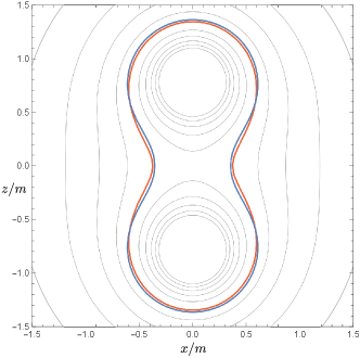
The reason why the value of is so small is that the electric field is approximately perpendicular to the marginally DTTS. From the formula for given in Eq. (44), this means that the marginally DTTS approximately coincides with a contour surface of . Figure 3 confirms this feature for . Here, the blue curve depicts the marginally DTTS, and the red curve shows the contour surface of . They agree well.
The lesson from this numerical experiment is that if a spacetime is static, the quantity is small and does not play an important role in the Penrose-like inequality for a DTTS. Of course, it is expected that the absolute value of may become large if dynamical situations are considered. For example, if two black holes have opposite charges, the contribution of the electric pressure would become important, although such a situation is more difficult to study. Exploring such issues is left as a remaining problem.
6 Summary and discussion
In this paper, we have examined the properties of LTSs and DTTSs for Einstein-Maxwell systems, particularly focusing on the derivation of Penrose-like inequalities on their area. Similarly to the Riemannian Penrose inequality for charged cases, the electric charge comes into the inequalities, but there are additional contributions from the density or the pressure/tension of electromagnetic fields in general. This is a rather interesting result because one naively expects that the upper bound for the area of an LTS and a DTTS is that of the photon sphere , where is the radius of an unstable circular orbit of a photon in the Reissner-Nordström spacetime given in Eq. (10). For an LTS, we have a tighter inequality than the naive one. For a DTTS, the obtained inequality can become both stronger and weaker depending on the configuration of electromagnetic fields. We have numerically examined the value of the correction term, represented by in Eq. (32), for a Majumdar-Papapetrou two-black-hole spacetime. Although the correction term makes the inequality weaker, we have checked that the value of is very small in that situation.
Up to now, we have assumed that the magnetic charge vanishes. Here, we consider what happens to our inequalities when nonzero is present. We first consider the case of an LTS. Since the total squared charge appears in the metric of the Reissner-Nordström solution when both the electric and magnetic fields are present, we would like to present the Penrose-like inequality in terms of . For this reason, we have to use the inequality
| (46) |
in the calculations of Eqs. (16) and (17). As a result, we must introduce the quantity
| (47) |
instead of of Eq. (14). The resultant inequality is the one of Eq. (13) but being replaced by . Next, we consider the case of a DTTS. Similarly to the case of an LTS, we must use the inequality of Eq. (46) (but being replaced by ) in the calculations of Eqs. (34) and (35). As a result, instead of , we must introduce . The resultant inequality is the same as the one of Eq. (31), but being replaced by . These results are summarized as follows:
Corollary 1.
In the main article of this paper, we have not considered a TTS for the static and stationary spacetimes defined in our previous paper Yoshino:2017 . We note that the concepts of a TTS and a DTTS are related but independent of each other in the sense that no inclusion relationship can be found Yoshino:2020-1 . In Appendix A, we present a theorem on the Penrose-like inequality for a TTS in a static spacetime, which is very similar to Theorem 2.
Throughout this study, we have not used the property of Maxwell’s equations except for Gauss’ law. The information from Maxwell’s equation may further restrict the properties of LTSs, DTTSs, and TTSs, especially for static/stationary spacetimes with static/stationary electromagnetic fields.
T. S. and K. I. are supported by Grant-Aid for Scientific Research from Ministry of Education, Science, Sports and Culture of Japan (No. 17H01091). H.Y. is supported by the Grant-in-Aid for Scientific Research (C) (No. JP18K03654) from Japan Society for the Promotion of Science (JSPS). The work of H.Y. is partly supported by Osaka City University Advanced Mathematical Institute (MEXT Joint Usage/Research Center on Mathematics and Theoretical Physics).
Appendix A Transversely trapping surface
The four of the present authors also proposed the concept of a TTS Yoshino:2017 . This concept is applicable only to static or stationary spacetimes. The definition is as follows :
Definition 3.
A static/stationary timelike hypersurface is a transversely trapping surface (TTS) if and only if arbitrary light rays emitted in arbitrary tangential directions of from arbitrary points of propagate on or toward the inside region of .
The necessary and sufficient condition for a surface to be a TTS (the TTS condition hereafter) is expressed as , where is the extrinsic curvature of and are arbitrary null vectors tangent to . For a static spacetime, there is the Killing time coordinate whose basis vector is orthogonal to the hypersurface, denoted by . The lapse function is defined by , where is a future-directed unit normal to . We denote the two-dimensional section of and by . As shown in Eq. (15) of Ref. Yoshino:2017 , the TTS condition is reexpressed in terms of as
| (48) |
where is the largest value among the two eigenvalues of the extrinsic curvature of in , is a spacelike unit normal to , and is the covariant derivative with respect to . In this situation, it is possible to derive the relation
| (49) |
For a convex TTS, we can derive the inequality
| (50) |
These relations are presented as Eqs. (24) and (25) in Ref. Yoshino:2017 . We now consider the Einstein-Maxwell system. Using Eq. (8), we find
| (51) |
Compare this inequality with the one of Eq. (34). Integrating over , we obtain exactly the same inequality as the one of Eq. (35). Therefore, a TTS in a static spacetime satisfies the same inequality as the Penrose-like inequality for a DTTS in time-symmetric initial data. This result is summarized as the following theorem:
Theorem 3.
As remarked in the final section, this theorem applies to the case that the magnetic charge is zero. When is nonzero, must be replaced by , where is given in Eq. (47).
References
- (1) C. M. Claudel, K. S. Virbhadra and G. F. R. Ellis, J. Math. Phys. 42, 818 (2001). [gr-qc/0005050].
- (2) H. Yoshino, Phys. Rev. D 95, 044047 (2017) [arXiv:1607.07133 [gr-qc]].
- (3) V. Cardoso, A. S. Miranda, E. Berti, H. Witek and V. T. Zanchin, Phys. Rev. D 79, 064016 (2009) [arXiv:0812.1806 [hep-th]].
- (4) K. Akiyama et al. [Event Horizon Telescope Collaboration], Astrophys. J. 875, L1 (2019) [arXiv:1906.11238 [astro-ph.GA]].
- (5) K. S. Virbhadra and G. F. R. Ellis, Phys. Rev. D 62, 084003 (2000). [astro-ph/9904193].
- (6) T. Shiromizu, Y. Tomikawa, K. Izumi and H. Yoshino, Prog. Theor. Exp. Phys. 2017, 033E01 (2017) [arXiv:1701.00564 [gr-qc]].
- (7) H. Yoshino, K. Izumi, T. Shiromizu and Y. Tomikawa, Prog. Theor. Exp. Phys. 2017, 063E01 (2017) [arXiv:1704.04637 [gr-qc]].
- (8) H. Yoshino, K. Izumi, T. Shiromizu and Y. Tomikawa, Prog. Theor. Exp. Phys. 2020 023E02 (2020) [arXiv:1909.08420 [gr-qc]].
- (9) H. Yoshino, K. Izumi, T. Shiromizu and Y. Tomikawa, Prog. Theor. Exp. Phys. 2020 053E01 (2020) [arXiv:1911.09893 [gr-qc]].
- (10) D. V. Gal’tsov and K. V. Kobialko, Phys. Rev. D 99, 084043 (2019) [arXiv:1901.02785 [gr-qc]].
- (11) R. Penrose, Annals N. Y. Acad. Sci. 224, 125 (1973).
- (12) S. Hod, Phys. Lett. B 727, 345-348 (2013). [arXiv:1701.06587 [gr-qc]].
- (13) P. S. Jang, Phys. Rev. D 20, 834 (1979).
- (14) R. Geroch, Ann. N. Y. Acad. Sci. 224, 108 (1973).
- (15) P. S. Jang and R. M. Wald, J. Math. Phys. 18, 41 (1977).
- (16) G. Weinstein and S. Yamada, Commun. Math. Phys. 257, 703-723 (2005) [arXiv:math/0405602 [math.DG]].
- (17) M. Khuri, G. Weinstein and S. Yamada, Contemp. Math. 653, 219-226 (2015) [arXiv:1308.3771 [gr-qc]].
- (18) M. Khuri, G. Weinstein and S. Yamada, J. Diff. Geom. 106, no.3, 451-498 (2017) [arXiv:1409.3271 [gr-qc]].