Loop Shaping of Hybrid Motion Control with Contact Transition
Abstract
A standard (stiff) motion control with output displacement feedback cannot handle unforeseen contact with environment without penetrating into soft, i.e. viscoelastic, materials or even damaging brittle or fragile materials. Robotics and mechatronics with tactile and haptic capabilities, and medical assistance systems in particular, place special demands on the advanced motion control systems that should enable safe and harmless contact transitions. This paper demonstrates how the fundamental principles of loop shaping can easily be used to handle the sufficiently stiff motion control with a sensor-free dynamic extension to reconfigure at contact with environment. Hybrid control scheme is proposed. Remarkable feature of the developed approach is that no measurement of the contact force is required and the input signal and measured output displacement are the only quantities used for control design and operation. Experimental scenarios for 1-DOF actuator are shown where the moving tool comes into contact with grape fruits that are soft and penetrable at the same time.
I Introduction
Motion control systems that can come in a well specified or (more importantly) unforseen contact with environmental objects have always been the focus of active research, especially in the field of control and robotics, starting already in the eighties of the last century. For instance, dynamics stability issues during contact with stiff environments were recognized and addressed (often in context of industrial robotics), see [1], when a manipulator in the force control mode comes in touch with a stiff and kinematically constrained environmental object. A milestone was the introduction of the concept of impedance control [2] and later of hybrid impedance control [3], which enabled a deep understanding of the most important (i.e., physically justifiable) interactions and limitations for the controlled impedance–admittance pair of a mechanical motion system in contact with its environment. Motion control of an unconstrained manipulation, on the one hand, and force control of a constrained interaction between the manipulator and its environment, on the other hand, became quickly to ’stumbling block’, especially in view of controlling contact transitions, see e.g. discission with experiments in [4]. For a former brief survey of the force control of manipulators we refer to e.g. [5], while a more recent overview of the force control can be found in the literature like e.g. Springer Handbook of Robotics [6].
The ideas of impedance and admittance control of robotic manipulators, [2, 3], found quickly a way and appreciation in motion control for drives and mechatronic systems [7]. A unified passivity-based control framework for position, torque and impedance control, which use the full state feedback and a dedicated energy shaping with variable gain strategy was also proposed in [8]. Another focus on decomposing (correspondingly switching) the control structure led to hybrid position/force controllers, the first one proposed (most probably) in [9]. A widely adopted strategy of hybrid force/motion control, which aims at controlling the motion along the unconstrained task directions and force along the constrained task directions, is using a certain decomposition which allows simultaneous control of both the contact force and the end-effector motion in two mutually independent subspaces, see [6] for details. Here, a selection strategy for the stiffness/compliance parameters and the desired and feedback variables must be part of the overall control law and is known to be non-trivial and fundamental to the specification of the control task. Although impedance modulation and reconfiguration (corresponding switching) are widely used in hybrid position/force control in robotics, see e.g. [10], equally as in other motion control systems such as hydraulic actuators [11], the problems of transition and stability of structural switching [12] remain among the most relevant. It should be emphasized that during a contact transition, both a hybrid position/force control and the process plant itself undergo a structural change. For sufficiently damped contact transitions and relatively slow dynamics of some available internal state variable experiencing a threshold value upon the contact, a hysteresis relay-based switching policy can be developed, see e.g. [13]. For combining the robustness property of impedance control in stiff contact with the accuracy of admittance control in soft contact various approaches were proposed in robotics. For instance, a predictive instantaneous model impedance control scheme was described in [14], and continuous switching (with duty cycle as design parameter) between controllers with impedance and admittance causality was provided, also with experiments, in [15].
An important causality constraint is that no one motion system can simultaneously impress a force on its environment and impose a displacement or velocity on it. Only one of both control variables, either interaction force or relative motion of the environmental object, can be determined along each degree of freedom [2]. This results from an instantaneous power flow between two or more physical systems. Recall that the power flow is definable as product of an effort and a flow variable, force and velocity for mechanical systems, respectively. Given these basic principles, it seems obvious that different control concepts and an approach for combining them are required to control unconstrained and constrained motion and the resulting contact force.
A frequently appearing question is nevertheless how to handle those manipulator-environment configurations where a control design is a priori constrained by some given structure, the application specification and, most importantly, by the sensors and their arrangement.
In this work, an intuitively understandable (for standard motion control design in frequency domain) approach of reshaping the otherwise stiffly designed feedback controllers is proposed. This way, a smooth and stable contact transition can be guaranteed without applying a more complex control structure. Most importantly, only the measured output displacement is used for feedback and the designed hybrid motion control does not require additional force sensors or observers of internal states. The rest of the paper is organized as follows. In section II we discuss the types of impedance operators that represent an interaction with the environment and relate them to the control loop properties required for a contact transition. Section III introduces the thereupon based hybrid motion control design. A detailed experimental case study with soft but penetrable grape objects coming into contact with the mechanical tool which is driven by the displacement feedback control is demonstrated in section IV. Brief conclusions are drawn in section V.
II Impedance and shaping of disturbance sensitivity function
For motion control at large, with one relative degree of freedom in the generalized coordinates, one can define the control stiffness, cf. [7], [16], as
| (1) |
Here is the overall net force (in the generalized coordinates) imposed on the moving body of the motion control system under consideration. For a matched disturbance force and a feedback control value , which inherently has dimension of a force in motion control, the total net force can be considered as a superposition . Indeed, when a generic motion control system
| (2) |
with the sufficiently smooth flow map and the vector of states variables (often with and as a vector of relative displacement and velocity) is in steady-state, the control should balance the counteracting disturbance. Let us fix next some controlled operation point, in terms of , and consider this way reduced (1) in Laplace domain. Then, one can write
| (3) |
provided that the Laplace transform of the control stiffness operator exists. Also we note that an equivalence between and is valid only for low frequency range, cf. [3]. Recalling that for a linear environment, the impedance is defined as the ratio of the Laplace transforms of effort and flow [17], the mechanical impedance is written as:
| (4) |
that leads to a generic relationship
| (5) |
Since a dynamic interaction between two physical bodies implies that one must complement the other, i.e. along any degree for freedom if one is an impedance, the other must be admittance and vice versa, see [2], the condition (5) becomes crucial. It reveals how the motion control system can be designed when an environment is classified by .
Using the mechanical impedance definition (4), one can classify the following (typical) contact environments, which are associated with the corresponding impedance operators. The first one is the viscous dashpot, shown schematically in Fig. LABEL:fig:environm (a).
The constitutive equation of the Newtonian fluid in a dashpot, i.e. where is viscosity, results in , meaning the contact environment is resistive, cf. [17]. If one expects the environment to be viscoelastic, i.e. to exhibit also a certain capacitive behavior, then one can assume a Kelvin-Voigt contact, that is schematically shown in Fig. LABEL:fig:environm (b). This leads to the corresponding impedance operator . Note that for modeling the environmental impedance, more complex structures than those shown in Fig. LABEL:fig:environm can equally be assumed, and even variable and nonlinear structures might be considered. This would, however, go far beyond the scope of this work, and it turns out to be superfluous for a straightforward design of linear and hybrid motion controllers.
Now, consider the loop transfer function
| (6) |
of the motion control system with the input-output plant and feedback controller which receives the control error as input. Obviously, the control reference command conforms to some application-related specifications, before and after a possible contact with environment and without it. While the reference-to-output transfer function can be determined by shaping , correspondingly designing to be possibly stiff, i.e. having possibly high bandwidth of and possibly unity for all angular frequencies , we focus in the following on the disturbance response to . The disturbance-to-output transfer characteristics are given by
| (7) |
and often denoted and disturbance sensitivity function, cf. e.g. [18]. While an ideal position (or velocity) controller should not allow any steady-state or transient deviations for any force imposition on mechanical system, i.e. the controller stiffness should be infinite, cf. [7], a hybrid motion controller with contact transition should allow to match the properties of the contact with environment. Comparing (3), (5), and (7) one can recognize that
| (8) |
To further interpret the results obtained above, it is worth recalling a fundamental distinction between a mechanical admittance and impedance [2]. Multiple physical systems can be described in one form but not in the other. For instance, elastic contacts approximated by a non-monotonic constitutive equation can only be seen as impedance, i.e. , but not as admittance. Indeed, prior to a mechanical contact is established, the map is not given. Similar issue appears in case of a tangential kinetic friction force, cf. [19]. Nevertheless, the admittance of the motion control, which is equivalent to disturbance sensitivity function (7), can certainly be used at the same moment as the mechanical contact with environment arises. This will be discussed and used further below in the derivation of hybrid motion control.
III Hybrid motion control
First, we proceed with designing a (sufficiently) stiff feedback motion control, denoted by . Following the most simple loop shaping methodology and assuming the critically damped dominant pole pair of the closed-loop system, the reference-to-output transfer function yields
| (9) |
Here the control specification is given by only the natural frequency (approximately to bandwidth) of the closed-loop. Recall that higher values imply higher stiffness of the controlled system. Using the given system transfer function and applying the block diagram algebra, the resulting motion control is
| (10) |
Note that for system plants with a relative degree , the control (10) yields a proper transfer function and, thus, can be directly implemented.
Now, for designing an impedance controller, assume a sensitivity function, cf. (8),
| (11) |
that corresponds to a viscous (dashpot-type) contact with environment, cf. section II. Using (7) and the block diagram algebra, the resulting impedance controller, denoted as viscous , is determined by
| (12) |
Note that (12) reveals an improper transfer function so that an additional low-pass filter with a sufficiently high cut-off frequency needs to applied in series with .
The magnitude response of , , , and transfer functions are depicted in Fig. 2 for the exemplary assumed system plant with two negative real poles at , and the design parameters and . Note that both disturbance sensitivity functions are determined according to (7) for each of the feedback controllers and .
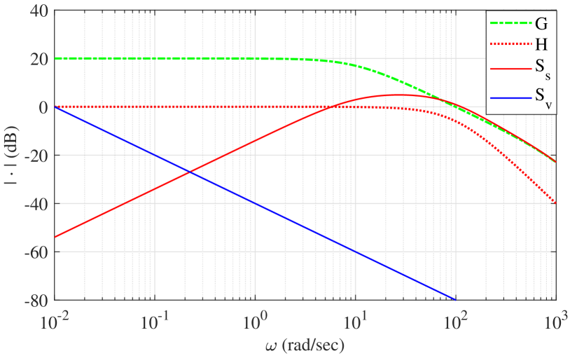
It is easy to interpret from the Bode plot of that a step-wise disturbance , which appears at the contact instant, will be largely suppressed by the stiff motion control. Following to that, the controlled mechanical motion system will penetrate into the environmental object or moves it away from itself if the latter is unconstrained. Quite the opposite, the viscous impedance control will react to the step-wise contact force by inducing a repulsive relative displacement in the opposite direction. Here it is worth noting that since it leads to release of the contact, the disturbance becomes zero and the relative motion will stop, cf. below with the experimental results.
Recall that for achieving stable and smooth contact transitions, a general strategy of the motion control is to regulate the system displacement and/or velocity (as conventional manipulators do) and provide additionally a well-specified disturbance response for deviations from this motion. According to [2], such disturbance response has the form of an impedance, that may be then modulated and adapted depending on the control tasks and environment. Despite such straightforward impedance paradigm, that gives the name ’impedance control’ [2], one task that is not always solvable remains the detection of contact, correspondingly recognition of the associated deviations from a well-specified (i.e. nominal) motion. Mostly, the contact forces are measured by a force sensor connected to the wrist of manipulator or integrated in the front-end tool. The use of internal (i.e. not only output displacement) measurements or even external senors can be found both in the theoretical works, cf. e.g. [20] and experimental studies in robotics, e.g. [21, 10].
If the controlled output displacement is the only measurable state of the motion system (the case we consider in this work), the control reshaping can be triggered exclusively by an information content of the control signal. Assuming some nominal bound of the control signal , that is mostly possible for the given nominal plant , control , and reference , an overshot will indicate appearance of the disturbance force . Note that this strategy can be used in particular when the stiff motion controller contains an integral control action. Indeed, during a compensated steady-state motion, an exceeded control force is proportional to an additional disturbing force. Since a dynamic transition from to should not provoke any undesired transients in direction of the contact with environment, it is worth examining the disturbance-to-control-value transfer characteristics which are given by . For both controllers (10) and (12), as exemplary designed above, this is shown by the magnitude response in Fig. 3.
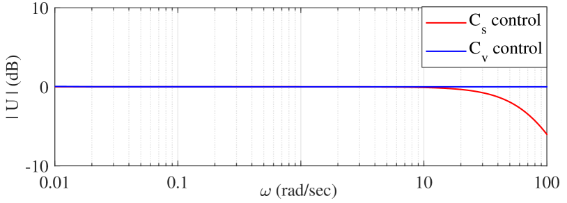
One can recognize that since is set to zero for , and the control magnitude response of both and have nearly the same value, an appearance of the step-wise disturbance at will lead to a decrease of by the magnitude equal to for . The force imposed on the environmental object under contact drops respectively.
IV Experimental case study
IV-A Motion system and contact scenarios
In the following, we demonstrate an experimental case study of the proposed hybrid motion control with the smooth transition when the moving tool experiences unforeseen contact with environment. The latter is soft yet penetrable, emulating one of the most critical applications of motion control – robotic assistance for medical diagnosis and surgery. For that purpose, a half of the grape is placed in way of the moving mechanical tool, see Fig. LABEL:fig:expsetup, which is controlled by using only the displacement feedback. The relative displacement of the tip of the tool is sensed remotely, i.e. contactless, cf. Fig. LABEL:fig:expsetup. Note that the way how the vertical displacement is measured provides a relatively high level of the noise and, thus, represents rather a worst case scenario for the control application. The system input and output (in volt) and (in meter), respectively, are the only quantities available for the control design and operation.
The experimental motion system in actuated by a voice-coil-motor and has one translational degree of freedom. The rigid mechanical tool is moving in vertical direction and has a relatively low displacement range about 0.015 m. The implemented feedback control is running on the dedicated real-time board with the set sampling rate of 10 kHz. For more technical details, including the physical system parameters, an interested reader is referred to [22].
The nominal system model is given by
| (13) |
where is Laplace variable, and and are the known system gain and time-constant parameters, respectively. The constant term constitutes the nominal disturbance due to the gravity force which is known. Therefore, the latter is pre-compensated, so that the system input signal results in
where the feedback controller output is designed as described in section III.
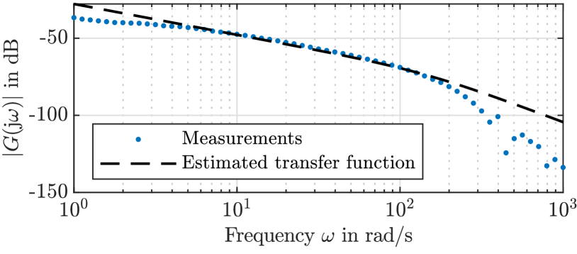
Due to a free integrator, cf. (13), the identification of the free system parameters was performed in a closed-loop configuration, see [23] for details. The least-squares determined parameter values are and sec, while the experimentally measured and identified magnitude response are shown towards each other in Bode diagram in Fig. 5.
Note that an additional electrical time constant of the voice-coil-motor dynamics, which is about sec, is not explicitly taken into account, equally as not a minor time delay in the input-output loop of the system. Both are neglected in the nominal model (13), cf. [23]. At the same time, they constitute an additional robustness criterion for the motion control system under evaluation and, this way, contribute to a worst-case scenario of the study.
IV-B Evaluated motion control
For a sufficiently stiff motion control, i.e. the one without contact transition and featuring , a standard PID (proportional-integral-derivative) controller
| (14) |
is assumed. The controller transfer function is considered as ’stiff’ and denoted by . The applied robust design procedure, provided in [23], rests on an underlying PD control with a stable pole-zero cancelation (i.e. canceling the plant time constant ) and an upper bound of the disturbance sensitivity function. The determined this way control parameters are , , and .
Two reshaped ’soft’ feedback controllers which allow for a stable and smooth contact transition are designed, cf. section II. The first one, denoted by , is to enable a purely viscous and well damped repulsive behavior when contacting with environment, and it yields
| (15) |
Another reshaped feedback controller, denoted by , is more ’stiff’ and enables for a viscoelastic behavior when contacting with environment, cf. section II. The resulting controller has the form
| (16) |
similar to (15) but differs from this by including also the proportional feedback of the control error, cf. with (14). The latter makes it possible to press on the environment with a force that is either proportional to the control error (in which case the reference value is to be considered additionally), or with a constant force equal to . For the second case, which is also used in the below experiments, the proportional control part in (16) is extended by saturation, i.e. . Further we note that both fractions in (15) and (16) use a low-pass filter with a sufficiently high cut-off frequency ; otherwise both control transfer functions are improper and could not be implemented, cf. section III.
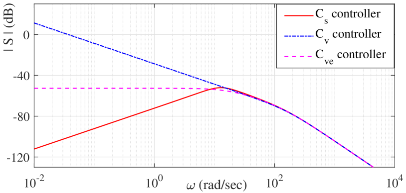
The resulted magnitude response of the closed-loop disturbance sensitivity function is compared for all three feedback controllers (here for ) in Fig. 6.
The experimentally evaluated motion control scenario is shown in Fig. 7 (a). The reference trajectory with one positive and one negative slope, both implying the same reference velocity magnitude, is tracked by the designed stiff controller (14). On the way back, i.e. at time sec, there is no environmental obstacles and, therefore, no contact with soft objects, cf. with Fig. LABEL:fig:expsetup where a soft object was already placed. Note that at the beginning and especially after the slope segments of trajectory, the control error increases and takes certain time to settle, cf. Fig. 7 (a). This is due to nonlinear friction effects (see [19] for details) which are not explicitly compensated and need to be mitigated by the proportional and integral feedback actions only.
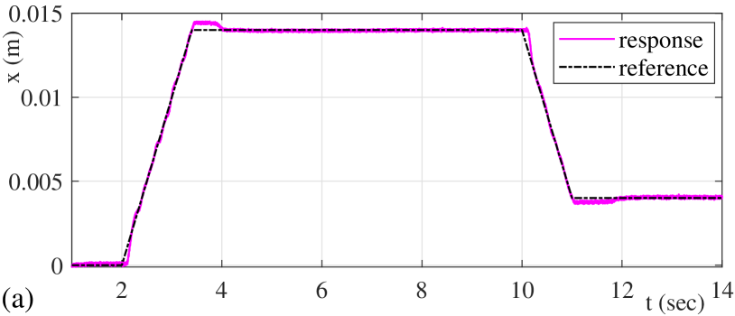
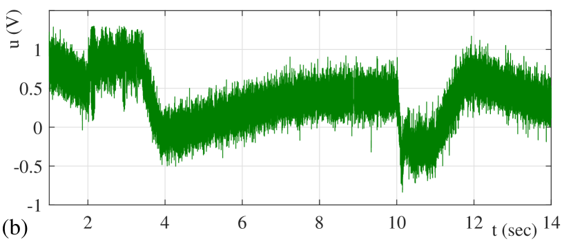
The output of the feedback controller is depicted in Fig. 7 (b), indicating that it stays in a certain bound. The control reshaping threshold is set to . Recall that once , the feedback control changes from its stiff configuration, i.e. (14), to a compliant one, i.e. either (15) or (16) as both controllers and were evaluated. Also recall that the reshaping threshold value corresponds to the disturbance force which increases more the stiff motion controller is loading the contacting object, cf. section II.
Following to that, the experimental scenarios with a soft environmental object, which is a half of the grape placed before the way back i.e. at time sec, were evaluated. The final state is exemplified in Fig. LABEL:fig:expsetup. Three control configurations were evaluated. The first one is the stiff control (14) without hybrid reconfiguration to a compliant controller. The second is the stiff control (14) which is reconfigured into the viscous control (15) upon the reshaping threshold . Finally the third is the stiff control (14) which is reconfigured into the viscoelastic control (16) upon the reshaping threshold . Recall that the viscoelastic control (16) is additionally subject to saturation at since it contains also feedback proportional to the displacement error .
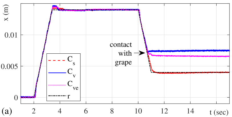
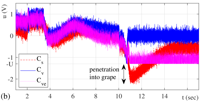
The measured displacement response and the feedback control value are shown in Fig. 8 (a) and (b), respectively. One can recognize that the stiff control reaches the back reference position (for sec), thus ploughing the mechanical tool into the soft environment, cf. Fig. LABEL:fig:expsetup (a). Its control value falls below the set threshold and represents the corresponding force required to penetrate into the grape. Quite the opposite, the viscous control , activated by exceeding the threshold value, provides a slightly repulsive response which can be associated with certain elasticity of the grape surface, cf. Fig. LABEL:fig:expsetup (b). The controller maintains the contact position while the control value has a zero mean and almost the same high frequency pattern as the control; this is due to the sensor noise and the corresponding output derivative. A slightly differing behavior can be seen in case of the viscoelastic controller . Due to a sufficiently large control error for sec and, at the same time, the used control saturation in , the motion system does not penetrate into the grape, but presses it further with the corresponding threshold magnitude. Here we recall that at steady-state, the control value is proportional to the disturbance force coming from the environment.
V Conclusions
In this communication, we provided an easy interpretable (in frequency domain) analysis and design of dynamic reshaping of the stiff (admittance) motion control to a soft (impedance) control upon the contact with constrained and deformable environmental objects. Only the measured output displacement in feedback is used for the overall control design and operation. Hybrid control scheme was established and revealing control experiments with contacting the soft but penetrable objects, i.e. grape, were provided.
References
- [1] C. An and J. Hollerbach, “Dynamic stability issues in force control of manipulators,” in American Control Conference, 1987, pp. 821–827.
- [2] N. Hogan, “Impedance control: An approach to manipulation: Part I – theory,” Transactions of the ASME, vol. 107, no. 1, pp. 1–7, 1985.
- [3] R. Anderson and M. Spong, “Hybrid impedance control of robotic manipulators,” IEEE Journal on Robotics and Automation, vol. 4, no. 5, pp. 549–556, 1988.
- [4] J. Hyde and M. Cutkosky, “Controlling contact transition,” IEEE Control Systems Magazine, vol. 14, no. 1, pp. 25–30, 1994.
- [5] T. Yoshikawa, “Force control of robot manipulators,” in IEEE International Conference on Robotics and Automation, 2000, pp. 220–226.
- [6] L. Villani and J. De Schutter, “Force control,” in Springer Handbook of Robotics, pp. 195–220, 2016.
- [7] K. Ohnishi, N. Matsui, and Y. Hori, “Estimation, identification, and sensorless control in motion control system,” Proceedings of the IEEE, vol. 82, no. 8, pp. 1253–1265, 1994.
- [8] A. Albu-Schäffer, C. Ott, and G. Hirzinger, “A unified passivity-based control framework for position, torque and impedance control of flexible joint robots,” The International Journal of Robotics Research, vol. 26, no. 1, pp. 23–39, 2007.
- [9] M. Raibert and J. Craig, “Hybrid position/force control of manipulators,” ASME Journal of Dynamic Systems, Measurement, and Control, vol. 103, no. 2, pp. 126–133, 1981.
- [10] F. Ficuciello, L. Villani, and B. Siciliano, “Variable impedance control of redundant manipulators for intuitive human–robot physical interaction,” IEEE Tran. on Robotics, vol. 31, no. 4, pp. 850–863, 2015.
- [11] P. Pasolli and M. Ruderman, “Hybrid position/force control for hydraulic actuators,” in IEEE 28th Mediterranean Conference on Control and Automation (MED), 2020, pp. 73–78.
- [12] D. Liberzon and A. S. Morse, “Basic problems in stability and design of switched systems,” IEEE Control Systems Magazine, vol. 19, pp. 59–70, 1999.
- [13] M. Ruderman, “On switching between motion and force control,” in IEEE 27th Mediterranean Conference on Control and Automation (MED), 2019, pp. 445–450.
- [14] T. Valency and M. Zacksenhouse, “Accuracy/robustness dilemma in impedance control,” ASME Journal of dynamic systems, measurement, and control, vol. 125, no. 3, pp. 310–319, 2003.
- [15] C. Ott, R. Mukherjee, and Y. Nakamura, “A hybrid system framework for unified impedance and admittance control,” Journal of Intelligent & Robotic Systems, vol. 78, pp. 359–375, 2015.
- [16] M. Ruderman, M. Iwasaki, and W.-H. Chen, “Motion-control techniques of today and tomorrow: a review and discussion of the challenges of controlled motion,” IEEE Industrial Electronics Magazine, vol. 14, no. 1, pp. 41–55, 2020.
- [17] M. Spong, S. Hutchinson, and M. Vidyasagar, Robot Modeling and Control. John Wiley & Sons, 2005.
- [18] K. J. Åström and R. Murray, Feedback systems: an introduction for scientists and engineers. Princeton University Press, 2021.
- [19] M. Ruderman, Analysis and compensation of kinetic friction in robotic and mechatronic control systems. CRC Press, 2023.
- [20] C. P. Bechlioulis, Z. Doulgeri, and G. A. Rovithakis, “Guaranteeing prescribed performance and contact maintenance via an approximation free robot force/position controller,” Automatica, vol. 48, no. 2, pp. 360–365, 2012.
- [21] A. De Luca, A. Albu-Schaffer, S. Haddadin, and G. Hirzinger, “Collision detection and safe reaction with the DLR-III lightweight manipulator arm,” in 2006 IEEE/RSJ International Conference on Intelligent Robots and Systems, 2006, pp. 1623–1630.
- [22] M. Ruderman, “Motion control with optimal nonlinear damping: from theory to experiment,” Control Engineering Practice, vol. 127, p. 105310, 2022.
- [23] M. Ruderman, J. Reger, B. Calmbach, and L. Fridman, “Disturbance sensitivity analysis and experimental evaluation of continuous sliding mode control,” arXiv preprint arXiv:2208.06608, 2022.