Loop Quantum Photonic Chip for Coherent Multi-Time-Step Evolution
Abstract
Quantum evolution is crucial for the understanding of complex quantum systems. However, current implementations of time evolution on quantum photonic platforms face challenges of limited light source efficiency due to propagation loss and merely single-layer complexity. In this work, we present a loop quantum photonic chip (Loop-QPC) designed to efficiently simulate quantum dynamics over multiple time steps in a single chip. Our approach employs a recirculating loop structure to reuse computational resources and eliminate the need for multiple quantum tomography steps or chip reconfigurations. We experimentally demonstrate the dynamics of the spin-boson model on a low-loss Silicon Nitride (SiN) integrated photonic chip. The Loop-QPC achieves a three-step unitary evolution closely matching the theoretical predictions. These results establish the Loop-QPC as a promising method for efficient and scalable quantum simulation, advancing the development of quantum simulation on programmable photonic circuits.
I Introduction
Simulating the evolution of quantum systems [1, 2] represents one of the most promising applications of programmable quantum processors [3, 4], providing practical means to explore and understand complex quantum systems that remain intractable for classical computers. A notable testbed for studying complex quantum evolution is the spin-boson model [5, 6] that describes the dynamics of a spin coupled to a bath. This model plays a crucial role in understanding light-matter interactions [7], quantum chemistry [8], charge transfer [9], exciton transport [10], macroscopic quantum tunneling in superconducting systems [11], polarons [12], and the nonadiabatic dynamics of molecules [13].
Recently, there has been significant progress in the development of different quantum processor platforms, including ultracold gases [14], trapped ions [15], superconducting qubits [16], and photonic [17, 18], even for the simulation of spin-boson-like systems [19, 20, 21]. The development of photonic systems has led to the introduction of on-chip quantum processors with the integration of photon generation and detection. These photonic chips [22, 22, 23, 24] are solid state solutions, which work at room temperature, are reprogrammable, and whose realization is compatible with existing semiconductor fabrication technology. Importantly, they can be used for fault-tolerant computing, variational approaches, and analogue quantum simulation [25].
However, implementing quantum evolution on photonic platforms still presents significant challenges. Current approaches primarily rely on sequentially modifying chip parameters to perform time evolution for different time durations [26]. Additionally, these methods require reloading the computed unitary parameters [27, 28] or input states [22] onto the chip at each time step, resulting in significant overhead from repeated digital-to-analog and analog-to-digital conversions, as well as increased computational costs for recalculating the unitary parameters. To address these issues, multiplexing techniques such as wavelength-division multiplexing [29] and time-division multiplexing [30] have been explored. However, while these approaches can alleviate some hardware constraints, they often introduce additional challenges, including increased chip size and system noise. Furthermore, they do not eliminate the need for repeated quantum state tomography measurements, or repeated re-encoding of the output signal into a new input signal for the photonic chip.
To overcome these limitations, we propose a loop quantum photonic chip (Loop-QPC) that enables efficient quantum evolution by reusing a single chip for multiple time steps. The core of our design lies in a recirculating loop structure, which directs the output from one time step back into the system as input for the subsequent step, thereby eliminating the need for quantum state tomography and repeated parameter configurations. We thus program our Loop-QPC to execute the quantum evolution of the spin-boson model for time step . By leveraging the low-loss properties of Silicon Nitride (SiN) and the high detection efficiency of Superconducting Nanowire Single Photon Detectors (SNSPDs), we are able to use our photonic chip to simulate the quantum evolution for three distinct time steps with high fidelity, while being able to take measurements at each of the time steps.
II Model
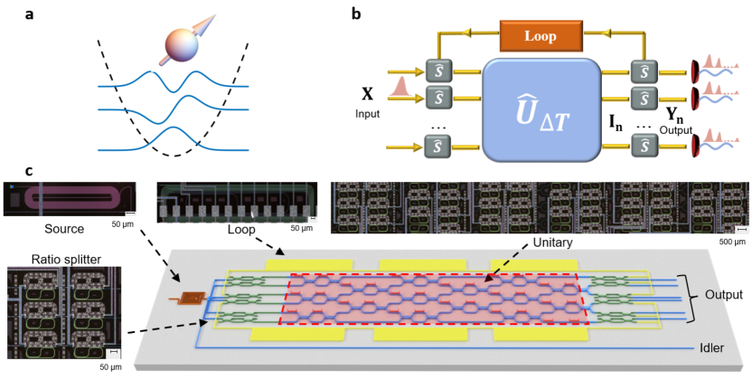
We consider the spin-boson model with a single spin coupled to a harmonic oscillator as depicted in Fig. 1a. In the strong coupling regime, its evolution in time is given by the following Hamiltonian [31],
| (1) |
where is Planck’s constant, and are the creation and annihilation operators for the harmonic oscillator, respectively, while the operators and are Pauli operators acting on the spin. The parameter represents the local magnetic field in the direction while is the field in the direction. The coupling strength between the spins and the harmonic oscillator is denoted by and is the frequency of the oscillator. In the following, we will consider two main regimes with fundamentally different dynamics. One in which the field, the coupling strength and the frequency are identical , and the case in which they are similar in magnitude but different in value, i.e. , so as to demonstrate the generalization of our setting.
To experimentally simulate the unitary time evolution generated by over a time , we decompose the evolution over time steps of duration and use
| (2) |
where is thus the evolution operator for a time .
III Loop-QPC Design
To represent the spin-boson model state and its evolution, we use the unary encoding (more detail on the unary encoding in App. A). In particular, we consider both levels for the spin and the first three levels for the harmonic oscillator, thus resulting in a total of 6 levels, one per channel of our photonic chip (similarly to [32]). Our design of the Loop-QPC, shown in Figs. 1b and c, is composed of seven main modules: the photon generation module that produces one photon for the computation and one idler photon, the data encoding module, the ratio splitter module, the quantum unitary computation module , the loop module , and the measurement module.
To facilitate the understanding of the process, we describe the system through three stages, input stage corresponding to the initial input in the Loop-QPC, intermediate stages that are the signal after going through the unitary portion times, and output stages that go to the measurement devices after passing times through the unitary. We use and for the two splitting ratios of the ratio splitters (derivation in App. D), where is the identity, indicates whether the ratio splitter is at the input () or output () of the unitary module, and we denote by the loop portion. We can thus write the evolution as
| (3) | ||||
For the experimental realization, we employ an integrated quantum photonic architecture implemented on a SiN chip as our experimental platform, as shown in Fig. 1c. This architecture minimizes the propagation path length and ensures uniform propagation loss across all paths. The structure consists of 15 unit cells. Each unit is constructed by a Mach-Zehnder interferometer (MZI) composed of two symmetric (50/50) beam splitters and an internal/external relative phase shift /. This configuration allows for the realization of an arbitrary 6-mode unitary matrix. The fundamental transformation of each unit cell is defined as,
| (4) |
Our compact phase shifter design shortens each MZI unit cell, effectively reducing the total propagation loss. Thanks to high-quality SiN fabrication, the waveguides achieve an optical transmission () around 0.6 dB/cm. The MZI architecture also facilitates the input/output ratio splitting. In the experiment, the initial values for and are computed first using Clements et al. decomposition [27] and further refined through machine learning techniques to enhance the fidelity. The detailed decomposition of the arbitrary -mode unitary matrix for the spin-boson model can be found in App. B, with machine learning optimization methods detailed in [33] and App. C. The loop module incorporates a low-loss SiN delay line in a spiral structure. This specially designed delay line ensures a fixed temporal separation between photons from adjacent loops, thereby preventing interference between different loop photons, which maintains the independence of the computations at each time step. To guarantee this independence, the loop length must exceed a critical threshold of cm computed from the speed of light in SiN and the temporal resolution of the SNSPD used for detecting photons. The low-loss SiN waveguides and high-efficiency SNSPDs are thus crucial for determining the large observable evolution steps in the Loop-QPC.
The whole Loop-QPC computing process is as follows: A pump laser operating at a 500 MHz repetition rate generates input light, resulting in signal peaks at 2 s intervals. The pump light initiates a pair of signal and idler photons in the long waveguide via the spontaneous four-wave mixing process. By regulating the pump power, we balance the photon generation rate and the probability of generating multi-pair terms. The signal photons are used for computation, while the idler photons are used as a heralding to mark the timing of the signal photon. Since the signal and idler photons are generated simultaneously, coincidence measurements enable precise determination of the arrival times of signal photons. Output photons are coupled to fibers through a grating array, and photon detection is performed using seven SNSPDs, with six dedicated to signal photons and one for idler photons. This configuration allows the Loop-QPC to collect multiple outputs from different loops on a single chip in a single run, thereby efficiently realizing quantum dynamic evolution.
IV Experimental Results
IV.1 Resolution of the time steps
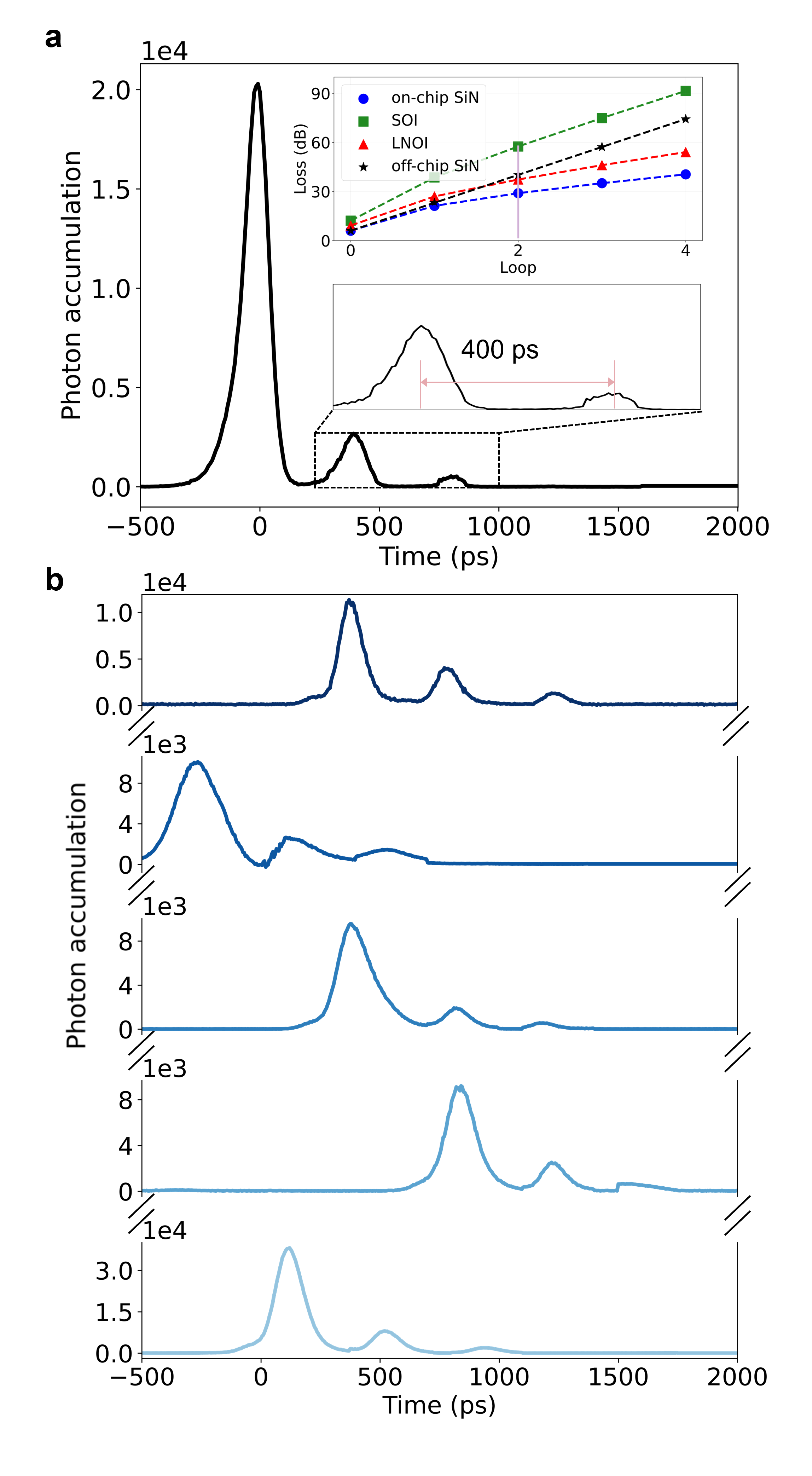
We first resolve three different intensity peaks in our setup. Running the experiment for a pair of signal and idler photons for 10 seconds produces the measured pair at a rate of photons per second. We record the time of arrival of signal photons in each of the channels, storing these times relative to the arrival time of their corresponding idler photon. In Fig. 2 we depict the count of photons per time and channel (from top to bottom from channel 1 to channel 6), showing a clear separation between three different arrival times, after going through the chip one, two, or three times. These peaks are well above the background noise and do not overlap, confirming the Loop-QPC ability to maintain clear signal separation. These results are obtained by programming the Loop-QPC such that the unitary module is derived from a trivial Hamiltonian described by an identity matrix.
To stress the advantages of the Loop-QPC we have designed, even for this trivial Hamiltonian, we numerically compare the photon losses versus the number of loops for different designs. We compare SOI platforms [23], LNOI platforms [34], and off-chip loop-based SiN setups [35]. In our loss calculations, we considered only the difference in transmission losses and functional units loss to each platform, with all other conditions remaining consistent with our platform. For the design with the off-chip loop case, we also account for the photons coupling loss during each loop. As shown in the inset of Fig. 2 a, our Loop-QPC design has reduced losses because it avoids some of the key issues of the other technologies, i.e. SOI platforms suffer from high propagation loop loss, LNOI platforms have high MZI propagation loss, and setups with off-chip loops experience high coupling loss for each loop. More details on the loss calculation comparisons and scalability for the Loop-QPC are provided in App. D and E, respectively.
IV.2 Evolution of Spin-Boson Model
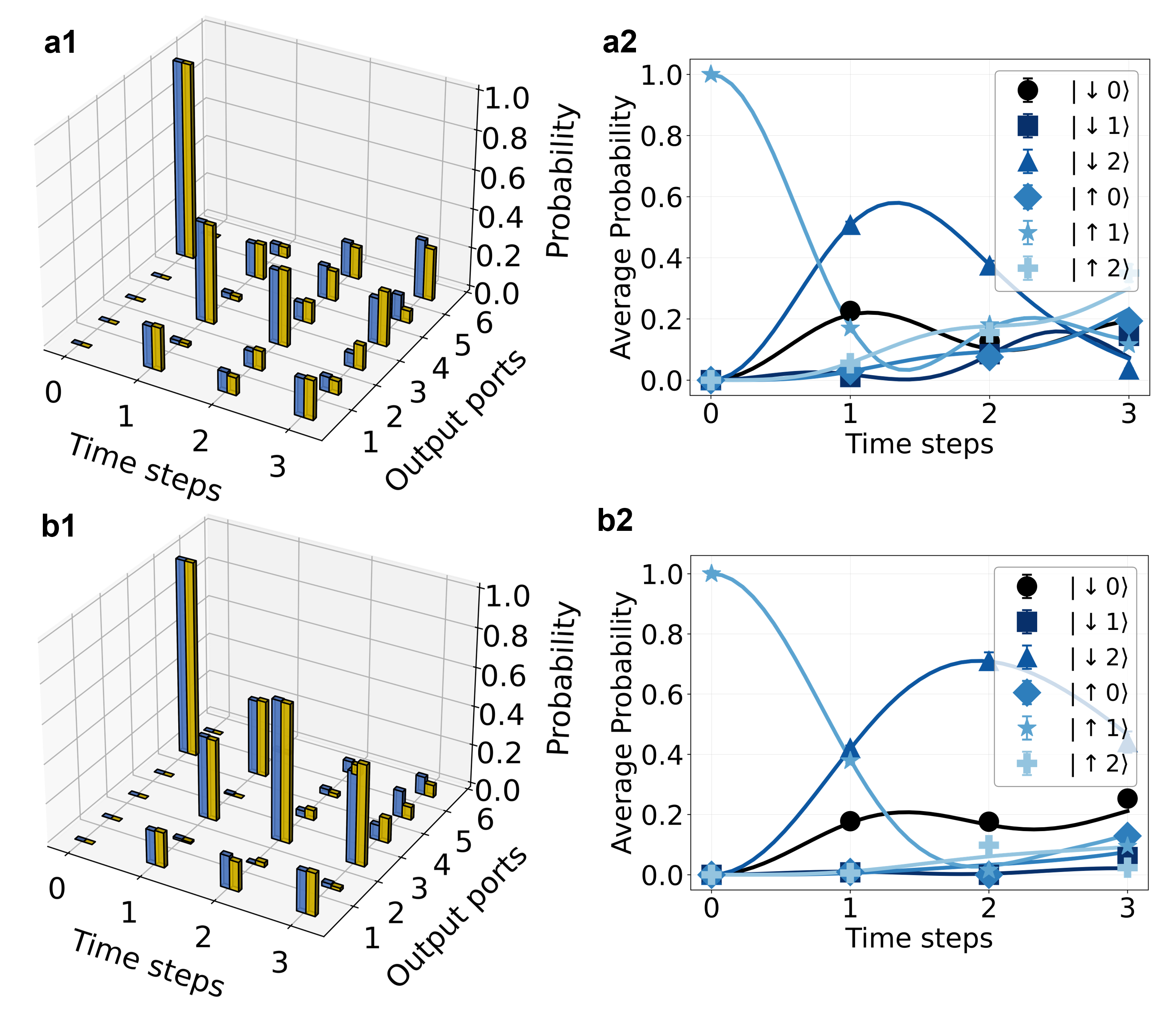
We now focus on the performance of our setup for the spin-boson model where, as the initial condition, we choose a pure product state between the spin and the bosons, where the spin is in the excited state and the harmonic oscillator has zero excitations. We choose two scenarios with and , , for which the different terms of the Hamiltonian are similarly in value. This setup can enable us to observe oscillatory and non-trivial dynamics without requiring a large number of levels of the harmonic oscillator.
The evolution of the system are simulated by the probability of measuring a photon in an exit channel at the different time steps and for two different sets of Hamiltonian parameters. Figure 3a present in a complementary manner the comparison between the experimental measurements and theoretical predictions at different time steps. For each set of parameters, we performed twenty sets of 10-second-long experiments and calculated both their average values and standard deviation in Fig. 3b. Overall, we observe a very good agreement with the theoretical predictions for both sets of parameters, despite the large difference in the probability of measuring a photon in the different channels. The error increases with the number of time steps, but it is however close to theoretical predictions.
V Conclusion
In this study, we have experimentally demonstrated the implementation of the unitary evolution operator for the Hamiltonian of the spin-boson model and its corresponding quantum dynamics on our Loop-QPC platform. The integrated design of a photonic circuit with loops, and the measurement method, allow us to simulate different time steps of the evolution with the same chip. This results in the avoidance of recalibrating the chip to simulate different time steps, or having to perform a state tomography to prepare states at intermediate times, which would require a significant amount of resources.
Furthermore, the approach is independent of the type of the unitary used nor of the encoding. It thus opens the way to the efficient, and scalable solution for quantum simulations, for example using binary encoding, advancing the potential of photonic quantum technologies. In the future, further reduction of the losses and improved tuning of the chip parameters could result in simulations for longer time steps and lower errors. This could open a way to simulate open dynamics by engineering, either via collisional models [36] or finite-size baths based on typicality [37].
References
- [1] Johnjoe McFadden. Quantum evolution. WW Norton & Company, 2002.
- [2] Mario Motta, Chong Sun, Adrian TK Tan, Matthew J O’Rourke, Erika Ye, Austin J Minnich, Fernando GSL Brandao, and Garnet Kin-Lic Chan. Determining eigenstates and thermal states on a quantum computer using quantum imaginary time evolution. Nature Physics, 16(2):205–210, 2020.
- [3] Andrew J Daley, Immanuel Bloch, Christian Kokail, Stuart Flannigan, Natalie Pearson, Matthias Troyer, and Peter Zoller. Practical quantum advantage in quantum simulation. Nature, 607(7920):667–676, 2022.
- [4] Suguru Endo, Jinzhao Sun, Ying Li, Simon C Benjamin, and Xiao Yuan. Variational quantum simulation of general processes. Physical Review Letters, 125(1):010501, 2020.
- [5] Anthony J Leggett, SDAFMGA Chakravarty, Alan T Dorsey, Matthew PA Fisher, Anupam Garg, and Wilhelm Zwerger. Dynamics of the dissipative two-state system. Reviews of Modern Physics, 59(1):1, 1987.
- [6] David Dolgitzer, Debing Zeng, and Yusui Chen. Dynamical quantum phase transitions in the spin-boson model. Optics Express, 29(15):23988–23996, 2021.
- [7] Anton Frisk Kockum, Adam Miranowicz, Simone De Liberato, Salvatore Savasta, and Franco Nori. Ultrastrong coupling between light and matter. Nature Reviews Physics, 1(1):19–40, 2019.
- [8] Sam McArdle, Suguru Endo, Alán Aspuru-Guzik, Simon C Benjamin, and Xiao Yuan. Quantum computational chemistry. Reviews of Modern Physics, 92(1):015003, 2020.
- [9] R.I. Cukier and M. Morillo. Solvent effects on proton‐transfer reactions. J. Chem. Phys., 91:857–863, 1989.
- [10] S.F. Huelga and M.B. Plenio. Vibrations, quanta and biology. Contemporary Physics, 54(4):181–207, 2013.
- [11] S. Han, J. Lapointe, and J. E. Lukens. Observation of incoherent relaxation by tunneling in a macroscopic two-state system. Phys. Rev. Lett., 66:810–813, Feb 1991.
- [12] U. Weiss. Quantum dissipative systems. World Scientific, Singapore, 2012.
- [13] Pauline J Ollitrault, Guglielmo Mazzola, and Ivano Tavernelli. Nonadiabatic molecular quantum dynamics with quantum computers. Physical Review Letters, 125(26):260511, 2020.
- [14] Tim Langen, Giacomo Valtolina, Dajun Wang, and Jun Ye. Quantum state manipulation and cooling of ultracold molecules. Nature Physics, pages 1–11, 2024.
- [15] Steven A Moses, Charles H Baldwin, Michael S Allman, R Ancona, L Ascarrunz, C Barnes, J Bartolotta, B Bjork, P Blanchard, M Bohn, et al. A race-track trapped-ion quantum processor. Physical Review X, 13(4):041052, 2023.
- [16] Sirui Cao, Bujiao Wu, Fusheng Chen, Ming Gong, Yulin Wu, Yangsen Ye, Chen Zha, Haoran Qian, Chong Ying, Shaojun Guo, et al. Generation of genuine entanglement up to 51 superconducting qubits. Nature, 619(7971):738–742, 2023.
- [17] Jeremy L O’brien, Akira Furusawa, and Jelena Vučković. Photonic quantum technologies. Nature Photonics, 3(12):687–695, 2009.
- [18] Ohad Lib and Yaron Bromberg. Resource-efficient photonic quantum computation with high-dimensional cluster states. Nature Photonics, pages 1–7, 2024.
- [19] Ke Sun, Mingyu Kang, Hanggai Nuomin, George Schwartz, David N. Beratan, Kenneth R. Brown, and Jungsang Kim. Quantum simulation of spin-boson models with structured bath, 2024.
- [20] Visal So, Midhuna Duraisamy Suganthi, Abhishek Menon, Mingjian Zhu, Roman Zhuravel, Han Pu, Peter G. Wolynes, José N. Onuchic, and Guido Pagano. Trapped-ion quantum simulation of electron transfer models with tunable dissipation, 2024.
- [21] Hao Tang, Xiao-Wen Shang, Zi-Yu Shi, Tian-Shen He, Zhen Feng, Tian-Yu Wang, Ruoxi Shi, Hui-Ming Wang, Xi Tan, Xiao-Yun Xu, Yao Wang, Jun Gao, M. S. Kim, and Xian-Min Jin. Simulating photosynthetic energy transport on a photonic network, 2024.
- [22] Jianwei Wang, Fabio Sciarrino, Anthony Laing, and Mark G Thompson. Integrated photonic quantum technologies. Nature Photonics, 14(5):273–284, 2020.
- [23] H Zhang, M Gu, XD Jiang, J Thompson, H Cai, S Paesani, R Santagati, A Laing, Y Zhang, MH Yung, et al. An optical neural chip for implementing complex-valued neural network. Nature Communications, 12(1):457–457, 2021.
- [24] Hui Zhang, Lingxiao Wan, Stefano Paesani, Anthony Laing, Yuzhi Shi, Hong Cai, Xianshu Luo, Guo-Qiang Lo, Leong Chuan Kwek, and Ai Qun Liu. Encoding error correction in an integrated photonic chip. PRX Quantum, 4(3):030340, 2023.
- [25] Sergei Slussarenko and Geoff J. Pryde. Photonic quantum information processing: A concise review featured. Appl. Phys. Rev., 6:041303, 2019.
- [26] Chris Sparrow, Enrique Martín-López, Nicola Maraviglia, Alex Neville, Christopher Harrold, Jacques Carolan, Yogesh N Joglekar, Toshikazu Hashimoto, Nobuyuki Matsuda, Jeremy L O’Brien, et al. Simulating the vibrational quantum dynamics of molecules using photonics. Nature, 557(7707):660–667, 2018.
- [27] William R Clements, Peter C Humphreys, Benjamin J Metcalf, W Steven Kolthammer, and Ian A Walmsley. Optimal design for universal multiport interferometers. Optica, 3(12):1460–1465, 2016.
- [28] Wim Bogaerts, Daniel Pérez, José Capmany, David AB Miller, Joyce Poon, Dirk Englund, Francesco Morichetti, and Andrea Melloni. Programmable photonic circuits. Nature, 586(7828):207–216, 2020.
- [29] Ali W Elshaari, Iman Esmaeil Zadeh, Andreas Fognini, Michael E Reimer, Dan Dalacu, Philip J Poole, Val Zwiller, and Klaus D Jöns. On-chip single photon filtering and multiplexing in hybrid quantum photonic circuits. Nature communications, 8(1):379, 2017.
- [30] Davide Bacco, Yunhong Ding, Kjeld Dalgaard, Karsten Rottwitt, and Leif Katsuo Oxenløwe. Space division multiplexing chip-to-chip quantum key distribution. Scientific reports, 7(1):12459, 2017.
- [31] Michael Thorwart, E Paladino, and Milena Grifoni. Dynamics of the spin-boson model with a structured environment. Chemical Physics, 296(2-3):333–344, 2004.
- [32] Andreas Burger, Leong Chuan Kwek, and Dario Poletti. Digital quantum simulation of the spin-boson model under markovian open-system dynamics. Entropy, 24(12):1766, 2022.
- [33] Yuancheng Zhan, Hui Zhang, Hexiang Lin, Lip Ket Chin, Hong Cai, Muhammad Faeyz Karim, Daniel Puiu Poenar, Xudong Jiang, Man-Wai Mak, Leong Chuan Kwek, et al. Physics-aware analytic-gradient training of photonic neural networks. Laser & Photonics Reviews, 18(4):2300445, 2024.
- [34] Patrik I Sund, Emma Lomonte, Stefano Paesani, Ying Wang, Jacques Carolan, Nikolai Bart, Andreas D Wieck, Arne Ludwig, Leonardo Midolo, Wolfram HP Pernice, et al. High-speed thin-film lithium niobate quantum processor driven by a solid-state quantum emitter. Science Advances, 9(19):eadg7268, 2023.
- [35] Minjia Chen, Qixiang Cheng, Masafumi Ayata, Mark Holm, and Richard Penty. Iterative photonic processor for fast complex-valued matrix inversion. Photonics Research, 10(11):2488–2501, 2022.
- [36] Rebecca Erbanni, Xiansong Xu, Tommaso F Demarie, and Dario Poletti. Simulating quantum transport via collisional models on a digital quantum computer. Physical Review A, 108(3):032619, 2023.
- [37] Xiansong Xu, Chu Guo, and Dario Poletti. Typicality of nonequilibrium quasi-steady currents. Physical Review A, 105(4):L040203, 2022.
- [38] Sergi Ramos-Calderer, Adrián Pérez-Salinas, Diego García-Martín, Carlos Bravo-Prieto, Jorge Cortada, Jordi Planaguma, and José I Latorre. Quantum unary approach to option pricing. Physical Review A, 103(3):032414, 2021.
- [39] Hui Zhang, Jayne Thompson, Mile Gu, Xu Dong Jiang, Hong Cai, Patricia Yang Liu, Yuzhi Shi, Yi Zhang, Muhammad Faeyz Karim, Guo Qiang Lo, et al. Efficient on-chip training of optical neural networks using genetic algorithm. Acs Photonics, 8(6):1662–1672, 2021.
- [40] S. Y. Siew, B. Li, F. Gao, H. Y. Zheng, W. Zhang, P. Guo, S. W. Xie, A. Song, B. Dong, L. W. Luo, C. Li, X. Luo, and G.-Q. Lo. Review of silicon photonics technology and platform development. J. Lightwave Technol., 39(13):4374–4389, Jul 2021.
- [41] Jueming Bao, Zhaorong Fu, Tanumoy Pramanik, Jun Mao, Yulin Chi, Yingkang Cao, Chonghao Zhai, Yifei Mao, Tianxiang Dai, Xiaojiong Chen, et al. Very-large-scale integrated quantum graph photonics. Nature Photonics, 17(7):573–581, 2023.
- [42] Caterina Taballione, Malaquias Correa Anguita, Michiel de Goede, Pim Venderbosch, Ben Kassenberg, Henk Snijders, Narasimhan Kannan, Ward L Vleeshouwers, Devin Smith, Jörn P Epping, et al. 20-mode universal quantum photonic processor. Quantum, 7:1071, 2023.
Acknowledgments
D.P. and K.L.C. acknowledge support from the National Research Foundation, Singapore under its QEP2.0 program (NRF2021-QEP2-02-P03 and NRF2022-QEP2-02-P16). K.L.C. and Y.C.Z. acknowledge joint support from the National Research Foundation, Singapore, and the Ministry of Education under EEE and CQT. Z.H. acknowledges support from the National Natural Science Foundation of China (NSFC) Grant (62405173), Shanghai Pujiang Program (23PJ1413700), and Fundamental Research Funds for the Central Universities (22120240566).
Author contributions
Y.C.Z., H.Z., and A.B. jointly conceived the idea. Y.C.Z., H.Z., and L.X.W. designed the chip and built the experimental setup. Y.C.Z. performed the experiments. H.Z. assisted with the set-up and experiment. D.P., R.E., K.L.C., and X.D.J. assisted with the theory. All authors contributed to the discussion of experimental results. K.L.C., D.P., and A.Q.L. supervised and coordinated all the work. Y.C.Z., D.P., and R.E. wrote the manuscript with contributions from all co-authors.
Appendix A Unary Encoding
To implement the spin and bosonic operators in , we map them to Pauli operators using unary encoding. Unary encoding [38, 39], also known as ‘one-hot’ encoding, assigns each state to a distinct channel.
For a system of dimension , the th state is given by . To encode our model on a photonic chip, each basis state is mapped to a specific channel, whereby a single photon in a specific channel with no photons in other channels, represents a particular basis state. A model with a Hilbert space dimension equal to 6 thus requires 6 channels for unary encoding. For the initial state, we propose an excited spin with one boson . In our choice of unary encoding, this initial state is represented as .
Appendix B Unitary Decomposition
Following [27], here we show that an arbitrary unitary circuit can be decomposed by MZIs in a specific order. First, the operation of a MZI can be represented by the unitary operation
| (5) |
which mixes the and columns when it is multiplied at the right of the unitary, while it mixes the and rows when it is multiplied at the left of the unitary.
Hence, a unitary matrix can be diagonalized to by the following operations which turn to zero the off-diagonal elements from the more external ones to those close to the diagonal. For instance, we can always tune a MZI to obtain
| (6) |
where the mark represents the matrix elements involved to simplify other elements to 0, followed by
| (7) |
and so on until the unitary is diagonalized and only has phases on the diagonals. For our photonic chip, we thus have
| (8) |
The parameters of the matrices determine the values of the beam splitters and phase shifts corresponding to Eq. (4).
Appendix C Training-based Method
This section outlines the principles and implementation of the training-based method for optimizing the Loop-QPC. First, for every given Hamiltonian condition, the parameters of the MZIs are initialized following the approach described in App. B. Second, the outputs of the Loop-QPC , for each of the six different initializations flattened to a vector , are combined and stored as a single vector which we then compare to the theoretical output . We then consider the entirety of Loop-QPC controllable MZI’s parameters as and we can thus write
| (9) |
Third, we define a loss function calculated using the Kullback-Leibler divergence between the theoretical outputs and the Loop-QPC outputs ,
| (10) |
Last, the gradients of the parameters are obtained by differentiating the loss function, and the parameters are updated to reduce the loss function. More details on the training process and the updating process can be found in our previous work [33].
Appendix D Calculation of the losses
In the Loop-QPC experiment, four primary types of losses are considered: (1) Splitting loss caused by light splitting in ratio splitters and at both the input and output of the loop; (2) Propagation loss which includes losses during forward propagation through the QPC , and (3) during backward propagation through the delay loop loss ; (4) other losses, such as coupling loss, detection loss, and off-chip propagation loss, are collectively referred to together as , for simplicity. Therefore, also following [27, 40], the total loss after time steps of the Loop-QPC is expressed as
| (11) | ||||
| subject to |
The equation has been used for the top inset of Fig. 2a. The results depend on considering that , , and dB. The optical transmission differs across platforms, which dB/cm in SiN platform, dB/cm in SOI platform, and dB/cm in LNOI platform with the additional loss on MZI meshes. Furthermore, for off-chip SiN platforms, each loop introduces both coupling loss and off-chip propagation loss, amounting to approximately 12 dB per loop.
For in our system, the loss in Eq. 11 is minimized by optimizing the ratio splitters. This is achieved by calculating the partial derivatives of with respect to and . Let , and the partial derivative of loss function is,
| (12) |
Setting , the optimal solution is found to be and . Similarly, we can get and .
Appendix E Loop-QPC scalability
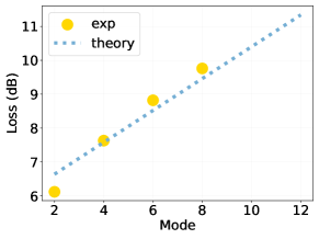
The number of modes of the chip determines the number of spins and bosonic levels that can be simulated from the spin-boson model. To simulate the model on a larger scale, we must consider the impact of increasing on-chip loss as the number of mode increases. Generally, the optical loss primarily depends on the transmission loss caused by the length of the waveguide. Figure A1 shows the experimental measurements of loss for different mode sizes (non-loop identity matrix measurements) and the approximate fitting curve. The results indicate that while optical loss is proportional to the mode number, even for the state-of-the-art in PIC size [41, 42], the loss is experimentally acceptable. These low loss values are largely due to the low-loss SiN waveguides and improvements in fabrication.
| Parameter | Values | |||||||||||||||||||
|---|---|---|---|---|---|---|---|---|---|---|---|---|---|---|---|---|---|---|---|---|
| 0.2 | 0.2 | 0.2 | 0.2 | 0.4 | 0.4 | 0.4 | 0.4 | 0.8 | 0.8 | 0.8 | 0.8 | 1.0 | 1.0 | 1.0 | 1.0 | 1.2 | 1.2 | 1.2 | 1.2 | |
| 0.2 | 0.4 | 0.8 | 1.2 | 0.2 | 1.0 | 0.8 | 1.2 | 0.4 | 1.0 | 0.8 | 1.2 | 0.2 | 0.4 | 1.0 | 1.2 | 0.8 | 0.2 | 0.8 | 1.2 | |
| 0.2 | 1.2 | 1.0 | 0.8 | 0.4 | 1.2 | 1.0 | 0.8 | 0.2 | 1.2 | 1.0 | 0.8 | 0.8 | 1.2 | 1.0 | 0.4 | 0.4 | 1.2 | 1.0 | 0.8 | |
Appendix F Error evaluation and mitigation
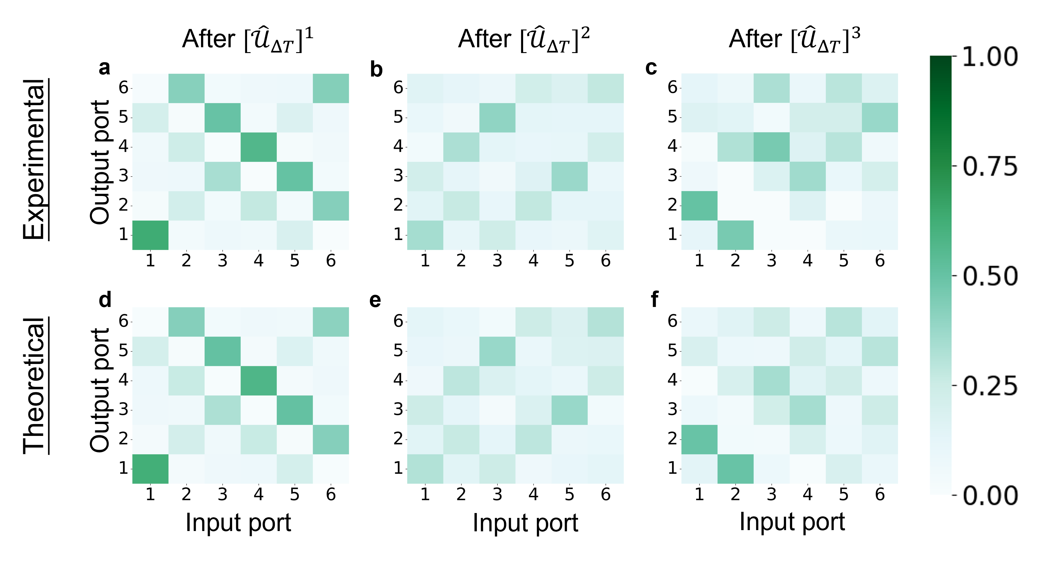
On top of the photon losses, we also need to evaluate the fidelity of reproducing the quantum evolution. To quantify the errors, we consider that the first photon is sent through channel and we record when and in which channel it is measured. Then, for each of the different time steps , we count the frequency of being recorded in each output channel which results in experimental matrices (where indicates the channel in which the photon was measured), which we compare with the theoretically exact results . A very good resemblance is shown in Fig. A2 where panels a-c depict the experimental results and panels d-f the theoretical ones.
To be more quantitative, from these matrices we can then evaluate the error as
| (13) |
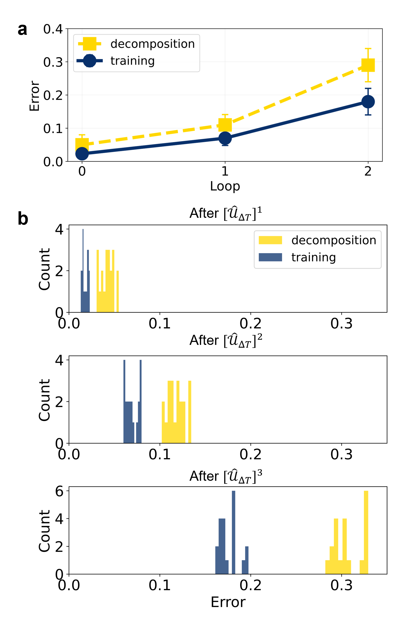
The analysis of errors is depicted in Fig. A3 evaluated across the 20 different preparations of the Hamiltonian parameters in Table 1.
Figure. A3a compares the error distribution of the different evolutions for our trained-based approach (blue) and the Clements et al.’s decomposition (yellow) (see App. B,C for more details). Our training-based approach shows a marked improvement over the decomposition method, demonstrating the effectiveness of this approach. Although the method involves a one-time computational cost for parameter training, once trained, it provides substantial improvements in accuracy. Therefore, when the unitary parameters remain fixed while only the input state varies, the training method offers an advantageous solution for achieving higher computational accuracy. Figure. A3b presents a more detailed insight into the distribution of the error for zero, one, and two loops for these two methods.