Look Back for More: Harnessing Historical Sequential Updates for Personalized Federated Adapter Tuning
Abstract
Personalized federated learning (PFL) studies effective model personalization to address the data heterogeneity issue among clients in traditional federated learning (FL). Existing PFL approaches mainly generate personalized models by relying solely on the clients’ latest updated models while ignoring their previous updates, which may result in suboptimal personalized model learning. To bridge this gap, we propose a novel framework termed pFedSeq, designed for personalizing adapters to fine-tune a foundation model in FL. In pFedSeq, the server maintains and trains a sequential learner, which processes a sequence of past adapter updates from clients and generates calibrations for personalized adapters. To effectively capture the cross-client and cross-step relations hidden in previous updates and generate high-performing personalized adapters, pFedSeq adopts the powerful selective state space model (SSM) as the architecture of sequential learner. Through extensive experiments on four public benchmark datasets, we demonstrate the superiority of pFedSeq over state-of-the-art PFL methods.
Introduction
In recent years, federated learning (FL) (McMahan et al. 2017) has attracted growing research interest for enabling privacy-preserving collaborative model training. However, due to data heterogeneity among clients (i.e. data from different clients are non-IID or unbalanced), it is difficult to develop a one-fits-all global model that performs well on all clients’ local distributions. To address this, personalized federated learning (PFL) (Smith et al. 2017) has emerged. Unlike traditional FL, which develops a single best model for the collective goal, PFL allows each client to have a unique personalized model tailored specifically to the local objective (Li et al. 2021a; Fallah, Mokhtari, and Ozdaglar 2020). Through the collaborative learning scheme, PFL further enables the personalized models to benefit from knowledge sharing across clients, striking a balance between individualization and generalization for enhanced local performance (Kulkarni, Kulkarni, and Pant 2020; Kairouz et al. 2021).

Recently, as large foundation models (FMs) demonstrate impressive capabilities across various tasks, there has seen a rise in research synergizing FL and FMs (Zhuang, Chen, and Lyu 2023). One of the most popular ways of empowering FL with FMs is through parameter-efficient adapter tuning (e.g., LoRA (Hu et al. 2021)), also known as federated adapter tuning (Li et al. 2024; Woisetschläger et al. 2024). This new FL paradigm allows clients to leverage a powerful, pre-trained FM while only fine-tuning and sharing the lightweight adapters with the server, enabling enhanced performance with minimal on-client computation and communication costs. It also opens up opportunities to tailor PFL methods for fine-tuning FM with adapters. For example, leveraging FL for collaborative fine-tuning while personalizing the adapters to better align the representations of pre-trained FM with the local needs of clients (Yi et al. 2023; Xie et al. 2024; Yang et al. 2024).
However, a common limitation of existing PFL and efforts tailored for FM adapter tuning is that they rely solely on the updates received in the most recent round to develop personalized models, while the potentially valuable information contained in previous updates is either underutilized or completely discarded. This can easily lead to noisy and suboptimal solutions, jeopardizing performance when applied to federated adapter tuning personalization. If we view the development of a personalized adapter for a client as an optimization process, focusing only on the latest updates is akin to performing simple gradient descents. By incorporating information from previous updates—much like using momentum in optimization—the learning process accounts for a broader range of past trajectories and uncovers the consistent trends, leading to more robust and reliable personalized solutions at convergence. Hence, in this work, we are motivated to design a framework that accounts for past learning trajectories to develop enhanced personalized adapters. To illustrate, Figure 1 shows the adapter update trajectories of two clients over three rounds of local tuning and communication. As depicted in Figure 1a, existing PFL methods typically rely only on the interactions among the latest updates to produce personalized adapters, which can lead to less robust and undeterministic solutions by only referencing the current states. In contrast, our approach aims to model the interactions among clients at each past update step, as well as the dependencies across various steps, as shown in Figure 1b, which provides a broader perspective for identifying the consistent update patterns, enabling more robust learning and development of more superior personalized adapters.
Specifically, we propose a novel PFL framework termed pFedSeq for improving personalized federated adapter tuning by exploiting knowledge from clients’ past sequential updates. This is achieved through two main processes at the server during each communication round: (1) standard model aggregation using a traditional FL algorithm to obtain a global adapter (e.g., FedAvg (McMahan et al. 2017)), and (2) leveraging a Sequential Learner to process the sequence of clients’ adapter updates collected at the server and output personalized calibrations to adjust the global adapter for clients’ individual needs. To enable flexible modeling of the cross-client and cross-step relations in the sequence, we employ a learnable hypernetwork for the sequential learner, which is jointly trained at the server by optimizing the personalized adapters toward clients’ local objectives. By using the received adapter updates as a proxy for gradients on local losses, the training of sequential learner can be efficiently performed at server without accessing clients’ local data.
Selecting a suitable architecture for the sequential learner is a non-trivial task. To facilitate effective capture of cross-client and cross-step relations, we propose to employ the selective state space model (SSM) (Gu and Dao 2023) as our sequential learner. Selective SSM is a recurrence-based model introduced recently for efficient sequence modeling. It enjoys both effective performance with time-dependent selectivity and efficient computations with linear scaling. To capitalize on its design features, we form the step-wise inputs by concatenating clients’ updates from the same round and processing them in a recurrence mode. With that, the cross-client interactions at different steps can be captured in the time-dependent module parameters, and the sequential processing allows the cross-step dependencies to be captured in the consolidated hidden states.
To summarize, our contributions are as follows:
-
•
We propose a novel PFL framework, pFedSeq, for personalizing federated adapter tuning for clients. By leveraging knowledge from the previous updates, pFedSeq generates enhanced personalized adapters which better tailor large FMs’ representations to clients’ local needs.
-
•
We collaboratively train a sequential learner at the server to capture useful cross-client and cross-step relations in the sequential updates, achieving effective personalized adapter generation by adopting Selective SSM as the learner architecture.
-
•
We evaluate our pFedSeq rigorously on four large-scale benchmark datasets (i.e., CIFAR-100, Tiny-ImageNet, DomainNet, and Omniglot), and show that our pFedSeq outperforms ten state-of-the-art PFL methods by up to 5.39%.
Related Work
Traditional FL algorithms (McMahan et al. 2017; Li et al. 2020; Karimireddy et al. 2020) following the one-model-fits-all paradigm often suffer from degraded performance on clients’ local data in the face of severe data heterogeneity. Recently, personalized FL (PFL) has attracted much attention, which develops customized models to accommodate the diverse needs of clients (Mansour et al. 2020). Generally, efforts in PFL fall under four categories:
(1) Meta-learning-based methods.
By drawing an analogy between FL and meta-learning (Jiang et al. 2019), this approach jointly develops a global model from which the personalized models can be effectively fine-tuned with just a few local steps. Per-FedAvg (Fallah, Mokhtari, and Ozdaglar 2020) adopts the spirit of MAML (Finn, Abbeel, and Levine 2017) and jointly learns a global initialization by optimizing for one-step gradient updates. pFedMe (T Dinh, Tran, and Nguyen 2020) further allows multiple updates in the inner loop and optimizes a Moreau envelope objective.
(2) Personalized-aggregation-based methods.
This line of methods produces personalized models by learning client-specific aggregation weights to combine models from other clients. FedFomo (Huang et al. 2021) and FedAMP (Zhang et al. 2021) leverage a rule-based approach to compute weights based on the pair-wise distance between clients’ models. APPLE (Luo and Wu 2022) and FedALA (Zhang et al. 2023) adopt a learning-based approach to optimize the personalized weights directly on clients’ local objectives. FedDPA (Yang et al. 2024) was introduced recently, focusing on addressing test-time distribution shifts by combining global and personalized adapters through dynamic weighting for federated adapter tuning.
(3) Personalized-network-based methods.
This approach develops a personalized model independently for each client while drawing on the general knowledge through various forms of global sharing. FedRep (Collins et al. 2021) and FedBN (Li et al. 2021b) locally update parts of the network that are sensitive to data distributions (e.g., the classification head or the batch-norm layers), while sharing the rest to leverage the common representations. Ditto (Li et al. 2021a) trains full personalized models locally, using a proximal term to regularize distance from the global model. PerAda (Xie et al. 2024) was recently introduced for federated adapter tuning. It leverages proximal regularization similar to Ditto, while further incorporating knowledge distillation to facilitate information sharing. pFedLoRA (Yi et al. 2023) encourages efficient sharing for model-heterogeneous PFL through lightweight adapters.
(4) Hypernetwork-based methods.
As opposed to solely relying on model aggregation for information sharing, this approach outlines a new way of federation by jointly training a hypernetwork using feedback returned from clients (e.g., the model updates). The hypernetwork is trained to directly generate personalized model parameters based on some inputs. Since it is only trained and maintained at the server, a high-capacity, complex network can be adopted for enhanced diversity of the models generated without concern about the communication costs. pFedHN (Shamsian et al. 2021) is a pioneering work that leverages this approach to generate personalized models for clients based on the learnable client descriptor vectors. L2C (Li et al. 2022) and pFedLA (Ma et al. 2022) utilize hypernetwork to learn personalized aggregation weights. pFedPG (Yang, Wang, and Wang 2023) focuses on federated prompt learning and trains a hypernetwork for personalized prompt generation. PeFLL (Scott, Zakerinia, and Lampert 2024) and FedL2P (Lee et al. 2023) condition on clients’ local statistics and train a hypernetwork to output personalized models or update strategies.
Our work, by collaboratively training a sequential learner, falls under the hypernetwork-based methods. Different from the existing works, we propose to generate personalized adapters by leveraging clients’ previous updates. In other related fields concerning multi-task/distribution learning similar to FL, past gradient updates are commonly used to enhance task representations (Zenke, Poole, and Ganguli 2017; Flennerhag et al. 2018; Peng and Pan 2023) or to derive relations among different parties (Yu et al. 2020; Mansilla et al. 2021). In the realm of FL, (Ji et al. 2019) utilizes previous clients’ updates to produce global model via an RNN-based aggregator. However, the potential of leveraging previous updates for PFL still remains unexplored. Our work fills this gap by developing a method to extract useful cross-client and cross-step relations from past updates, producing personalized adapters that better suit clients’ local specifics.
Method

Preliminaries
Problem Setup.
In a typical FL setup involving clients and a central server, each client has its own private data . Traditional FL (e.g., FedAvg (McMahan et al. 2017)) seeks to learn a global model that performs well across all clients: , where is an arbitrary loss function. However, this one-model-fits-all scheme may fail when data heterogeneity is severe among clients. PFL addresses this by relaxing the single-model constraint and learning personalized models , each tailored specifically to a client, while also benefiting from the federation by drawing knowledge from global model :
Personalized Federated Adapter Tuning.
Adopting adapter tuning in PFL provides a computation- and communication-efficient solution for clients to harness the power of large FMs. Let denote a fixed, pre-trained foundation model backbone (e.g., ViT (Dosovitskiy et al. 2020)), which remains locally at clients. A chosen adapter (e.g., LoRA), denoted by parameterized by , as well as the classification head parameterized by , are tuned at the client to adapt the fixed backbone to local distributions. Since only the adapter and the head are updated and shared with the server, without loss of generality, we define the global and personalized models as and . The individual loss of client is computed by:
pFedSeq Framework
In this section, we present our pFedSeq framework, designed for personalizing federated adapter tuning. Following (Collins et al. 2021; Yang, Wang, and Wang 2023), we update the classification head locally without sharing with the server to better preserve the client-specific knowledge, and apply pFedSeq to generate the personalized adapters.
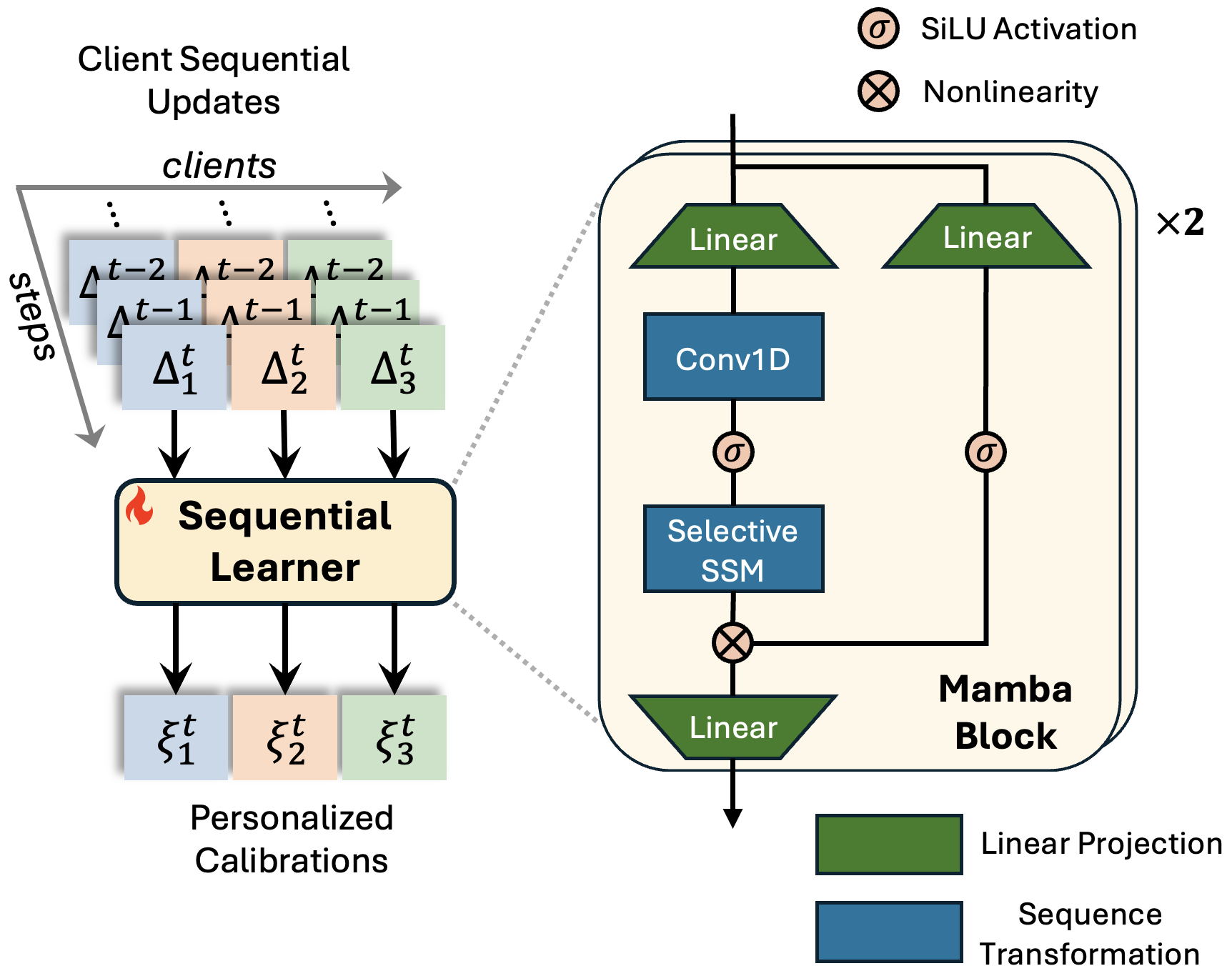
An overview of pFedSeq is shown in Figure 2. At each communication round, pFedSeq performs local adapter tuning at the clients and sends the adapter updates to the server. The server then conducts personalized adapter generation with the sequential learner by processing the sequence of past updates collected from clients. Meanwhile, the server also performs sequential learner optimization using the new updates received from the clients as feedback for training. We now introduce each process in detail.
Local Adapter Tuning at Client.
Suppose we are at the -th local training round of client . Upon receiving the personalized adapter generated by the server in the previous round, we update and jointly on local data for several local epochs to obtain and . Note that is not generated by the server and is restored from the previous local update at client . Also, to be differentiated from the personalized adapter generated by the server, we use to denote the adapter updated locally. We then compute the adapter update and send it to the server.
Personalized Adapter Generation at Server.
To generate personalized adapters, two processes are carried out at the server: (1) aggregating clients’ updated adapters to produce a global adapter, and (2) using the sequential learner to process clients’ past updates and output personalized calibrations for tailoring the global adapter to each client.
Specifically, after the -th communication round, server receives adapter updates from clients. To compute the globally aggregated adapter, we need to obtain the clients’ updated adapters . To avoid doubling the communication costs, we can compute directly using the adapter updates received from the clients and the personalized adapters generated at the server in the previous round, i.e., . By using the classic FedAvg (McMahan et al. 2017) for aggregation, we obtain the global adapter at the -th round:
| (1) |
Simultaneously, we utilize a sequential learner, which is a hypernetwork, to generate personalized calibrations from the sequential updates. Specifically, at the -th round, we construct the input to sequential learner by first stacking across clients for each collected at the server, forming , where is the dimensionality of the adapter’s parameters. We then concatenate across steps, forming the sequence input matrix . The sequential learner, denoted by parameterized by , outputs the personalized calibrations for the clients by taking in the sequence input :
| (2) |
Note that by treating as the batch dimension, we employ one to capture the cross-client and cross-step relations for all parameters of an adapter. Hence, the size of is independent of the adapter size and only depends on the number of clients and the sequence length . For better expressivity, we assign one to learn the parameters of the adapter attached to each layer of the backbone (e.g., ViT-B/16 contains 12 layers (Dosovitskiy et al. 2020)).
Finally, we obtain the personalized adapters for the -th round by adding to the global adapter :
| (3) |
The personalized adapters are sent to the clients for the next round of local training.

Sequential Learner Optimization at Server.
Since the objective of the sequential learner is to generate effective personalized calibrations that perform well on clients’ local data, we optimize the parameters of by:
| (4) |
where . Using chain rule, the gradient update for from each client is given by (note that ). Following (Shamsian et al. 2021; Scott, Zakerinia, and Lampert 2024), we approximate using the adapter update received from client . This is equivalent to replacing a single gradient step on with multiple gradient update steps, which has been shown to achieve better and more stable convergence (Shamsian et al. 2021).
Specifically, at the -th round, we receive adapter updates from clients. Recall that these are the updates from the previous round’s personalized adapters , i.e., is the proxy for gradient evaluated at , indicating the optimization direction at . Hence, we use as the signal to adjust , which constitutes generated by inputting (i.e., sequence until ) to . Formally, we compute the update for at the -th round by:
| (5) | ||||
Remarks.
To avoid infinitely growing sequence length as the number of update rounds increases, we cap the sequence input at a maximum length , i.e., (2) becomes:
| (6) |
Also, to ensure that generates reliable personalized adapters for the next round of local update for stable convergence, we set a warm-up period to sufficiently train before putting it into use. That is, for the first rounds, the server only updates without using it to generate the personalized calibrations, and only the global adapter is sent to clients during the warm-up period. Algorithm 1 summarizes the workflow.
Sequential Learner using Selective SSM
In this section, we introduce an instantiation of the sequential learner using Selective SSM as the learner architecture. Selective SSM is recently introduced for efficient sequence modeling (Gu and Dao 2023). In terms of modeling cross-client and cross-step relations, the selection mechanism of Selective SSM allows cross-client interactions at different steps to be captured in the input-dependent parameters. At the same time, the recursive processing effectively abstracts the cross-step dependencies in the internal hidden states.
Given a sequence input of length , Selective SSM generates output at each step by taking in the previous step hidden state and the current step input , where is an expanded latent dimension. The step-wise modular operation is formulated as follows:
| (7) |
where are discretized parameters, and is a projection matrix, all obtained by conditioning on the current step input (a concatenation of clients’ updates), i.e., (detailed formulations in (Gu and Dao 2023)). Note that we input a sequence into Selective SSM, and optimize or perform inference only on the final-step output . Figure 3b illustrates a step module of Selective SSM.
Following (Gu and Dao 2023), we incorporate a 1D convolution and a residual connection before and after the Selective SSM, forming a Mamba block. A detailed description of our architecture is included in Appendix A.
Experiments
Experimental Setup
Datasets and Heterogeneity Scenarios.
We evaluate our pFedSeq on four benchmark datasets covering three different data heterogeneity scenarios. For label-skew scenario, we use CIFAR-100 (Krizhevsky et al. 2009) which consists of 60,000 images from 100 classes, and Tiny-ImageNet (Chrabaszcz, Loshchilov, and Hutter 2017) which consists of 110,000 images from 200 classes. For both datasets, we simulate label-skew heterogeneity by distributing data in each class over 10 clients with a Dirichlet distribution , following (Yang, Wang, and Wang 2023; Zhang et al. 2023). For feature-skew scenario, we consider DomainNet, which involves 600,000 images from 345 classes across 6 domains (i.e., Clipart, Infograph, Painting, Quickdraw, Real, and Sketch). Following (Li et al. 2021b), we use the top ten most frequent classes for experiments, simulating feature skew across clients by treating each domain as a client (i.e., ). Furthermore, we consider a real-world heterogeneous scenario where data are collected from actual clients. We adopt Omniglot, which contains images of 1,623 characters from 50 alphabets, handwritten by 20 different individuals. We treat each individual as a client (i.e., ) and predict the alphabet to which a character belongs.
Baselines.
We compare the performance of pFedSeq against 12 baselines, including 2 traditional methods and 10 state-of-the-art PFL methods. For traditional baselines, we consider Local and classic FedAvg, where the former performs local adapter tuning only without sharing information with other clients, while the latter aggregates a global adapter and a global head to share with all clients. For PFL baselines, we include meta-learning-based methods Per-FedAvg (Fallah, Mokhtari, and Ozdaglar 2020) and pFedMe (T Dinh, Tran, and Nguyen 2020); personalized-aggregation-based methods APPLE (Luo and Wu 2022) and FedALA (Zhang et al. 2023); personalized-network-based methods FedRep (Collins et al. 2021), Ditto (Li et al. 2021a), and PerAda (Xie et al. 2024); and hypernetwork-based methods pFedHN (Shamsian et al. 2021), pFedLA (Ma et al. 2022), and PeFLL (Scott, Zakerinia, and Lampert 2024). All methods are evaluated on clients’ local test sets, and the final result is computed by averaging over all clients.
Implementation Details.
For fair comparisons, we adapt all compared methods to the same federated adapter tuning setup, where we adopt ViT-B/16 (Dosovitskiy et al. 2020) pre-trained on ImageNet21k (Deng et al. 2009) as the fixed backbone and fine-tune LoRA adapter (Hu et al. 2021). We implement all methods by tuning and sharing only the LoRA and the classification head using the respective PFL algorithms. For all datasets, the number of communication rounds is set to 80. At each round, the clients perform adapter tuning for 1 local epoch using SGD optimizer with a batch size of 32. The local learning rate is set to 0.05 for Omniglot and 0.005 for other datasets. For our pFedSeq, we adopt a 2-layer Mamba as our sequential learner and set the expanded state dimension to 16. We train our sequential learner using Adam optimizer with learning rate 0.001, similarly for other hypernetwork-based methods. For all datasets, we set the number of warm-up rounds to 10 and tune the maximum sequence length in {5, 10, 15, 20, 25, 30}. All experiments are conducted on NVIDIA A100 GPUs with 40GB memory. We repeat each experiment with 3 seeds and report the mean and standard deviation. More implementation details can be found in Appendix B.
Baseline Comparison
| Method | Label-Skew | Feature-Skew | Real-World | |
| CIFAR-100 | Tiny-ImageNet | DomainNet | Omniglot | |
| Local | 92.940.02 | 92.520.11 | 78.670.15 | 38.360.24 |
| FedAvg | 87.360.12 | 87.980.19 | 78.190.19 | 37.870.84 |
| Meta-Learning-Based | ||||
| Per-FedAvg | 93.680.08 | 93.280.03 | 80.620.67 | 40.730.40 |
| pFedMe | 93.350.10 | 93.620.04 | 81.710.28 | 41.900.44 |
| Personalized-Aggregation-Based | ||||
| APPLE | 93.380.08 | 93.230.01 | 80.340.81 | 40.350.72 |
| FedALA | 93.730.02 | 93.300.02 | 81.170.76 | 39.860.46 |
| Personalized-Network-Based | ||||
| FedRep | 94.060.11 | 93.010.18 | 81.310.48 | 38.040.10 |
| Ditto | 93.870.05 | 93.460.02 | 80.740.90 | 41.180.46 |
| PerAda | 93.910.07 | 93.430.02 | 80.930.85 | 41.720.53 |
| Hypernetwork-Based | ||||
| pFedHN | 94.460.37 | 93.510.18 | 81.980.40 | 42.480.19 |
| pFedLA | 93.420.21 | 93.370.11 | 80.260.20 | 41.270.55 |
| PeFLL | 94.410.05 | 93.700.26 | 82.420.17 | 42.980.18 |
| pFedSeq | 95.300.09 | 94.300.08 | 84.630.24 | 45.250.16 |
Table 1 compares the performance of pFedSeq against baselines applied to the same federated adapter tuning setup. On all the four datasets, our pFedSeq achieves the highest performance, with significant margins of {0.84%, 0.6%, 2.21%, 2.27%} over the second-best performer (i.e., pFedHN or PeFLL). Notably, we observe greater gains for DomainNet and Omniglot characterized by distinct domain discrepancies across clients. This demonstrates the efficacy of our method in personalizing adapters to better adjust the backbone representations for different styles or feature distributions. Throughout Table 1, we observe that all PFL methods outperform Local and FedAvg, indicating their effectiveness in balancing global and local knowledge. As compared to meta-learning and personalized-network methods, which drive the personalized adapters too closely to the global model (through common initialization or regularization), our pFedSeq directly produces diverse personalized calibrations that better adjust the global adapter to clients’ local specifics, leading to better results. Unlike aggregation-based methods, which linearly combine client-specific adapters, pFedSeq leverages the non-linearity of a hypernetwork to model the complex client relations and achieves better knowledge transfer. A closer look at Table 1 reveals that hypernetwork-based methods, such as pFedHN, PeFLL, and our pFedSeq, outshine other types of methods, demonstrating the advantages of using hypernetworks to directly produce small-sized adapters. Our pFedSeq, by using the sequential learner to capture the cross-client and cross-step relations, further outperforms the existing hypernetwork-based methods. More discussions on baseline comparisons are included in Appendix C.

In Figure 4, we show the learning curves of pFedSeq and compared baselines over 80 communication rounds for CIFAR-100 and Tiny-ImageNet (the plots for DomainNet and Omniglot are included in Appendix C). For clearer visualization, we only present the curves of representative baselines under each PFL category. From the plots, we can see that our pFedSeq (blue line) begins to outperform all the baselines at around the 25-th round. Though our pFedSeq shows similar performance to FedRep (green line) during the warm-up phase (i.e., the first 10 rounds), where only the global adapter is sent out for clients’ local evaluation, we observe rapid improvement once pFedSeq begins to use the personalized adapters generated by the stably trained sequential learner, quickly surpassing all baselines in 15 rounds. The accelerated learning demonstrates the advantages of leveraging previous update steps for deriving more robust and superior personalized adapters, which enables a positive feedback loop between enhanced local updates and better generated personalized adapters, facilitating faster learning and improved performance at convergence.
Analysis of pFedSeq
In this section, we first conduct experiments to verify the effectiveness of the various design components of pFedSeq. Then, we provide detailed analysis of the impact of the maximum sequence length on the performance of pFedSeq.
Effectiveness of Key Components.
We examine how the three key components of pFedSeq (i.e., global aggregation, cross-step modeling, cross-client modeling) contribute to its overall performance by introducing three variants: variant A removes global aggregation from pFedSeq and uses the sequential learner to generate personalized adapters directly instead of personalized calibrations; variant B eliminates cross-step modeling by using only the latest updates from all clients to generate personalized calibrations, equivalent to setting ; variant C eliminates cross-client modeling by generating the personalized calibration for a client using only that client’s sequential updates.
As shown in Table 2, we see that removing global aggregation results in the largest performance drops: 0.89% for CIFAR-100 and 1.96% for DomainNet, signifying the importance of directly leveraging the knowledge sharing through the global adapter. Also, we note that even without global aggregation, variant A performs comparably to the strongest baselines (e.g., pFedHN and PeFLL), which shows the effectiveness of the cross-step and cross-client modeling for directly generating the personalized adapters. Next, we see that removing either cross-step or cross-client modeling leads to significant performance drops on both datasets: 0.64% and 0.9% for CIFAR-100, and 1.53% and 0.78% for DomainNet, indicating the importance of taking into account both and exploiting their coupled effects in our design. In addition, we observe that both variants B and C surpass the strongest baselines on the two datasets, which shows that even when considered individually, either cross-step or cross-client modeling is effective for generating enhanced personalized adapters.
| Variant | global aggregation | cross-step modeling | cross-client modeling | CIFAR-100 | DomainNet |
| A | ✗ | ✓ | ✓ | 94.410.11 | 82.670.26 |
| B | ✓ | ✗ | ✓ | 94.660.08 | 83.100.36 |
| C | ✓ | ✓ | ✗ | 94.400.12 | 83.850.23 |
| pFedSeq | ✓ | ✓ | ✓ | 95.300.09 | 84.630.24 |
| Variant | Learner Architecture | CIFAR-100 | DomainNet |
| D | MLP | 94.320.17 | 81.250.56 |
| E | LSTM | 94.690.23 | 82.770.36 |
| pFedSeq | Selective SSM | 95.300.09 | 84.630.24 |
Effectiveness of Learner Architecture.
To verify our choice of using Selective SSM as the sequential learner, we further introduce two variants using different architectures. First, variant D employs an MLP-based network similar to (Shamsian et al. 2021) for the sequential learner, where the sequence of inputs are concatenated along a single dimension (i.e., ) and passed into the MLP network. Note that this architecture can only process fixed-length sequences. As shown in Table 3, using an MLP learner leads to performance drops of 0.98% for CIFAR-100 and 3.38% for DomainNet. The decline is mainly attributed to the less effective structure of MLP for modeling sequence inputs, leading to instability of training (as can be observed in Figure 9 in Appendix C). As for the second architecture, variant E utilizes the classical LSTM (Hochreiter and Schmidhuber 1997) for the learner. Similar to Selective SSM, LSTM is capable of modeling variable-length sequences. However, it reuses the same cell for all the steps without selectivity, making it less capable of discerning valuable context information from different steps. Table 3 shows that using an LSTM learner leads to performance declines of 0.61% on CIFAR-100 and 1.86% on DomainNet. The less satisfactory performance of variants D and E on two datasets demonstrates the superiority of using Selective SSM to model the cross-client and cross-step dependencies for more effective personalization.

Impact of Maximum Sequence Length .
We investigate the impact of by varying it in a more fine-grained range {1, 3, 5, 7, 9, 11, 13, 15} on Omniglot dataset. The results are plotted in Figure 5, where the dotted line indicates the performance of the strongest baseline PeFLL as a reference. From the plot, we can clearly observe an increasing trend in the performance of pFedSeq as the maximum sequence length increases. As compared to modeling only on the latest updates (i.e., ), modeling on a longer sequence of previous updates (i.e., ) results in 1.17% increase in the performance of pFedSeq. This further confirms the effectiveness of our approach in modeling previous sequential updates. Moreover, the performance appears to plateau at a certain level, with further increases in yielding minimal improvements. This may be because earlier updates that are too distant from the present offer less relevant information, making them less useful for generating personalized adapters for the next update round. To achieve the best trade-off between computational cost and performance, we tune to find the elbow point where the performance starts to plateau. Overall, our pFedSeq outperforms PeFLL even with , signifying the effectiveness of our choice of architecture in generating personalized calibrations, and our global aggregation process for explicitly leveraging the global knowledge. A plot of the learning curves for different values of is included in Appendix C.
Conclusion
In this paper, we propose a novel pFedSeq framework for personalizing federated adapter tuning by exploiting knowledge from clients’ previous updates. Our pFedSeq introduces a sequential learner jointly trained across all clients at the server to capture the cross-client and cross-step relations from the sequential updates, and output effective personalized adapters. For the learner architecture, we employ the powerful Selective SSM to leverage its sequence modeling capabilities. Extensive experiments on four benchmark datasets demonstrate the superiority of pFedSeq over ten state-of-the-art PFL methods and verify the effectiveness of its various components through rigorous studies.
Acknowledgments
This research is supported by the RIE2025 Industry Alignment Fund – Industry Collaboration Project (IAF-ICP) (Award No: I2301E0020), administered by A*STAR.
References
- Chrabaszcz, Loshchilov, and Hutter (2017) Chrabaszcz, P.; Loshchilov, I.; and Hutter, F. 2017. A downsampled variant of imagenet as an alternative to the cifar datasets. arXiv preprint arXiv:1707.08819.
- Collins et al. (2021) Collins, L.; Hassani, H.; Mokhtari, A.; and Shakkottai, S. 2021. Exploiting shared representations for personalized federated learning. In International conference on machine learning, 2089–2099. PMLR.
- Deng et al. (2009) Deng, J.; Dong, W.; Socher, R.; Li, L.-J.; Li, K.; and Fei-Fei, L. 2009. Imagenet: A large-scale hierarchical image database. In 2009 IEEE conference on computer vision and pattern recognition, 248–255. Ieee.
- Dosovitskiy et al. (2020) Dosovitskiy, A.; Beyer, L.; Kolesnikov, A.; Weissenborn, D.; Zhai, X.; Unterthiner, T.; Dehghani, M.; Minderer, M.; Heigold, G.; Gelly, S.; et al. 2020. An Image is Worth 16x16 Words: Transformers for Image Recognition at Scale. In International Conference on Learning Representations.
- Fallah, Mokhtari, and Ozdaglar (2020) Fallah, A.; Mokhtari, A.; and Ozdaglar, A. 2020. Personalized federated learning with theoretical guarantees: a model-agnostic meta-learning approach. In Proceedings of the 34th International Conference on Neural Information Processing Systems, 3557–3568.
- Finn, Abbeel, and Levine (2017) Finn, C.; Abbeel, P.; and Levine, S. 2017. Model-agnostic meta-learning for fast adaptation of deep networks. In International conference on machine learning, 1126–1135. PMLR.
- Flennerhag et al. (2018) Flennerhag, S.; Moreno, P. G.; Lawrence, N. D.; and Damianou, A. 2018. Transferring Knowledge across Learning Processes. In International Conference on Learning Representations.
- Gu and Dao (2023) Gu, A.; and Dao, T. 2023. Mamba: Linear-time sequence modeling with selective state spaces. arXiv preprint arXiv:2312.00752.
- Hochreiter and Schmidhuber (1997) Hochreiter, S.; and Schmidhuber, J. 1997. Long short-term memory. Neural computation, 9(8): 1735–1780.
- Hu et al. (2021) Hu, E. J.; Wallis, P.; Allen-Zhu, Z.; Li, Y.; Wang, S.; Wang, L.; Chen, W.; et al. 2021. LoRA: Low-Rank Adaptation of Large Language Models. In International Conference on Learning Representations.
- Huang et al. (2021) Huang, Y.; Chu, L.; Zhou, Z.; Wang, L.; Liu, J.; Pei, J.; and Zhang, Y. 2021. Personalized cross-silo federated learning on non-iid data. In Proceedings of the AAAI conference on artificial intelligence, volume 35, 7865–7873.
- Ji et al. (2019) Ji, J.; Chen, X.; Wang, Q.; Yu, L.; and Li, P. 2019. Learning to learn gradient aggregation by gradient descent. In Proceedings of the 28th International Joint Conference on Artificial Intelligence, 2614–2620.
- Jiang et al. (2019) Jiang, Y.; Konečnỳ, J.; Rush, K.; and Kannan, S. 2019. Improving federated learning personalization via model agnostic meta learning. arXiv preprint arXiv:1909.12488.
- Kairouz et al. (2021) Kairouz, P.; McMahan, H. B.; Avent, B.; Bellet, A.; Bennis, M.; Bhagoji, A. N.; Bonawitz, K.; Charles, Z.; Cormode, G.; Cummings, R.; et al. 2021. Advances and open problems in federated learning. Foundations and trends® in machine learning, 14(1–2): 1–210.
- Karimireddy et al. (2020) Karimireddy, S. P.; Kale, S.; Mohri, M.; Reddi, S.; Stich, S.; and Suresh, A. T. 2020. Scaffold: Stochastic controlled averaging for federated learning. In International conference on machine learning, 5132–5143. PMLR.
- Krizhevsky et al. (2009) Krizhevsky, A.; et al. 2009. Learning multiple layers of features from tiny images.
- Kulkarni, Kulkarni, and Pant (2020) Kulkarni, V.; Kulkarni, M.; and Pant, A. 2020. Survey of personalization techniques for federated learning. In 2020 fourth world conference on smart trends in systems, security and sustainability (WorldS4), 794–797. IEEE.
- Lee et al. (2023) Lee, R.; Kim, M.; Li, D.; Qiu, X.; Hospedales, T.; Huszár, F.; and Lane, N. D. 2023. FedL2P: federated learning to personalize. In Proceedings of the 37th International Conference on Neural Information Processing Systems, 14818–14836.
- Li et al. (2024) Li, S.; Ye, F.; Fang, M.; Zhao, J.; Chan, Y.-H.; Ngai, E. C.-H.; and Voigt, T. 2024. Synergizing Foundation Models and Federated Learning: A Survey. arXiv preprint arXiv:2406.12844.
- Li et al. (2022) Li, S.; Zhou, T.; Tian, X.; and Tao, D. 2022. Learning to collaborate in decentralized learning of personalized models. In Proceedings of the IEEE/CVF Conference on Computer Vision and Pattern Recognition, 9766–9775.
- Li et al. (2021a) Li, T.; Hu, S.; Beirami, A.; and Smith, V. 2021a. Ditto: Fair and robust federated learning through personalization. In International conference on machine learning, 6357–6368. PMLR.
- Li et al. (2020) Li, T.; Sahu, A. K.; Zaheer, M.; Sanjabi, M.; Talwalkar, A.; and Smith, V. 2020. Federated optimization in heterogeneous networks. Proceedings of Machine learning and systems, 2: 429–450.
- Li et al. (2021b) Li, X.; JIANG, M.; Zhang, X.; Kamp, M.; and Dou, Q. 2021b. FedBN: Federated Learning on Non-IID Features via Local Batch Normalization. In International Conference on Learning Representations.
- Luo and Wu (2022) Luo, J.; and Wu, S. 2022. Adapt to adaptation: Learning personalization for cross-silo federated learning. In IJCAI: proceedings of the conference, volume 2022, 2166. NIH Public Access.
- Ma et al. (2022) Ma, X.; Zhang, J.; Guo, S.; and Xu, W. 2022. Layer-wised model aggregation for personalized federated learning. In Proceedings of the IEEE/CVF conference on computer vision and pattern recognition, 10092–10101.
- Mansilla et al. (2021) Mansilla, L.; Echeveste, R.; Milone, D. H.; and Ferrante, E. 2021. Domain generalization via gradient surgery. In Proceedings of the IEEE/CVF international conference on computer vision, 6630–6638.
- Mansour et al. (2020) Mansour, Y.; Mohri, M.; Ro, J.; and Suresh, A. T. 2020. Three approaches for personalization with applications to federated learning. arXiv preprint arXiv:2002.10619.
- McMahan et al. (2017) McMahan, B.; Moore, E.; Ramage, D.; Hampson, S.; and y Arcas, B. A. 2017. Communication-efficient learning of deep networks from decentralized data. In Artificial intelligence and statistics, 1273–1282. PMLR.
- Peng and Pan (2023) Peng, D.; and Pan, S. J. 2023. Clustered task-aware meta-learning by learning from learning paths. IEEE transactions on pattern analysis and machine intelligence, 45(8): 9426–9438.
- Scott, Zakerinia, and Lampert (2024) Scott, J.; Zakerinia, H.; and Lampert, C. H. 2024. PeFLL: Personalized federated learning by learning to learn. In The Twelfth International Conference on Learning Representations.
- Shamsian et al. (2021) Shamsian, A.; Navon, A.; Fetaya, E.; and Chechik, G. 2021. Personalized federated learning using hypernetworks. In International Conference on Machine Learning, 9489–9502. PMLR.
- Smith et al. (2017) Smith, V.; Chiang, C.-K.; Sanjabi, M.; and Talwalkar, A. 2017. Federated multi-task learning. In Proceedings of the 31st International Conference on Neural Information Processing Systems, 4427–4437.
- T Dinh, Tran, and Nguyen (2020) T Dinh, C.; Tran, N.; and Nguyen, J. 2020. Personalized federated learning with moreau envelopes. Advances in neural information processing systems, 33: 21394–21405.
- Woisetschläger et al. (2024) Woisetschläger, H.; Isenko, A.; Wang, S.; Mayer, R.; and Jacobsen, H.-A. 2024. A survey on efficient federated learning methods for foundation model training. arXiv preprint arXiv:2401.04472.
- Xie et al. (2024) Xie, C.; Huang, D.-A.; Chu, W.; Xu, D.; Xiao, C.; Li, B.; and Anandkumar, A. 2024. PerAda: Parameter-Efficient Federated Learning Personalization with Generalization Guarantees. In Proceedings of the IEEE/CVF Conference on Computer Vision and Pattern Recognition, 23838–23848.
- Yang, Wang, and Wang (2023) Yang, F.-E.; Wang, C.-Y.; and Wang, Y.-C. F. 2023. Efficient model personalization in federated learning via client-specific prompt generation. In Proceedings of the IEEE/CVF International Conference on Computer Vision, 19159–19168.
- Yang et al. (2024) Yang, Y.; Long, G.; Shen, T.; Jiang, J.; and Blumenstein, M. 2024. Dual-Personalizing Adapter for Federated Foundation Models. arXiv preprint arXiv:2403.19211.
- Yi et al. (2023) Yi, L.; Yu, H.; Wang, G.; and Liu, X. 2023. Fedlora: Model-heterogeneous personalized federated learning with lora tuning. arXiv preprint arXiv:2310.13283.
- Yu et al. (2020) Yu, T.; Kumar, S.; Gupta, A.; Levine, S.; Hausman, K.; and Finn, C. 2020. Gradient surgery for multi-task learning. In Proceedings of the 34th International Conference on Neural Information Processing Systems, 5824–5836.
- Zenke, Poole, and Ganguli (2017) Zenke, F.; Poole, B.; and Ganguli, S. 2017. Continual learning through synaptic intelligence. In International conference on machine learning, 3987–3995. PMLR.
- Zhang et al. (2023) Zhang, J.; Hua, Y.; Wang, H.; Song, T.; Xue, Z.; Ma, R.; and Guan, H. 2023. Fedala: Adaptive local aggregation for personalized federated learning. In Proceedings of the AAAI Conference on Artificial Intelligence, volume 37, 11237–11244.
- Zhang et al. (2021) Zhang, M.; Sapra, K.; Fidler, S.; Yeung, S.; and Alvarez, J. M. 2021. Personalized Federated Learning with First Order Model Optimization. In International Conference on Learning Representations.
- Zhuang, Chen, and Lyu (2023) Zhuang, W.; Chen, C.; and Lyu, L. 2023. When foundation model meets federated learning: Motivations, challenges, and future directions. arXiv preprint arXiv:2306.15546.
Appendix A A. Model Architecture of Sequential Learner
Full Architecture
In practice, we adopt two layers of Mamba as our sequential learner, as shown in Figure 6. Following the implementation by Gu and Dao (2023), we insert a normalization layer and a residual connection before and after each Mamba block. Within each Mamba block, the input is first linearly projected to a higher dimension and split into two parts, where the first part undergoes 1D depthwise convolution along the step dimension followed by a SiLU activation and Selective SSM, and the second part is for residual connection with the Selective SSM output.
Complexity Analysis
By adopting Mamba with Selective SSM as the core mechanism for sequence processing, we now analyze how its space complexity (i.e., model parameter size, intermediate activations during execution) depends on various input dimensions. Recall that we construct the input to the sequential learner as , where is the adapter’s parameter size, is the number of clients, and is the sequence length. Since the adapter’s parameter size is along the batch dimension, the size of the sequential learner is independent of the adapter’s size. This is in contrast to other hypernetwork-based methods, which aim to learn the mapping in a high-dimensional parameter space, resulting in the hypernetwork’s size increasing with the size of the client’s network. In our case, the size of the learnable Mamba parameters depends only on the number of clients , which scales far less significantly than the adapter’s (or any target network’s) dimension . The internal operations along the step dimension (i.e., 1D convolution and Selective SSM) also result in memory consumption increasing linearly with the sequence length . To avoid extensive memory usage of computing a large along the batch dimension, one can perform equivalent batch updates in practice, e.g., using a batch size of 32 and performing update steps.
Regarding time complexity, although the selection mechanism prevents the parallel convolution of SSM, Selective SSM adopts an efficient parallel scan algorithm to replace the sequential recurrence, which effectively reduces the number of necessary sequential steps from to , i.e., the time complexity is lowered to log-linear.
Appendix B B. Implementation Details
Data Split and Preprocessing
We simulate three data heterogeneity scenarios using four datasets. CIFAR-100 and Tiny-ImageNet are used to simulate the label-skew scenario by distributing data from each class to clients following a Dirichlet distribution with , which is commonly referred to as a practical non-IID setting (Zhang et al. 2021, 2023). Figure 7 shows the data distributions for CIFAR-100 and Tiny-ImageNet among 10 clients used in our experiments. DomainNet dataset is used to simulate the feature-skew scenario by treating each domain as a client, and Omniglot dataset is used to simulate a real-world Internet of Things where each individual is a client.

For CIFAR-100, Tiny-ImageNet, and Omniglot, we follow Zhang et al. (2023) to split the local data for each client into training and test sets with a 25/75 ratio. For DomainNet, we conduct experiments using the top ten most common classes and follow the train-test split from Li et al. (2021b). We hold out 10% of the training data as the validation set.
All input images are resized to with bicubic interpolation to match the input dimensions of ViT-B/16. Each image tensor is normalized with a mean of 0.5 and a standard deviation of 0.5 for all channels.
Hyperparameter Settings
The experimental pipeline for baseline comparisons was developed based on Zhang et al. (2023)’s PFLlib codebase. For all baselines, we tune the hyperparameters by performing grid search from a set of values on held-out validation set.
For Per-FedAvg and pFedMe, due to the additional updates for the inner-loop optimization, the local learning rate is a sensitive hyperparameter. We tune the local learning rate in {0.001, 0.005, 0.01, 0.05} for all four datasets, setting it to 0.01 for DomainNet and Omniglot, and to 0.005 for CIFAR-100 and Tiny-ImageNet.
For APPLE, we set the learning rate for the aggregation weights (also termed the directed relationship vector) to 0.001, after tuning from {0.001, 0.01, 0.1, 1.0}. For FedALA, we apply adaptive local aggregation (ALA) to the adapters attached at all layers of the backbone. The learning rate for ALA is set to 0.1, tuned from {0.001, 0.01, 0.1, 1.0}, and the convergence threshold (i.e., the standard deviation of adjacent losses) is set to 1.0 to avoid long training time of ALA optimization.
For FedRep, we follow the key idea of learning feature representations globally and the classification head locally by performing global aggregation on the adapters attached to all layers of the backbone (i.e., the feature extractor) and learning the classification heads locally for each client. For Ditto and PerAda, we set the coefficient for the proximal term to 0.1, tuning from {0.01, 0.1, 1.0, 10.0}. For PerAda, knowledge distillation (KD) is performed using CIFAR-10 (Krizhevsky et al. 2009) as the auxiliary dataset. The number of KD steps for training the global adapter is set to 100 for a better trade-off between computational cost and performance, and the learning rate for KD is set to 0.005, tuned from {0.001, 0.005, 0.01, 0.05}.
For pFedHN, pFedLA, and PeFLL, the hypernetworks for generating the adapter’s parameters or the layer-wise aggregation weights are adopted from their original implementations. pFedHN employs a 4-layer MLP to compute the clients’ embeddings from a set of learnable clients’ descriptor vectors and a fully connected layer to generate the adapter’s parameters at each backbone layer. The hidden size is set to 100. pFedLA adopts a similar hypernetwork architecture as pFedHN but assigns a unique hypernetwork to generate each client’s embedding and uses the last fully connected layer to compute the layer-wise aggregation weights for combining client-specific adapters. For PeFLL, an embedding network is used to generate the clients’ descriptor vectors based on the raw local data, which adopts a LeNet-style ConvNet with 2 convolutional layers (with filter size and output channel size 32) followed by 3 fully connected layers. The hypernetwork for generating the adapter’s parameters is similar to pFedHN. For all three hypernetwork-based baselines, the learning rate is tuned in {0.0001, 0.0005, 0.001, 0.005, 0.01}, and set to 0.001 for CIFAR-100, Tiny-ImageNet and DomainNet, and 0.0005 for Omniglot. Adam optimizer is used for updating the hypernetworks in all three methods.
For our pFedSeq, we employ a 2-layer Mamba as our sequential learner. The expand factor of the linear projection within each Mamba block is set to 2, and the kernel size of the 1D convolution is set to 4. We set the expanded state dimension to 16, tuned from {4, 8, 16, 32}. The maximum sequence length is set to for CIFAR-100 and Tiny-ImageNet, and for DomainNet and Omniglot, tuned from {5, 10, 15, 20, 25, 30}, taking into account a better trade-off between performance and computational efficiency. We use Adam optimizer for training the sequential learner and tune the learning rate similarly to the other hypernetwork-based methods.
Appendix C C. Additional Results
Computational Efficiency of Baselines
| Method | Label-Skew | Feature-Skew | Real-World | |
| CIFAR-100 | Tiny-ImageNet | DomainNet | Omniglot | |
| Local | 754.7 | 1720.0 | 197.7 | 479.7 |
| FedAvg | 758.8 | 1720.7 | 197.8 | 480.5 |
| Meta-Learning-Based | ||||
| Per-FedAvg | 763.7 | 2163.8 | 242.3 | 607.0 |
| pFedMe | 3796.5 | 7040.8 | 989.8 | 2254.7 |
| Personalized-Aggregation-Based | ||||
| APPLE | 818.4 | 2167.3 | 269.1 | 656.5 |
| FedALA | 1529.2 | 3096.7 | 474.3 | 892.7 |
| Personalized-Network-Based | ||||
| FedRep | 1512.1 | 3441.4 | 395.5 | 960.8 |
| Ditto | 1425.5 | 3436.2 | 452.7 | 1048.2 |
| PerAda | 1735.8 | 3753.8 | 655.3 | 1622.2 |
| Hypernetwork-Based | ||||
| pFedHN | 758.4 | 1721.0 | 198.3 | 476.4 |
| pFedLA | 760.3 | 1722.6 | 204.8 | 482.1 |
| PeFLL | 824.1 | 1805.3 | 270.1 | 531.3 |
| pFedSeq | 761.3 | 1721.7 | 198.3 | 483.6 |
In Table 4, we report the average time taken (in seconds) per communication round for each method on four datasets. The time accounts for local training at client, as well as aggregation and any additional computations at server. Therefore, we use the average time taken per round to reflect and compare the computational efficiency. From the results, we can see that our pFedSeq is among the most efficient PFL methods (comparable to pFedHN and pFedLA). Compared to the Local baseline, our pFedSeq achieves significant performance gains with only a few additional seconds. The extra time taken is mainly due to the update (i.e., backward pass) and inference (i.e., forward pass) on the sequential learner at the server, where both processes are performed once per communication round (i.e., a single-step full-batch update and a single forward pass).
| Method | Data Distribution | Backbone | Communicated Parameter Size | CIFAR-100 Performance |
| Personalized-Aggregation-Based | ||||
| FedFomo (Huang et al. 2021) | 15 clients, pathological non-IID | ConvNet-based | 104k | 40.94 |
| FedAMP (Zhang et al. 2021) | 100 clients, practical non-IID | ResNet18 | 6.4m | 54.27 |
| FedALA (Zhang et al. 2023) | 20 clients, practical non-IID () | ConvNet-based | 104k | 55.92 |
| Personalized-Network-Based | ||||
| FedRep (Collins et al. 2021) | 100 clients, pathological non-IID | ConvNet-based | 60.8k | 56.10 |
| pFedLoRA (Yi et al. 2023) | 10 clients, pathological non-IID | Trainable ConvNet-based + LoRA Tuning | 35k | 75.58 |
| Hypernetwork-Based | ||||
| pFedHN (Shamsian et al. 2021) | 10 clients, pathological non-IID | ConvNet-based | 104k | 68.15 |
| L2C (Li et al. 2022) | 100 clients, pathological non-IID | ConvNet-based | 104k | 59.00 |
| pFedLA (Ma et al. 2022) | 10 clients, pathological non-IID | ConvNet-based | 104k | 47.22 |
| PeFLL (Scott, Zakerinia, and Lampert 2024) | 100 clients, pathological non-IID | ConvNet-based | 128k | 56.00 |
| pFedPG (Yang, Wang, and Wang 2023) | 10 clients, practical non-IID () | Frozen ViT-B/16 + Prompt Tuning | 7.68k | 55.91 |
| pFedSeq (Ours) | 10 clients, practical non-IID () | Frozen ViT-B/16 + LoRA Tuning | 73k | 95.30 |
As compared to other PFL methods, our pFedSeq is significantly more efficient than FedRep, Ditto and PerAda, which require additional training at local clients to separately learn the local and global components or to optimize the proximal term. PerAda performs additional training of the global model at server through distillation on an auxiliary dataset, making it the most costly among the three. Our pFedSeq is also more efficient than the learning-based aggregation methods APPLE and FedALA, which require explicit optimization of the personalized aggregation weights on clients’ local data. pFedMe is the most costly among the compared PFL methods, due to the multi-step inner-loop optimization performed at each local update. Hypernetwork-based methods are arguably the most efficient, as the updates on the hypernetwork can be computed efficiently using feedback returned by clients, and the personalized adapters are generated conveniently by a single forward pass.
As compared to the hypernetwork-based counterparts like pFedHN and pFedLA, our pFedSeq which operates on sequences of inputs is only slightly slower (note that the computation time of pFedSeq reported here is based on ). Thanks to the efficient parallel scan of Selective SSM to replace the sequential recurrence computations, the computational time of pFedSeq is reduced from linear in sequence length to log-linear, allowing it to handle long sequences with only a slight increase in computation time. Also, by directly using the stored model updates as inputs, pFedSeq is more efficient than PeFLL, which requires additional training of clients’ descriptors based on clients’ local data. Overall, our pFedSeq ranks 2nd or 3rd among eleven PFL methods in terms of computational efficiency, while achieving the best performance (with significant margins over the second-best performers pFedHN or PeFLL).
Comparison of PFL Baselines in Original Setup
In our experiments, we adapt all PFL baselines to the same federated adapter tuning setup (i.e., fine-tuning a frozen ViT with LoRA) to ensure fair comparisons. Here, we provide the results of PFL baselines on CIFAR-100 as reported in the literature under the original setups used by the authors. The setups differ in the backbone model used at local clients, and the way the data is distributed among clients. These PFL baselines also have different communication costs depending on the backbone model used and the requirements of the PFL algorithms.
In Table 5, we record the data distribution method, the backbone used, the communicated parameter size, and the performance on CIFAR-100 as reported in their original papers for several PFL baselines. Generally, the local test performance is largely determined by the capability of the backbone model, where our setup of tuning LoRA on a powerful, pre-trained ViT results in much better performance as compared to most of the PFL baselines that utilize ConvNet-based model as the backbone. Unlike the traditional setup of updating the full backbone model, federated adapter tuning, which updates only the lightweight adapter, leads to a much smaller parameter size to be transmitted and reduced computational overhead at clients. Perhaps the most similar setup to ours is the recent work pFedPG, which distributes data among 10 clients using and leverages a pre-trained ViT-B/16. Note that pFedPG fine-tunes the ViT using prompt tuning while ours employs LoRA adapter tuning. By learning only the personalized prompts for each client, pFedPG maintains the smallest communicated parameter size. However, this approach also limits the effectiveness of adapting the ViT to local clients, resulting in significantly poorer performance compared to adapter tuning. Overall, Table 5 showcases the advantages of adopting adapter tuning in PFL, which achieves a better trade-off between communication costs (as well as local computation costs) and local personalization performance.
Additional Figures
This section includes learning curve plots (of baselines or variants) for the various studies discussed in the main paper.

Figure 8 shows the learning curves of pFedSeq and representative PFL baselines on DomainNet and Omniglot. Similar to Figure 4, pFedSeq exhibits comparable performance to FedRep during the warm-up phase (i.e., the first 10 rounds) and quickly surpasses all the baselines within 15 rounds on DomainNet and 5 rounds on Omniglot, demonstrating the effectiveness of the personalized adapters generated by pFedSeq in facilitating faster learning and boosting performance.

Figure 9a presents the learning curves of the three variants introduced in the analysis of key components on CIFAR-100 and DomainNet (see Table 2 in the main paper for a recall of these three variants). From the plots, we observe that for DomainNet, removing global aggregation (red line) significantly degrades performance and leads to unstable learning. On CIFAR-100, the abrupt drop of the red line after the warm-up phase (when switching from the global adapter to personalized adapters directly generated by the sequential learner) also demonstrates the importance of global aggregation in stabilizing the learning process. Removing cross-client modeling (green line) and focusing on clients’ own update trajectories may lead to faster learning in the earlier phase after warm-up. However, this variant is eventually outperformed by pFedSeq, indicating the importance of considering cross-client knowledge transfer to alleviate overfitting to local data and promote better generalization. Lastly, removing cross-step modeling (orange line), equivalent to setting , results in less stable learning and poorer performance at convergence compared to our pFedSeq, which considers a longer sequence of updates for generating personalized adapters (here, we set for CIFAR-100 and for DomainNet). This demonstrates the effectiveness of incorporating past updates for improved learning.
Figure 9b shows the learning curves of two variants using alternative architectures: MLP and LSTM, for the sequential learner (see Table 3 in the main paper for a recall of these two variants). From the plots, we can see that employing an MLP-based network (orange line) seriously degrades the learning stability. This is mainly due to that, by simply concatenating the sequence inputs along a single dimension, the temporal information inherent in the inputs at various steps is lost, leading to less effective modeling of the sequential dependencies. Moreover, treating a sequence of inputs as one long token and processing it with fully connected layers is less efficient, giving rise to more complex modeling and adversely affecting learning stability. Utilizing an LSTM-based network (orange line) for the sequential learner leads to more stable and improved sequence modeling performance compared to the MLP-based network. However, reusing the same cell across all steps limits the model’s capacity to discern valuable information from the context, whereas Selective SSM with its input-dependent selection mechanism effectively addresses this issue, leading to enhanced performance. Moreover, by replacing sequential recurrence with parallel scan, Selective SSM is also more efficient than traditional RNN-based networks like LSTM which suffer from linear time complexity.

In our framework, we allocate a certain warm-up period to allow the sequential learner to be sufficiently trained before applying it to generate personalized adapters for the next round. We investigate the impact of by varying it in {5, 10, 15, 20, 25, 30, 35, 40} and testing the performance on DomainNet. The results are shown in Figure 11. First, we can see that without sufficiently warming up the sequential learner (e.g., ), the performance attained is relatively lower. This is because utilizing an inadequately trained sequential learner to generate personalized adapters may adversely affect the next round of local updates and the subsequent global aggregation, leading to suboptimal convergence. Also, applying a short warm-up period can lead to less stable training, as evidenced by the larger variance. Instead, increasing warm-up period to 10 leads to 1.21% increase in performance and 0.30% drop in standard deviation compared to . Though further increasing the warm-up period slightly improves the final performance (i.e., performance attained at the 80-th communication round), we set the warm-up period to 10 in all our experiments to avoid prolonged warm-up, during which clients can only receive the less capable global adapter for local evaluation and deployment. Also, a long warm-up period is not favorable for convergence efficiency. Overall, our pFedSeq outperforms PeFLL for all the values of tested. A plot of the learning curves for different values of is shown in Figure 12.

