Longitudinal Canonical Correlation Analysis

For each subject $i=1,...,n$ and visits $j=1,\ldots,J_{i}$, we observe the $p$-dimensional vector $\mathbf{X}_{ij}$ at time $t_{ij}$. Similarly, for the visits $k=1,\ldots,K_{i}$, we observe a $q$-dimensional vector $\mathbf{Y}_{ik}$ at time $s_{ik}$. For illustration, we consider the linear trajectories for each variable and later we generalize to the nonlinear trajectories via spline regression. We model each observation using a random intercept and slope model:

where $\mathbf{\mu}_{ij}^{X}$ and $\mathbf{\mu}_{ik}^{Y}$ are fixed effects; $\mathbf{Z}_{i,0}^{X}$ and $\mathbf{Z}_{i,0}^{Y}$ are random intercepts; $\mathbf{Z}_{i,1}^{X}$ and $\mathbf{Z}_{i,1}^{Y}$ are random slopes; ${\boldsymbol{\epsilon}}_{ij}^{X}$ and ${\boldsymbol{\epsilon}}_{ik}^{Y}$ are errors. The random effects are stacked to a $2p$-dimensional vector $\mathbf{Z}_{i}^{X}:=\big{(}{{\mathbf{Z}}_{i,0}^{X}}^{\prime},{{\mathbf{Z}}_{i,1}^{X}}^{\prime}\big{)}^{\prime}\in\mathbb{R}^{2p}$ , and a $2q$-dimensional vector ${\mathbf{Z}}_{i}^{Y}:=\big{(}{{\mathbf{Z}}_{i,0}^{Y}}^{\prime},{{\mathbf{Z}}_{i,1}^{Y}}^{\prime}\big{)}^{\prime}\in\mathbb{R}^{2q}$, and are assumed to be distributed with zero mean and a covariance ${\boldsymbol{\Sigma}}_{c}=\left[\begin{array}[]{rr}{\boldsymbol{\Sigma}}_{c}^{(0,0)}&{\boldsymbol{\Sigma}}_{c}^{(0,1)}\\ {\boldsymbol{\Sigma}}_{c}^{(1,0)}&{\boldsymbol{\Sigma}}_{c}^{(1,1)}\\ \end{array}\right]$, where ${\boldsymbol{\Sigma}}_{c}^{(a,b)}=\mathbb{E}\left({\mathbf{Z}}_{i,a}^{c}{{\mathbf{Z}}_{i,b}^{c}}^{\prime}\right)$, $a,b\in\{0,1\},c\in\{X,Y\}$ and uncorrelated with ${\boldsymbol{\epsilon}}_{ij}^{X}$ and ${\boldsymbol{\epsilon}}_{ik}^{Y}$. The random intercepts, slopes and errors are assume to follow a Gaussian distribution.

Then, the objective function defining the canonical correlation is

When $p$ is greater than $n/2$, we can employ principal component analysis to represent $\mathbf{Z}_{i}^{X}\approx{\boldsymbol{\Phi}}_{X}{\boldsymbol{\xi}}_{i}^{X}$, where ${\boldsymbol{\Phi}}_{X}=\left({{\boldsymbol{\Phi}}_{0}^{X}}^{\prime},{{\boldsymbol{\Phi}}_{1}^{X}}^{\prime}\right)^{\prime}$ is a $2p\times N_{X}$ matrix of the leading $N_{X}$ eigenvectors of ${\boldsymbol{\Sigma}}_{X}=Var(\mathbf{Z}_{i}^{X})$ and ${\boldsymbol{\xi}}_{i}^{X}=(\xi_{i1}^{X},\ldots,\xi_{iN_{X}}^{X})^{\prime}\in\mathbb{R}^{N_{X}}$ are the associated subject $i$-specific eigenscores. Using longitudinal principal component analysis (LPCA) (Greven et al., 2011; Zipunnikov et al., 2014; Lee et al., 2015), each term is expressed as

where $(\xi_{il_{1}}^{X},\xi_{il_{2}}^{X})\sim(0,0;\lambda_{X}^{l_{1}},\lambda_{X}^{l_{2}};0)$, in which “$\cdot\sim(\mu_{1},\mu_{2};\sigma_{1}^{2},\sigma_{2}^{2};\rho)$” represents that a pair of gaussian variables has a distribution with mean $(\mu_{1},\mu_{2})$, variance $(\sigma_{1}^{2},\sigma_{2}^{2})$, and correlation $\rho$. Similarly, $\mathbf{Y}_{ik}$ are expressed as

where $(\xi_{il_{1}}^{Y},\xi_{il_{2}}^{Y})\sim(0,0;\lambda_{Y}^{l_{1}},\lambda_{Y}^{l_{2}};0)$. The eigenvectors of (4) and (5) can be obtained by the least-squares estimation of the covariance matrices. Without loss of generality, we assume $\mathbf{X}_{ij}$ is demeaned to have mean zero. The p × p-covariance of $\mathbf{X}_{ij_{1}}$ and $\mathbf{X}_{ij_{2}}$ is given by

where ${\boldsymbol{\Sigma}}_{X}^{\epsilon}$ is the covariance matrix of $\epsilon_{ij}^{X}$ and $\delta_{j_{1},j_{2}}=1$ if $j_{1}=j_{2}$ and $\delta_{j_{1},j_{2}}=0$ otherwise. Denote $vec(\cdot)$ as the vectorization of a matrix by stacking columns of the matrix on top of one another. Then, we can form a matrix $\mathbf{K}_{X}=\{vec({\boldsymbol{\Sigma}}_{X}^{(0,0)}),vec({\boldsymbol{\Sigma}}_{X}^{(0,1)}),vec({\boldsymbol{\Sigma}}_{X}^{(1,0)}),vec({\boldsymbol{\Sigma}}_{X}^{(1,1)}),$ $vec({\boldsymbol{\Sigma}}_{X}^{\epsilon})\}$ and $\mathbf{f}_{ij_{1}j_{2}}=(1,t_{ij_{2}},t_{ij_{1}},t_{ij_{1}}t_{ij_{2}},\delta_{j_{1},j_{2}})^{\top}$ such that $Evec(\mathbf{X}_{ij_{1}}\mathbf{X}_{ij_{2}}^{\top})=\mathbf{K}_{X}\mathbf{f}_{ij_{1}j_{2}}$. By concatenating all vectors across all subjects and visits, we obtain a moment matrix identity for the $p^{2}\times J$ matrix $\mathbf{X}$: $\mathbf{X}=\mathbf{K}_{X}\mathbf{F}$, where $J=\sum_{i=1}^{N}J_{i}^{2}$. Then covariance parameters $\mathbf{K}_{X}$ can be unbiasedly estimated by using ordinary least squares (OLS): $\widehat{\mathbf{K}}_{X}=\mathbf{XF}^{\top}(\mathbf{FF}^{\top})^{-1}$. Given the estimated covariance matrix, the eigenvectors are computed via eigen decomposition. Given the eigenvectors, the eigenscores are estimated by the best linear unbiased predictors (BLUP) from the equations (4) and (5) as discussed in Greven et al. (2011); Zipunnikov et al. (2014).

Denote the $N\times N_{X}$ matrix ${\boldsymbol{\xi}}^{X}=\{\xi_{il}^{X}\}_{i=1,\ldots,N;l=1,\ldots,N_{X}}$ and $N\times N_{Y}$ matrix ${\boldsymbol{\xi}}^{Y}=\{\xi_{il}^{Y}\}_{i=1,\ldots,N;l=1,\ldots,N_{Y}}$. Then, the objective function defining the canonical correlation is

The objective function in (7) is maximized under the restriction that each $\mathbf{u}_{m}$ is orthogonal to the lower order $\mathbf{u}_{m^{\prime}}$, with $1\leq m<m^{\prime}\leq min(N_{X},N_{Y})$. Same restriction is applied for $\mathbf{v}_{m}$ of the second set of variates. For identification purpose, we require a normalization condition for the canonical variates, $\mathbf{u}_{m}^{\top}{\boldsymbol{\xi}}_{i}^{X},\mathbf{v}_{m}^{\top}{\boldsymbol{\xi}}_{i}^{Y},m=1,.\dots,min(N_{X},N_{Y})$, to have unit variance. The canonical vectors are estimated in the lower-dimensional space, and the $m$-th longitudinal canonical vectors are computed as $\left(\mathbf{\Phi}_{0}^{X}+t_{ij}\mathbf{\Phi}_{1}^{X}\right)\mathbf{u}_{m}$ and $\left(\mathbf{\Phi}_{0}^{Y}+s_{ik}\mathbf{\Phi}_{1}^{Y}\right)\mathbf{v}_{m}$ for $m=1,...,min(N_{X},N_{Y})$.

Depending on the availability of time points, this formation can be naturally extended to higher-order trends or modeled via B-spline basis expansion. Assume that the trajectory of the imaging measure at location $v$ is represented by a spline function with fixed knot sequence $\tau_{1}<\cdots<\tau_{D}$ and fixed degree $d$.

where the $b_{r}$ are a set of basis functions and $Z_{i,r}(v)$ are the associated spline coefficients. The $(D+d+1)V$-dimensional stacked vector of $\mathbf{Z_{i}}=(\mathbf{Z}_{i,1}^{\top},\ldots,\mathbf{Z}_{i,D+d+1}^{\top})^{\top}$ can be approximated by the principal component analysis: $\mathbf{Z_{i}}\approx\sum_{l=1}^{N_{X}}\xi_{il}^{X}\mathbf{\Phi}_{l}^{X}$ with each element expressed as $Z_{i,r}(v)\approx\sum_{l=1}^{N_{X}}\xi_{il}^{X}\Phi_{l}^{X,r}(v)$, for $r=1,\ldots,D+d+1$. Then, (8) is reorganized as

Similarly, $Y$ is modeled as

This method does not require that $X$’s and $Y$’s are observed at the same time. As long as they are observed within a time frame that the research question asks, the proposed method can extract association patterns.

To determine the dimension of the CCA, we employ a traditional likelihood ratio test-based approach in the latent space. Starting with $m=0$, we test the null hypothesis $H_{0}$: $d=m$ versus the alternative hypothesis $H_{1}$: $d>m$. If $H_{0}$ is rejected, $m$ is incremented and a new test is conducted. This proceeds until $H_{0}$ is not rejected or $m$ reaches $M=min(N_{X},N_{Y})$. For a given number of canonical variates, $m$, the Wilk’s test statistics (Wilks, 1935; Bartlett, 1947; Friederichs and Hense, 2003) is given by

Based on Rao’s F-approximation (Rao et al., 1973), $F=df_{2}/df_{1}(1-\Lambda_{m}/(\Lambda_{m}))^{1/\nu}$ follows asymptotically $F_{df_{1},df_{2}}$, where $\nu=\sqrt{(df_{1}^{2}-4)/((N_{X}-m)^{2}+(N_{Y}-m)^{2}-5)}$, $df_{1}=(N_{X}-m)*(N_{Y}-m)$, and $df_{2}=(n-1.5-(N_{X}+N_{Y})/2)\nu-df_{1}/2+1$.

The performance of LCCA depends on the selection of $N_{X}$ and $N_{Y}$. Previous works suggested using 80% threshold of the variance explained by the number of individual components (Greven et al., 2011; Lee et al., 2015) or pre-specified numbers (Zipunnikov et al., 2014). In practice, the performance depends on the signal-to-noise ratio, which is particularly relevant for imaging applications. Our numerical experiments show good performance using a threshold of 80-90% as a rule of thumb. The algorithms are implemented as an R package LCCA and available in github (https://seonjoo.github.io/lcca/).

We apply our LCCA method to the ADNI data to identify longitudinal associations between brain morphometry and amyloid deposition. The data were downloaded from the ADNI database (http://adni.loni.usc.edu). The initial phase (ADNI-1) recruited 800 participants, including approximately 200 healthy controls, 400 patients with late mild cognitive impairment (MCI), and 200 patients clinically diagnosed with probable AD over 50 sites across the United States and Canada and followed up at 6- to 12-month intervals for 2–3 years. ADNI has been followed by ADNI-GO and ADNI-2 for existing participants and enrolled additional individuals, including early MCI. To be classified as MCI in ADNI, a subject needed an inclusive Mini-Mental State Examination score of between 24 and 30, subjective memory complaint, objective evidence of impaired memory calculated by scores of the Wechsler Memory Scale Logical Memory II adjusted for education, a score of 0.5 on the Global Clinical Dementia Rating, absence of significant confounding conditions such as current major depression, normal or near-normal daily activities, and absence of clinical dementia.

All studies were approved by their respective institutional review boards and all subjects or their surrogates provided informed consent compliant with HIPAA regulations. In total, the analysis included PET-MRI scan pairs of 680 subjects on average 2.7 ($\pm$ 0.79) visits over 3.7 ($\pm$1.66) years on average. There are 291 cognitively normal (CN), 365 mild cognitive impairment (MCI), and 24 AD participants at baseline. Detailed characteristics of these individuals are given in Table 1.

For internal consistency, 3.0 MPRAGE T1-weighted MR images were used. Cross-sectional image processing was performed using FreeSurfer Version 6. Region of interest (ROI)-specific cortical thickness and volume measures were extracted from the automated FreeSurfer v6 anatomical parcellation using the Desikan-Killiany Atlas (Desikan et al., 2006) for cortical regions; there were 68 ROIs (34 each on the left and right hemispheres), in which the longitudinal cortical thickness and volume measures were collected. The volume measures from 28 subcortical regions (Fischl et al., 2002) were computed, including Lateral Ventricle, Inferior Lateral Ventricle, Thalamus, Caudate, Putamen, Pallidum, Hippocampus, Amygdala, Accumbens area, Third Ventricle, Fourth Ventricle, and five corpus callosum subregions. In addition, the total intracranial volume was included.

We computed amyloid SUVR levels using the PetSurfer pipeline (Greve et al., 2014, 2016), which is available with Freesurfer version 6. The PetSurferpipeline first registers the PET image with the corresponding MRI scan, then applies Partial Volume Correction, and finally resamples the voxel-wise SUVR values onto the cortical surface. The 81 ROI-level summary was computed based on Desikan Atlas for the cortical and subcortical regions.

There are no existing CCA methods to handle the longitudinal data’s missing and irregular temporal sampling. Thus, we consider the following approach. First, we computed the intercept and slope of each variable for each subject. Then, within each modality, the vectors of intercepts and slopes were stacked, and we performed a canonical correlation analysis. Finally, the number of canonical variates was estimated in the same principles described in Section 2.2. We named this approach the naive approach.

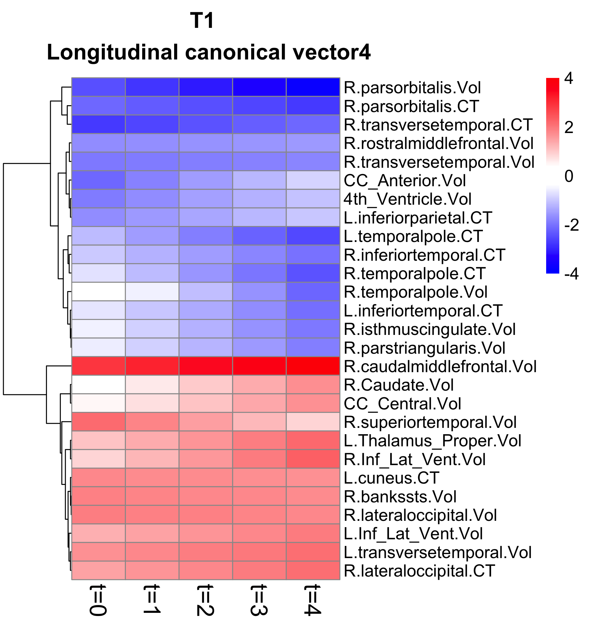
The longitudinal CCA identified 7 canonical variates. The significant canonical correlation coefficients are displayed in Figure 1. The longitudinal canonical vectors were reorganized as a function of time $\left(\mathbf{\Phi}_{0}^{X}+t\mathbf{\Phi}_{1}^{X}\right)\mathbf{u}_{m}$ and $\left(\mathbf{\Phi}_{0}^{Y}+s\mathbf{\Phi}_{1}^{Y}\right)\mathbf{v}_{m}$ for $m=1,...,min(N_{X},N_{Y})$ are displayed in Figures 2 and 3 at time=0,1,2,3,4. For visualization, the vectors are standardized with the total variance of the vectors, and the ROIs with at least one element of the vector over 1.64 are included in the heatmaps. The rows are clustered using hierarchical cluster analysis with complete linkage to visualize which variables behave similarly over time. Figures 2 and 3 include the longitudinal canonical weights of the six longitudinal canonical variates that are associated with either baseline diagnosis status or AD transition. We also performed naive approach and compared its performance.

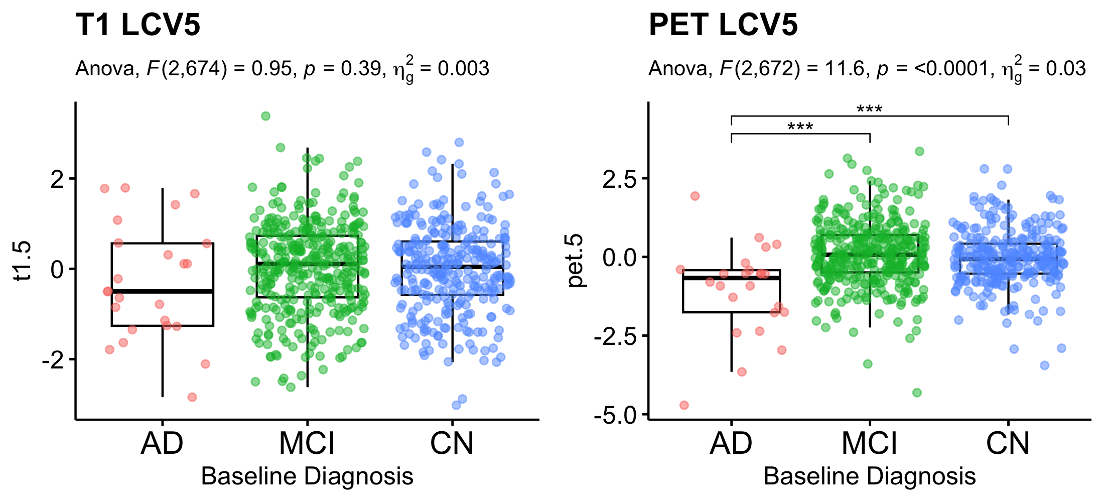
Further, we investigated the longitudinal canonical variates (CV). First, we compared CVs by each subject’s baseline clinical status. For group comparison, linear regression was conducted with age, sex and years of education as covariates, followed by multiple comparison correction controlling for false discovery rate (Benjamini and Hochberg, 1995). Table 2 reports the F-statistics, unadjusted p-values and multiple comparison corrected p-values. For all analyses, we excluded extreme outliers beyond 3 IQR from the first and third quartiles. For post-hoc pair-wise group comparison, least squared mean differences were computed. Figure 6 shows jittered boxplots and pair-wise comparison results with unadjusted p-values for the CVs with significant group difference after multiple comparison correction.

The CV 2, 4, and 7 of T1 and CVs 2 and 5 of PET showed group differences after multiple comparison correction. The CV2 indicates that AD patients at baseline showed atrophy in bilateral hippocampus and amygdala. The amyloid deposition showed a decreased pattern in bilateral Pallidum, and increasing amyloid deposition in the cortical areas (right lingual, right pericalcarine, right fusiform, and inferior temporal cortices). The CV4 of T1 showed the enlarged volume in right caudal middle frontal gyus and longitudinal atrophy in right pars orbitalis in AD and MCI comparing to CN, while PET did not showed any differences. The CV5 of T1 did not show differences across baseline clinical status. The AD patients showed brain atrophy in the left Accumbens area volume, and right paracentral thickness, smaller volume in the left temporal transverse volume and right caudal middle frontal volume, while thicker thickness in the left isthmus cingulate and right lateral orbitofrontal gyrus. The CV5 of av45 showed a longitudinal increase in the left hippocampus and right Pallidum and left paracentral area in AD participants, while MCI and CN participants did not show that pattern on average. CV7 showed enlarged volumes in right lingual gyrus, but atrophy in left caudal ACC and pars orbitals, while no significant difference in amyloid deposition. The naive method identified CV 3 and 5 with significant T1 differences and CVs 9 and 12 for PET. Unlike LCCA, naive method did not identify CVs showed group differences between diagnosis status in both T1 and PET. For AD transition, only CV3 T1 and CV9 PET showed significant group difference.

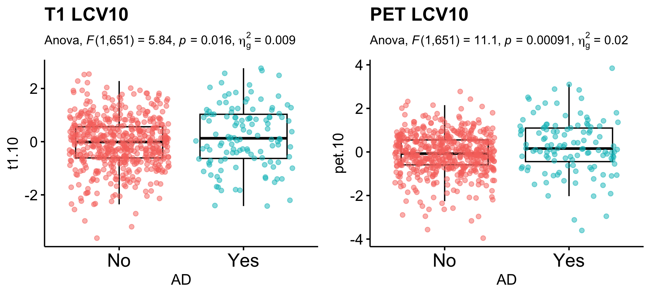
Secondly, among the non-demented participants at baseline, we compared CVs between the participants who translated to AD within 5 years and those who remained non-demented. Among 656 non-demented participants, 120 participants (18.3%) converted to AD in 5 years. Table 2 reports the F-statistics, unadjusted p-values and multiple comparison corrected p-values. For post-hoc pair-wise group comparison, least squared mean differences were computed. Figure 8 shows jittered boxplots and pair-wise comparison results with unadjusted p-values for the CVs with significant group difference after multiple comparison correction. The CVs 1, 2 and 4 for T1 and CVs 1, 2, 4 and 6 of PET showed a significant difference between those who converted to AD and those who did not.

Data were generated from the model 4 setting $N_{X}$ and $N_{Y}$ to 3. The LPC loadings were generated as depicted in Figure 10; we set $p=144$ and $q=81$. The LPC scores ${\xi}_{ik}^{X}$ and $\xi_{ik}^{Y}$ were generated from the $N(0,\lambda_{k})$, $\lambda_{1}=8,\lambda_{2}=4,\lambda_{3}=2$, where $Cor({\xi}_{i2}^{X},{\xi}_{i2}^{Y})=r$. We note that we correlated the second pairs of the LPCs to evaluate LCCA’s performance when the correlated signals explain more minor variances. For each subject, the number of visits were generated from Poisson(1) followed by adding 3 such that each subject has on average 4 time points. The time intervals between visits were generated from $U[1,2]$. Figure 11 shows examples of the time variables $t_{ij}$ and $s_{ik}$ from the first 10 subjects from a simulation setting. The time points between $X$ and $Y$ variables are not aligned, and the numbers of visits differ. We conducted simulations for $r=0.1,0.3,0.5$, at $n=100,200,400$, and different threshold for LPC dimension selection (80% or 90%). For each scenario, 100 independent datasets were generated.

Overall, LCCA outperforms the naive approach in the three criteria. Figure 12 shows that both LCCA and the naive approach tend to overestimate canonical correlation when the sample size is small and the true canonical correlation is smaller, while LCCA performs better than the naive approach. The results show that the approximation-based CV dimension estimation performs better as the sample size increases, and the underlying true canonical correlation is larger. LCCA identifies the number of canonical variates more accurately than the naive approach. Similar patterns were found in the cosine similarity measures. The cosine similarity between estimated LCV loadings performs better as the sample size increases, and the underlying true canonical correlation is larger.

Data were generated similarly to the first simulation, except the first five LPC loadings were taken from ADNI data from Section 3 (Figure 13). The LPC scores ${\xi}_{ik}^{X}$ and $\xi_{ik}^{Y}$ were generated from the $N(0,\lambda_{k})$, $\lambda_{1}=45.4,\lambda_{2}=17.2,\lambda_{3}=7.0,\lambda_{4}=4,1,\lambda_{5}=3.8$, where $Cor({\xi}_{i2}^{X},{\xi}_{i2}^{Y})=r$. For each subject, the number of visits were generated from Poisson(1) followed by adding 3 such that each subject has on average 4 time points. The time intervals between visits were generated from $U[1,2]$. We conducted simulations for $r=0.1,0.3,0.5$, at $n=100,200,400$, and different threshold for LPC dimension selection (80% or 90%). For each scenario, 100 independent datasets were generated. We found very similar results as Simulation 1 (Figure 14, assuring our data analysis results in Section 3 have less bias in estimating canonical weights and correlations. The both methods tend to underestimate canonical correlation when the threshold (=0.8) is smaller, while this issue does not persist when the threshold is more lenient.

We also examined whether the LCCA can recover subgroups. We employed the same simulation settings from Simulation 2, except longitudinal canonical variates (LCVs). Instead of generating the LCVs from a multivariate normal distribution, we imposed two subgroups. One group was generated from $MVN(0,\lambda\mathbf{I}_{2})$ and the other group was generated from $N(\mu\mathbf{1}_{2},\mathbf{I}_{2})$ as shown in Figure 15. We varied the proportion of subsamples from 0.1 to 0.5 and evaluated whether the LCCA can identify subgroups.

To evaluate whether LCCA recovers the true LCVs with subgroups, the correlations between the true and estimated LCVs were calculated. Figure 16 shows that the LCCA identified LCVs, LC vectors, and the number of LCVs well, even with smaller sample sizes and a highly unbalanced subgroups (subsample proportion=0.1).

References

- Adhikari et al. (2019) Adhikari, B. M., Hong, L. E., Sampath, H., Chiappelli, J., Jahanshad, N., Thompson, P. M., Rowland, L. M., Calhoun, V. D., Du, X., Chen, S. and Kochunov, P. (2019) Functional network connectivity impairments and core cognitive deficits in schizophrenia. Human Brain Mapping.
- Avants et al. (2010) Avants, B. B., Cook, P. A., Ungar, L., Gee, J. C. and Grossman, M. (2010) Dementia induces correlated reductions in white matter integrity and cortical thickness: A multivariate neuroimaging study with sparse canonical correlation analysis. NeuroImage, 50, 1004–1016.
- Bao et al. (2019) Bao, Z., Hu, J., Pan, G. and Zhou, W. (2019) Canonical correlation coefficients of high-dimensional Gaussian vectors: Finite rank case. The Annals of Statistics, 47, 612–640.
- Bartlett (1947) Bartlett, M. (1947) The general canonical correlation distribution. The Annals of Mathematical Statistics, 1–17.
- Benjamini and Hochberg (1995) Benjamini, Y. and Hochberg, Y. (1995) Controlling the false discovery rate: a practical and powerful approach to multiple testing. Journal of the Royal statistical society: series B (Methodological), 57, 289–300.
- Deleus and Van Hulle (2011) Deleus, F. and Van Hulle, M. M. (2011) Functional connectivity analysis of fMRI data based on regularized multiset canonical correlation analysis. Journal of Neuroscience Methods, 197, 143–157.
- Desikan et al. (2006) Desikan, R. S., Ségonne, F., Fischl, B., Quinn, B. T., Dickerson, B. C., Blacker, D., Buckner, R. L., Dale, A. M., Maguire, R. P., Hyman, B. T. et al. (2006) An automated labeling system for subdividing the human cerebral cortex on mri scans into gyral based regions of interest. Neuroimage, 31, 968–980.
- Du et al. (2019) Du, L., Liu, K., Zhu, L., Yao, X., Risacher, S. L., Guo, L., Saykin, A. J. and Shen, L. (2019) Identifying progressive imaging genetic patterns via multi-task sparse canonical correlation analysis: A longitudinal study of the ADNI cohort. Bioinformatics, 35, i474–i483.
- Fang et al. (2016) Fang, J., Lin, D., Schulz, S. C., Xu, Z., Calhoun, V. D. and Wang, Y.-P. (2016) Joint sparse canonical correlation analysis for detecting differential imaging genetics modules. Bioinformatics (Oxford, England), 32, 3480–3488.
- Fischl et al. (2002) Fischl, B., Salat, D. H., Busa, E., Albert, M., Dieterich, M., Haselgrove, C., Van Der Kouwe, A., Killiany, R., Kennedy, D., Klaveness, S. and others (2002) Whole brain segmentation: Automated labeling of neuroanatomical structures in the human brain. Neuron, 33, 341–355.
- Friederichs and Hense (2003) Friederichs, P. and Hense, A. (2003) Statistical inference in canonical correlation analyses exemplified by the influence of north atlantic sst on european climate. Journal of Climate, 16, 522–534.
- Gossmann et al. (2018) Gossmann, A., Zille, P., Calhoun, V. and Wang, Y.-P. (2018) FDR-Corrected Sparse Canonical Correlation Analysis With Applications to Imaging Genomics. IEEE transactions on medical imaging, 37, 1761–1774.
- Greve et al. (2016) Greve, D. N., Salat, D. H., Bowen, S. L., Izquierdo-Garcia, D., Schultz, A. P., Catana, C., Becker, J. A., Svarer, C., Knudsen, G. M., Sperling, R. A. and Johnson, K. A. (2016) Different partial volume correction methods lead to different conclusions: An 18F-FDG-PET study of aging. NeuroImage, 132, 334–343.
- Greve et al. (2014) Greve, D. N., Svarer, C., Fisher, P. M., Feng, L., Hansen, A. E., Baare, W., Rosen, B., Fischl, B. and Knudsen, G. M. (2014) Cortical surface-based analysis reduces bias and variance in kinetic modeling of brain PET data. NeuroImage, 92, 225–236.
- Greven et al. (2011) Greven, S., Crainiceanu, C., Caffo, B. and Reich, D. (2011) Longitudinal functional principal component analysis. In Recent Advances in Functional Data Analysis and Related Topics, 149–154. Springer.
- Grosenick et al. (2019) Grosenick, L., Shi, T. C., Gunning, F. M., Dubin, M. J., Downar, J. and Liston, C. (2019) Functional and Optogenetic Approaches to Discovering Stable Subtype-Specific Circuit Mechanisms in Depression. Biological Psychiatry. Cognitive Neuroscience and Neuroimaging, 4, 554–566.
- Hao et al. (2017) Hao, X., Li, C., Yan, J., Yao, X., Risacher, S. L., Saykin, A. J., Shen, L., Zhang, D. and Alzheimer’s Disease Neuroimaging Initiative (2017) Identification of associations between genotypes and longitudinal phenotypes via temporally-constrained group sparse canonical correlation analysis. Bioinformatics (Oxford, England), 33, i341–i349.
- Kang et al. (2016) Kang, J., Bowman, F. D., Mayberg, H. and Liu, H. (2016) A depression network of functionally connected regions discovered via multi-attribute canonical correlation graphs. NeuroImage, 141, 431–441.
- Kim et al. (2019) Kim, M., Won, J. H., Youn, J. and Park, H. (2019) Joint-connectivity-based sparse canonical correlation analysis of imaging genetics for detecting biomarkers of Parkinson’s disease. IEEE transactions on medical imaging.
- Lee et al. (2015) Lee, S., Zipunnikov, V., Reich, D. S. and Pham, D. L. (2015) Statistical image analysis of longitudinal RAVENS images. Frontiers in neuroscience, 9, 368.
- Lin et al. (2014) Lin, D., Calhoun, V. D. and Wang, Y.-P. (2014) Correspondence between fMRI and SNP data by group sparse canonical correlation analysis. Medical Image Analysis, 18, 891–902.
- Mihalik et al. (2019) Mihalik, A., Ferreira, F. S., Rosa, M. J., Moutoussis, M., Ziegler, G., Monteiro, J. M., Portugal, L., Adams, R. A., Romero-Garcia, R., V\a’ertes, P. E., Kitzbichler, M. G., V\a’aša, F., Vaghi, M. M., Bullmore, E. T., Fonagy, P., Goodyer, I. M., Jones, P. B., Dolan, R. and Mourão-Miranda, J. (2019) Brain-behaviour modes of covariation in healthy and clinically depressed young people. Scientific Reports, 9.
- Mueller et al. (2005) Mueller, S. G., Weiner, M. W., Thal, L. J., Petersen, R. C., Jack, C., Jagust, W., Trojanowski, J. Q., Toga, A. W. and Beckett, L. (2005) The Alzheimer’s Disease Neuroimaging Initiative. Neuroimaging Clinics of North America, 15, 869–877.
- Rao et al. (1973) Rao, C. R., Rao, C. R., Statistiker, M., Rao, C. R. and Rao, C. R. (1973) Linear statistical inference and its applications, vol. 2. Wiley New York.
- Song et al. (2016) Song, Y., Schreier, P. J., Ramírez, D. and Hasija, T. (2016) Canonical correlation analysis of high-dimensional data with very small sample support. Signal Processing, 128, 449–458.
- Weiner et al. (2012) Weiner, M. W., Veitch, D. P., Aisen, P. S., Beckett, L. A., Cairns, N. J., Green, R. C., Harvey, D., Jack, C. R., Jagust, W., Liu, E., Morris, J. C., Petersen, R. C., Saykin, A. J., Schmidt, M. E., Shaw, L., Siuciak, J. A., Soares, H., Toga, A. W., Trojanowski, J. Q. and Alzheimer’s Disease Neuroimaging Initiative (2012) The Alzheimer’s Disease Neuroimaging Initiative: A review of papers published since its inception. Alzheimer’s & Dementia, 8, S1–S68.
- Wilks (1935) Wilks, S. (1935) On the independence of k sets of normally distributed statistical variables. Econometrica, Journal of the Econometric Society, 309–326.
- Wilms and Croux (2016) Wilms, I. and Croux, C. (2016) Robust sparse canonical correlation analysis. BMC Systems Biology, 10, 72.
- Witten et al. (2009) Witten, D. M., Tibshirani, R. and Hastie, T. (2009) A penalized matrix decomposition, with applications to sparse principal components and canonical correlation analysis. Biostatistics, 10, 515–534.
- Zhang et al. (2014) Zhang, Y., Zhou, G., Jin, J., Wang, X. and Cichocki, A. (2014) Frequency recognition in SSVEP-based BCI using multiset canonical correlation analysis. International Journal of Neural Systems, 24, 1450013.
- Zipunnikov et al. (2014) Zipunnikov, V., Greven, S., Shou, H., Caffo, B., Reich, D. S. and Crainiceanu, C. (2014) Longitudinal High-Dimensional Principal Components Analysis with Application to Diffusion Tensor Imaging of Multiple Sclerosis. The annals of applied statistics, 8, 2175.