\DeclareDocumentCommand\dpdv∂∂

Long-Term Fairness with Unknown Dynamics

Tongxin Yin¹¹1These authors contributed equally to this work.
Computer Science and Engineering
University of Michigan
Ann Arbor, MI 48109
[email protected] &Reilly Raab¹¹1These authors contributed equally to this work.
Computer Science and Engineering
University of California, Santa Cruz
Santa Cruz, CA 95064
[email protected]
\ANDMingyan Liu
Computer Science and Engineering
University of Michigan
Ann Arbor, MI 48109
[email protected] &Yang Liu
Computer Science and Engineering
University of California, Santa Cruz
Santa Cruz, CA 95064
[email protected]

Abstract

While machine learning can myopically reinforce social inequalities, it may also be used to dynamically seek equitable outcomes. In this paper, we formalize long-term fairness in the context of online reinforcement learning. This formulation can accommodate dynamical control objectives, such as driving equity inherent in the state of a population, that cannot be incorporated into static formulations of fairness. We demonstrate that this framing allows an algorithm to adapt to unknown dynamics by sacrificing short-term incentives to drive a classifier-population system towards more desirable equilibria. For the proposed setting, we develop an algorithm that adapts recent work in online learning. We prove that this algorithm achieves simultaneous probabilistic bounds on cumulative loss and cumulative violations of fairness (as statistical regularities between demographic groups). We compare our proposed algorithm to the repeated retraining of myopic classifiers, as a baseline, and to a deep reinforcement learning algorithm that lacks safety guarantees. Our experiments model human populations according to evolutionary game theory and integrate real-world datasets.

1 Introduction

As machine learning (ML) algorithms are deployed for tasks with real-world social consequences (e.g., school admissions, loan approval, medical interventions, etc.), the possibility exists for runaway social inequalities (Crawford and Calo, 2016; Chaney et al., 2018; Fuster et al., 2018; Ensign et al., 2018). While “fairness” has become a salient ethical concern in contemporary research, the closed-loop dynamics of real-world systems comprising ML policies and populations that mutually adapt to each other (Fig. 5 in the supplementary material) remain poorly understood.

In this paper, our primary contribution is to consider the problem of long-term fairness, or algorithmic fairness in the context of a dynamically responsive population, as a reinforcement learning (RL) problem subject to constraint. In our formulation, the central learning task is to develop a policy that minimizes cumulative loss (e.g., financial risk, negative educational outcomes, misdiagnoses, etc.) incurred by an ML agent interacting with a human population up to a finite time horizon, subject to constraints on cumulative “violations of fairness”, which we refer to in a single time step as disparity and cumulatively as distortion.

Our central hypothesis is that an RL formulation of long-term fairness may allow an agent to learn to sacrifice short-term utility in order to drive the system towards more desirable equilibria. The core practical difficulties posed by our general problem formulation, however, are the potentially unknown dynamics of the system under control, which must be determined by the RL agent online (i.e., during actual deployment), and the general non-convexity of the losses or constraints considered. Additionally, we address continuous state and action spaces, in general, which preclude familiar methods with performance guarantees in discrete settings.

Our secondary contributions are 1) to show that long-term fairness can be solved within asymptotic, probabalistic bounds under certain dynamical assumptions and 2) to demonstrate that the problem of long-term fairness can also be addressed more flexibly. For theoretical guarantees, we develop L-UCBFair, an online RL method, and prove sublinear bounds on regret (suboptimiality of cumulative loss) and distortion (suboptimality of cumulative disparity) with high probability (Section 3.1). To demonstrate practical solutions without limiting assumptions, we apply R-TD3, an adaptation of a well-known deep reinforcement learning method (viz., TD3) to a Lagrangian relaxation of the central problem with time-dependent regularization. We compare L-UCBFair and R-TD3 to a baseline, myopic policy in interaction with simulated populations initialized with synthetic or real-world data and updated according to evolutionary game theory (Section 4).

This paper considers fairness in terms of statistical regularities across (ideally) socioculturally meaningful groups. Acknowledging that internal conflict exists between different statistical measures of fairness, we show that an RL approach to long-term fairness can mitigate trade-offs between fairness defined on the statistics of immediate policy decision outcomes (Chen et al., 2022), (e.g., acceptance rate disparities (Dwork et al., 2012; Zemel et al., 2013; Feldman et al., 2015)) and underlying distributional parameters (e.g., qualification rate (Raab and Liu, 2021; Zhang et al., 2020)).

1.1 Related Work

Our effort to formalize long-term fairness as a reinforcement learning problem bridges recent work on “fairness in machine learning”, which has developed in response to the proliferation of data-driven methods in society, and “safe reinforcement learning”, which seeks theoretical safety guarantees in the control of dynamical systems.

Dynamics of Fairness in Machine Learning We distinguish long-term fairness from the dynamics of fair allocation problems Joseph et al. (2016); Jabbari et al. (2017); Tang et al. (2021); Liu et al. (2017) and emphasize side-effects of algorithmic decisions affecting future decision problems. By formalizing long-term fairness in terms of cumulative losses and disparities, we iterate on a developing research trend that accounts for the dynamical response of a human population to deployed algorithmic prediction: both as a singular reaction Liu et al. (2018); Hu et al. (2019); Perdomo et al. (2020) or as a sequence of mutual updates to the population and the algorithm Coate and Loury (1993); D’Amour et al. (2020); Zhang et al. (2020); Heidari et al. (2019); Wen et al. (2019); Liu et al. (2020); Hu and Chen (2018); Mouzannar et al. (2019); Williams and Kolter (2019); Raab and Liu (2021). In particular, Perdomo et al. (2020) introduces the concept of “performative prediction”, analyzing the fixed-points of interactions between a population and an algorithmic classifier, but with state treated as a pure function of a classifier’s actions. For more realistic dynamics, Mouzannar et al. (2019) and Raab and Liu (2021) model updates to qualification rates that depend on both previous state and the classifier’s actions, but only treat myopic classifiers that optimize immediate utility (subject to fairness constraints) rather than learning to anticipate dynamical population responses. Wen et al. (2019) adopted reinforcement learning to achieve long-term fairness. However, they explore a setting that is restricted to discrete state and action spaces. In particular, this recommends a tabular explore-then-commit approach to reinforcement learning that does not generalize to continuous spaces and thus cannot be directly used in our setting. In addition, we provide separate and tighter bounds for both utility and disparity.

Safe Reinforcement Learning L-UCBFair furthers recent efforts in safe RL. While “model-based” approaches, in which the algorithm learns an explicit dynamical model of the environment, constitute one thread of prior work Efroni et al. (2020); Singh et al. (2020); Brantley et al. (2020); Zheng and Ratliff (2020); Kalagarla et al. (2021); Liu et al. (2021); Ding et al. (2021), such algorithms are typified by significant time and space complexity. Among “model-free” algorithms, the unknown dynamics of our setting preclude the use of a simulator that can generate arbitrary state-action pairs Xu et al. (2021); Ding et al. (2020); Bai et al. (2022). While Wei et al. (2022) introduce a model-free and simulator-free algorithm, the tabular setting considered is only applicable to discrete state and action spaces. To tackle continuous state space, Ding et al. (2021); Ghosh et al. (2022) consider linear dynamics: Ding et al. (2021) develop a primal-dual algorithm with safe exploration, and Ghosh et al. (2022) use a softmax policy design. Both algorithms are based on the work of Jin et al. (2020), which proposed a least squares value iteration method, using an Upper Confidence Bound (UCB) Auer et al. (2002) to estimate a state-action “ $Q$ ” function. To our knowledge, L-UCBFair is the first model-free, simulator-free RL algorithm that provides theoretical safety guarantees for both discrete and continuous state and action spaces. Moreover, L-UCBFair achieves bounds on regret and distortion as tight as any algorithm thus far with discrete action space Ghosh et al. (2022).

2 Problem Formulation

A binary classification task is an initial motivating example for our formulation of long-term fairness, though the formal problem we propose is more widely applicable. To this initial task, we introduce “fairness” constraints, then population dynamics, and then cumulative loss and “disparity”, before formalizing the problem of optimizing cumulative loss subject to constraints on cumulative disparity.

We provide notation for the binary classification task: a random individual, sampled i.i.d. from a population, has features $X\in\mathbf{R}^{d}$ , a label $Y\in\{-1,1\}$ , and a demographic group $G\in\mathcal{G}$ (where $\mathcal{G}=[n]$ for $n\geq 2$ ). Denote the joint distribution of these variables in the population as $s\coloneqq\Pr(X,Y,G)$ . The task is to predict $Y$ (as $\hat{Y}$ ) from $X$ and $G$ . Specifically, the task is to choose a classifier $a$ , such that $\hat{Y}\sim a(X,G)$ , that minimizes some bounded loss $\mathscr{L}\in[0,1]$ over $s$ . This basic classification task is

\min_{a}\quad\mathscr{L}(s,a)

Typically, $\mathscr{L}$ corresponds to the expectation value of a loss function $L$ (such as zero-one-loss) defined for individuals drawn from $s$ . We consider this example, but, in general, allow arbitrary, (unit-interval) bounded loss functions $\mathscr{L}$ :

\mathscr{L}(s,a)\stackrel{{\scriptstyle{e.g.}}}{{=}}\operatorname*{E}_{\begin{subarray}{c}X,Y,G\sim s\\ \hat{Y}\sim a(X,G)\end{subarray}}\big{[}L(Y,\hat{Y})\big{]}

The standard “fair” classification task (without a dynamically responsive population) is to constrain classifier $a$ such that the disparity $\mathscr{D}\in[0,1]$ induced on distribution $s$ by $a$ is bounded by some value $c\in[0,1]$ :

\displaystyle\min_{a}\quad\mathscr{L}(s,a)\quad\text{subject to }\quad\mathscr{D}(s,a)\leq c

A standard example of disparity is the expected divergence of group acceptance rates $\beta$ . e.g., when $\mathcal{G}=\{g_{1},g_{2}\}$ ,

	$\displaystyle\mathscr{D}(s,a)$	$\displaystyle\stackrel{{\scriptstyle{e.g.}}}{{=}}\big{\|}\beta_{s,a}(g_{1})-\beta_{s,a}(g_{2})\big{\|}^{2}$
	$\displaystyle\text{where }\beta_{s,a}(g)$	$\displaystyle\coloneqq\Pr_{\begin{subarray}{c}X,Y,G\sim s\\ \hat{Y}\sim a(X,G)\end{subarray}}(\hat{Y}{=}1\mid G{=}g)$

In this example, $\mathscr{D}$ measures the violation of “demographic parity”: the condition under which a classifier achieves group-independent positive classification rates $\forall g,\Pr(\hat{Y}{=}1\mid G{=}g)=\Pr(\hat{Y}{=}1)$ Dwork et al. (2012). In this paper, we also consider measures of fairness based on inherent population statistics (e.g., parity of group qualification rates $\Pr(Y{=}1\mid G{=}g)$ ), which must be driven dynamically Raab and Liu (2021); Zhang et al. (2020). Such notions of disparity are well-suited to an RL formulation of long-term fairness.

State, Action, and Policy

Considering the semantics of iterated classification tasks, we identify the distribution $s\in\mathcal{S}$ of individuals in the population as a state and the classifier $a\in\mathcal{A}$ as an action. While state space $\mathcal{S}$ is arbitrary, we assume that action space $\mathcal{A}$ admits a Euclidean metric, under which it is closed (i.e., $\mathcal{A}$ is isomorphic to $[0,1]^{m},m\in\mathbf{Z}_{>0}$ ). At a given time $\tau$ , $a_{\tau}$ is sampled stochastically according to the current policy $\pi_{\tau}$ : $a_{\tau}\sim\pi_{\tau}(s_{\tau}).$ We assume $s_{\tau}$ is fully observable at time $\tau$ . In practice, $s_{\tau}$ must be approximated from finitely many empirical samples, though this caveat introduces well-understood errors that vanish in the limit of infinitely many samples.

Dynamics

In contrast to a “one-shot” fair classification task, we assume that a population may react to classification, inducing the distribution $s$ to change. Importantly, such “distribution shift” is a well-known, real-world phenomenon that can increase realized loss and disparity when deployed classification policies are fixed Chen et al. (2022). For classification policies that free to change in response to a mutating distribution $s$ , subsequent classification tasks depend on the (stochastic) predictions made in previous tasks. In our formulation, we assume the existence of dynamical kernel $\mathbf{P}$ that maps a state $s$ and action $a$ at time $\tau$ to a distribution over possible states at time $\tau+1$ :

s_{\tau+1}\sim\mathbf{P}(s_{\tau},a_{\tau})

(1)

We stipulate that $\mathbf{P}$ may be initially unknown, but it does not explicitly depend on time and may be reasonably approximated “online”. While real-world dynamics may depend on information other than the current distribution $\Pr(X,Y,G)$ (e.g., exogenous parameters, history, or additional variables of state), we identify $s$ with the current distribution for simplicity in our treatment of long-term fairness.

Reward and Utility

Because standard RL literature motivates maximizing reward rather than minimizing loss, let us define the instantaneous reward $r\in[0,1]$ and a separate, instantaneous “utility” $g\in[0,1]$ for an RL agent as

	$\displaystyle r(s_{\tau},a_{\tau})$	$\displaystyle\coloneqq 1-\mathscr{L}(s_{\tau},a_{\tau})$		(2)
	$\displaystyle g(s_{\tau},a_{\tau})$	$\displaystyle\coloneqq 1-\mathscr{D}(s_{\tau},a_{\tau})$		(3)

where $r$ and $g$ do not explicitly depend on time $\tau$ .

Value and Quality Functions

Learnable dynamics inspire us to optimize anticipated cumulative reward, given constraints on anticipated cumulative utility. Let $j$ represent either reward $r$ or utility $g$ . We use the letter $V$ (for “value”) to denote the future expected accumulation of $j$ over steps $[h,...,H]$ (without time-discounting) starting from state $s$ , using policy $\pi$ . Likewise, we denote the “quality” of an action $a$ in state $s$ with the letter $Q$ . For $j\in\{r,g\}$ ,

	$\displaystyle V_{j,h}^{\pi}(s)$	$\displaystyle=\operatorname*{E}\Big{[}\sum_{\tau=h}^{H}j\big{(}s_{\tau},a_{\tau}\big{)}\|s_{h}=s\Big{]}$		(4)
	$\displaystyle Q_{j,h}^{\pi}(s,a)$	$\displaystyle=\operatorname*{E}\left[\sum_{\tau=h}^{H}j\big{(}s_{\tau},a_{\tau})\big{)}\mid s_{h}=s,a_{h}=a\right]$		(5)

By the boundedness of $r,g\in[0,1]$ , $V$ and $Q$ belong to the interval $[0,H-h+1]$ .

“Long-term fairness” via reinforcement learning

The central problem explored in this paper is

\displaystyle\max_{\pi}\quad V_{r,1}^{\pi}(s)\quad\text{subject to }\quad V_{g,1}^{\pi}(s)\geq\tilde{c}

(6)

We emphasize that this construction of long-term fairness considers a finite time horizon of $H$ steps and denote the optimal value of $\pi$ as $\pi^{\star}$ .

Assumption 2.1 (Slater’s Condition).

i.e., “strict primal feasibility”: $\exists$ $\gamma>0$ , $\bar{\pi}$ , such that $V_{g,1}^{\bar{\pi}}\left(s\right)\geq$ $\tilde{c}+\gamma$ .

Slater’s condition is also adopted in Efroni et al. (2020); Ding et al. (2021); Ghosh et al. (2022).

The Online Setting

Given initially unknown dynamics, we formulate long-term fairness for the “online” setting, in which learning is only possible through actual “live” deployment of policy, rather than through simulation. As it is not possible to unconditionally guarantee constraint satisfaction in Eq. 6 over a finite number of episodes, we instead measure two types of regret: one that measures the suboptimality of a policy with respect to cumulative incurred loss, which we will continue to call “regret”, and one that measures the suboptimality of a policy with respect to cumulative induced disparity, which we will call “distortion”. Note that we define regret and distortion in Eq. 7 by marginalizing over the stochasticity of state transitions and the sampling of actions:

	$\displaystyle\operatorname{Regret}(\pi,s_{1})\coloneqq V_{r,1}^{\pi^{*}}\left(s_{1}\right)-V_{r,1}^{\pi}\left(s_{1}\right)$		(7)
	$\displaystyle\operatorname{Distortion}(\pi,s_{1})\coloneqq\max\left[0,\tilde{c}-V_{g,1}^{\pi}\left(s_{1}\right)\right]$		(7)

3 Algorithms and Analysis

We show that it is possible to provide guarantees for long-term fairness in the online setting. Specifically, we develop an algorithm, L-UCBFair, and prove that it provides probabilistic, sublinear bounds for regret and distortion under a linear MDP assumption (3.2) and properly chosen parameters (Section A.1, in the supplementary material). L-UCBFair is the first model-free algorithm to provide such guarantees in the online setting with continuous state and action spaces.

3.1 L-UCBFair

Episodic MDP

L-UCBFair inherits from a family of algorithms that treat an episodic Markov decision process (MDP) Jin et al. (2020). Therefore, we first map the long-term fairness problem to the episodic MDP setting, which we denote as $\text{MDP}(\mathcal{S},\mathcal{A},H,\mathbf{P},\mathscr{L},\mathscr{D})$ . The algorithm runs for $K$ episodes, each consisting of $H$ time steps. At the beginning of each episode, which we index with $k$ , the agent commits to a sequence of policies $\pi^{k}=(\pi_{1}^{k},\pi_{2}^{k},...,\pi_{H}^{k})$ for the next $H$ steps. At each step $h$ within an episode, an action $a_{h}^{k}\in\mathcal{A}$ is sampled according to policy $\pi_{h}^{k}$ , then the state $s_{h+1}^{k}$ is sampled according to the transition kernel $\mathbf{P}(s_{h}^{k},a_{h}^{k})$ . $\mathscr{L}$ and $\mathscr{D}$ are the loss and disparity functions. $s_{1}^{k}$ is sampled arbitrarily with each episode.

Episodic Regret

Because L-UCBFair predetermines its policy for an entire episode, we amend our definition of regret and distortion for the all $HK$ time steps by breaking it into a sum over $K$ episodes of length $H$ .

	$\displaystyle\operatorname{Regret}(K)=\sum_{k=1}^{K}\left(V_{r,1}^{\pi^{*}}\left(s_{1}^{k}\right)-V_{r,1}^{\pi^{k}}\left(s_{1}^{k}\right)\right)$		(8)
	$\displaystyle\operatorname{Distortion}(K)=\max\left[0,\sum_{k=1}^{K}\left(\tilde{c}-V_{g,1}^{\pi^{k}}\left(s_{1}^{k}\right)\right)\right]$		(8)

The Lagrangian

Consider the Lagrangian function $\mathcal{L}$ associated with Eq. 6, with dual variable $\nu\geq 0$ :

\mathcal{L}(\pi,\nu):=V_{r,1}^{\pi}\left(s\right)+\nu\left(V_{g,1}^{\pi}\left(s\right)-\tilde{c}\right)

(9)

L-UCBFair approximately solves the primal problem $\max_{\pi}\min_{\nu}\mathcal{L}(\pi,\nu)$ , which is non-trivial, since the objective function is seldom concave in practical parameterizations of $\pi$ . Let $\nu^{*}$ to denote the optimal value of $\nu$ .

Lemma 3.1 (Boundedness of $\nu^{*}$ ).

For $\bar{\pi}$ and $\gamma>0$ satisfying Slater’s Condition (2.1),

\nu^{*}\leq\frac{V_{r,1}^{\pi*}\left(s_{1}\right)-V_{r,1}^{\pi}\left(s_{1}\right)}{\gamma}\leq\frac{H}{\gamma}\coloneqq\mathscr{V}

Lemma 3.1, defines $H/\gamma=\mathscr{V}$ as an upper bound for the optimal dual variable $\nu^{*}$ . $\mathscr{V}$ is an input to L-UCBFair.

Assumption 3.2 (Linear MDP).

$\text{MDP}(\mathcal{S},\mathcal{A},H,\mathbf{P},\mathscr{L},\mathscr{D})$ is a linear MDP with feature map $\phi:\mathcal{S}\times\mathcal{A}\rightarrow\mathbb{R}^{d}$ : For any $h$ , there exist $d$ signed measures $\mu_{h}=\left\{\mu_{h}^{1},\ldots,\mu_{h}^{d}\right\}$ over $\mathcal{S}$ , such that, for any $\left(s,a,s^{\prime}\right)\in\mathcal{S}\times\mathcal{A}\times\mathcal{S}$ ,

\mathbb{P}_{h}\left(s^{\prime}\mid s,a\right)=\left\langle\phi(s,a),\mu_{h}\left(s^{\prime}\right)\right\rangle,

In addition, there exist vectors $\theta_{r,h},\theta_{g,h}\in\mathbb{R}^{d}$ , such that, for any $(s,a)\in\mathcal{S}\times\mathcal{A}$ ,

r\big{(}s,a\big{)}=\left\langle\phi(s,a),\theta_{r,h}\right\rangle;\quad g(s,a)=\left\langle\phi(s,a),\theta_{g,h}\right\rangle

3.2 addresses the curse of dimensionality when state space $\mathcal{S}$ is the space of distributions over $X,Y,G$ . This assumption is also used in Jin et al. (2020); Ghosh et al. (2022), with a similar assumption made in Ding et al. (2021).

3.1.1 Explicit Construction

L-UCBFair, or “LSVI-UCB for Fairness ” (Algorithm 1) is based on an optimistic modification of a Least-Squares Value Iteration, where optimism is realized by an Upper-Confidence Bound, as in LSVI-UCB Jin et al. (2020). For each $H$ -step episode $k$ , L-UCBFair maintains estimates for $Q^{k}_{r},Q^{k}_{g}$ and a time-indexed policy $\pi^{k}$ . In each episode $k$ , L-UCBFair updates $Q^{k}_{r},Q^{k}_{g}$ , interacts with the environment, and updates the dual variable $\nu_{k}$ (constant in $k$ ).

LSVI-UCB Jin et al. (2020)

The estimation of $Q$ is challenging. Consider the Bellman equation: $\forall(s,a)\in\mathcal{S}\times\mathcal{A},$

Q_{h}^{\star}(s,a)\leftarrow\left[r_{h}+\operatorname*{E}_{s^{\prime}\sim\mathbf{P}_{h}(\cdot\mid s,a)}\max_{a^{\prime}\in\mathcal{A}}Q_{h+1}^{\star}\left(\cdot,a^{\prime}\right)\right](s,a)

It is impossible to iterate over all $s,a$ pairs, since $\mathcal{S}$ and $\mathcal{A}$ are continuous. Instead, LSVI parameterizes $Q_{h}^{\star}(s,a)$ by the linear form $\mathrm{w}_{h}^{\top}\phi(s,a)$ , which is supported by Jin et al. (2020). As an additional complication, $\mathbf{P}$ is unknown is estimated by LSVI from empirical samples. Combining these techniques, the Bellman equation can be replaced by a least squares problem.

\displaystyle\mathbf{w}_{h}\leftarrow\underset{\mathbf{w}\in\mathbb{R}^{d}}{\operatorname{argmin}}\sum_{\tau=1}^{k-1}

\displaystyle\bigg{[}r_{h}\left(s_{h}^{\tau},a_{h}^{\tau}\right)+\max_{a\in\mathcal{A}}Q_{h+1}\left(s_{h+1}^{\tau},a\right)-\mathbf{w}^{\top}\phi\left(s_{h}^{\tau},a_{h}^{\tau}\right)\bigg{]}^{2}+\varsigma\|\mathbf{w}\|^{2}

In addition, a “bonus term” $\beta\left(\phi^{\top}\Lambda_{h}^{-1}\phi\right)^{1/2}$ is added to the estimate of Q to encourage exploration.

Adaptive Search Policy Compared to the works of Ding et al. (2021) and Ghosh et al. (2022), the major challenge we face for long-term fairness is a continuous action space $\mathcal{A}$ , which renders the independent computation of $Q^{k}_{r},Q^{k}_{g}$ for each action impossible. To handle this issue, we propose an adaptive search policy: Instead of drawing an action directly from a distribution over continuous values, $\pi$ represents a distribution over finitely many, finite regions of $\mathcal{A}$ . After sampling a region from a Softmax scheme, the agent draws action $a$ uniformly at random from it.

Definition 3.3.

Given a set of distinct actions $I=\{I_{0},\cdots,I_{M}\}\subset\mathcal{A}$ , where $\mathcal{A}$ is a closed set in Euclidean space, define $\mathcal{I}_{i}=\{a\colon\|a-I_{i}\|_{2}\leq\|a-I_{j}\|_{2},\forall i<j\}$ as the subset of actions closer to $I_{i}$ than to $I_{j}$ , i.e., the Voronoi region corresponding to locus $I_{i}$ , with tie-breaking imposed by the order of indices $i$ . Also define the locus function $I(a)=\min_{i}\operatorname*{argmin}_{I_{i}}\|a-I_{i}\|_{2}$ .

Lemma 3.4.

The Voronoi partitioning described above satisfies $\mathcal{I}_{i}\cap\mathcal{I}_{j}=\varnothing,\forall i\neq j$ and $\cup_{i=1}^{M}\mathcal{I}_{i}=\mathcal{A}$ .

Theorem 3.5.

If the number $M$ of distinct loci or regions partitioning $\mathcal{A}$ is sufficiently large, there exists a set of loci $I$ such that $\forall a\in\mathcal{I}_{i},i\in M,\|a-I_{i}\|_{2}\leq\epsilon_{I}$ .

In addition to defining a Voronoi partitioning of the action space for the adaptive search policy of L-UCBFair, we make the following assumption:

Assumption 3.6.

There exists $\rho>0$ , such that $\|\phi(s,a)-\phi(s,a^{\prime})\|_{2}\leq\rho\|a-a^{\prime}\|_{2}.$

This assumption is used to bound the distance of estimated action-value function and value function, thus bound adaptive search policy and the optimal policy.

Dual Update For L-UCBFair, the update method for the dual variable $\nu$ in Eq. 9 is also essential. Since $V_{r,1}^{\pi}\left(s\right)$ and $V_{g,1}^{\pi}\left(s\right)$ are unknown, we use $V_{r,1}^{k}\left(s\right)$ and $V_{g,1}^{k}\left(s\right)$ to estimate them. $\nu$ is iteratively updated by minimizing Eq. 9 with step-size $\eta$ , and $\mathscr{V}$ is an upper bound for $\nu$ . A similar method is also used in Ding et al. (2021); Ghosh et al. (2022).

3.1.2 Analysis

We next bound the regret and distortion, defined in Eq. 8, realizable by L-UCBFair. We then compare L-UCBFair with existing algorithms for discrete action spaces and discuss the importance of the number of regions $M$ and the distance $\epsilon_{I}$ .

Theorem 3.7 (Boundedness).

With probability $1-p$ , there exists a constant $b$ such that L-UCBFair achieves

	$\displaystyle\text{Regret}(K)$	$\displaystyle\leq\big{(}b\zeta H^{2}\sqrt{d^{3}}+(\mathscr{V}+1)H\big{)}\sqrt{K}$		(10)
	$\displaystyle\text{ Distortion }(K)$	$\displaystyle\leq\frac{b\zeta(1+\mathscr{V})H^{2}\sqrt{d^{3}}}{\mathscr{V}}\sqrt{K}$		(11)

when selecting parameter values $\varsigma{=}1$ $\epsilon_{I}\leq\frac{1}{2\rho(1+\mathscr{V})KH\sqrt{d}}$ , $\zeta=\log(\log(M)4dHK/p)$ , and $\beta=\mathcal{O}(dH\sqrt{\zeta})$ .

For a detailed proof of Theorem 3.7, refer to Section A.1. Theorem 3.7 indicates that L-UCBFair reaches $\tilde{\mathcal{O}}\left(H^{2}\sqrt{d^{3}K}\right)$ bounds for both regret and distortion with high probability. Compared to the algorithms introduced by Ding et al. (2021); Ghosh et al. (2022), which work with discrete action space, L-UCBFair guarantees the same asymptotic bounds on regret and distortion.

Algorithm 1 L-UCBFair

Input: A set of points

\{I_{0},I_{1},\cdots,\operatorname*{I}_{M}\}

satisty Definition 3.3.

\epsilon_{I}=\frac{1}{2\rho(1+\chi)KH}

\nu_{1}{=}0

w_{r,h}{=}w_{g,h}{=}0

\alpha{=}\frac{\log(M)K}{2(1+\chi+H)}

\eta{=}\chi/\sqrt{KH^{2}}

\beta{=}C_{1}dH\sqrt{\log(4\log MdT/p)}

\varsigma=1

for episode

k=1,2,...,K

Receive the initial state

s^{k}_{1}

for step

h=H,H-1,\cdots,1

\Lambda_{h}^{k}\leftarrow\sum_{\tau=1}^{k-1}\phi\left(s_{h}^{\tau},a_{h}^{\tau}\right)\phi\left(s_{h}^{\tau},a_{h}^{\tau}\right)^{T}+\varsigma\mathbf{I}

for

j\in\{r,g\}

w_{j,h}^{k}\leftarrow\left(\Lambda_{h}^{k}\right)^{-1}\left[\sum_{\tau=1}^{k-1}\phi\left(s_{h}^{\tau},a_{h}^{\tau}\right)\big{(}j\left(s_{h}^{\tau},a_{h}^{\tau}\right)+V_{j,h+1}^{k}\left(s_{h+1}^{\tau}\right)\big{)}\right]

end for

for iteration

i=1,\cdots,M

and index

j\in\{r,g\}

\xi_{i,j}\leftarrow\left(\phi(\cdot,I_{i})^{T}\left(\Lambda_{h}^{k}\right)^{-1}\phi(\cdot,I_{i})\right)^{1/2},\quad Q_{j,h}^{k}(\cdot,I_{i}){\leftarrow}\min\left[\Big{\langle}w_{j,h}^{k},\phi(\cdot,I_{i})\Big{\rangle}+\beta\xi_{i,j},H\right]

end for

\text{SM}_{h,k}(I_{i}\mid\cdot)=\frac{\exp\left(\alpha\left(Q_{r,h}^{k}(\cdot,I_{i})+\nu_{k}Q_{g,h}^{k}(\cdot,I_{i})\right)\right)}{\sum_{j}\exp\left(\alpha\left(Q_{r,h}^{k}(\cdot,I_{j})+\nu_{k}Q_{a,h}^{k}(\cdot,I_{j})\right)\right)}

\pi_{h}^{k}(a\mid\cdot)\leftarrow\frac{1}{\int_{b\in\mathcal{I}(a)}db}\text{SM}_{h,k}(I(a)\mid\cdot)

V_{r,h}^{k}(\cdot)\leftarrow\int_{a\in\mathcal{A}}\pi_{h}^{k}(a\mid\cdot)Q_{r,h}^{k}(\cdot,a)da,\quad V_{g,h}^{k}(\cdot)\leftarrow\int_{a\in\mathcal{A}}\pi_{h}^{k}(a\mid\cdot)Q_{g,h}^{k}(\cdot,a)da

end for

for step

h=1,\cdots,H

Compute

Q_{r,h}^{k}\left(s_{h}^{k},I_{i}\right),Q_{g,h}^{k}\left(s_{h}^{k},I_{i}\right),\pi\left(I_{i}\mid s_{h}^{k}\right)

Take action

a_{h}^{k}\sim\pi_{h}^{k}\left(\cdot\mid s_{h}^{k}\right)

and observe

s_{h+1}^{k}

end for

\nu_{k+1}=\max\left\{\min\left\{\nu_{k}+\eta\left(\tilde{c}-V_{g,1}^{k}\left(s_{1}\right)\right),\mathscr{V}\right\},0\right\}

end for

3.2 R-TD3

Because assumptions made in Section 3.1 (e.g., the linear MDP assumption) are often violated in the real world, we also consider more flexible and arguably powerful deep reinforcement learning methods. Concretely, we utilize “Twin-Delayed Deep Deterministic Policy Gradient” (TD3) Fujimoto et al. (2018) with the implementation and default parameters provided by the open-source package “Stable Baselines 3” Raffin et al. (2021) on a (Lagrangian) relaxation of the long-term fairness problem. We term this specific algorithm for long-term fairness R-TD3.

In general, methods such as TD3 lack provable safety guarantees, however they may still confirm our hypothesis that agents trained via RL can learn to sacrifice short-term utility in order to drive dynamics towards preferable long-term states and expliictly incorporate dynamical control objectives provided as functions of state.

To treat the long-term fairness problem (Eq. 6) using unconstrained optimization techniques (i.e., methods like TD3), we consider a time-dependent Lagrangian relaxation of Eq. 6. We train R-TD3 to optimize

\min_{\pi}\operatorname*{E}_{a_{\tau}\sim\pi(s_{\tau})}\left[\sum_{\tau=1}^{H}\left[\kappa_{\tau}\mathscr{L}(s_{\tau},a_{\tau})+\lambda_{\tau}\mathscr{D}(s_{\tau},a_{\tau})\right]\right]

(12)

where $s_{\tau+1}\sim\mathbf{P}(s_{\tau},a_{\tau})$ , $\lambda_{\tau}=\tau/H$ , and $\kappa_{\tau}=1-\lambda_{\tau}$ .

Strictly applied, myopic fairness constraints can lead to undesirable dynamics and equilibria Raab and Liu (2021). Relaxing these constraints (hard $\to$ soft) for the near future while emphasizing them long-term, we hope to develop classifiers that learn to transition to more favorable equilibria.

3.3 Greedy Baseline

In our experiments, we compare L-UCBFair and R-TD3 to a “Greedy Baseline” agent as a proxy for a myopic status quo in which policy is repeatedly determined by optimizing for immediate utility, without regard for the population dynamics induced by algorithmic actions. Our chosen algorithm for the greedy baseline is simply gradient descent in $f$ , defined as loss regularized by disparity, performed anew with each time step with fixed parameter $\lambda$ .

f_{\tau}(\pi)=\operatorname*{E}_{a_{\tau}\sim\pi}\left[(1-\lambda)\mathscr{L}(s_{\tau},a_{\tau})+\lambda\mathscr{D}(s_{\tau},a_{\tau})\right]

(13)

While such an algorithm does not guarantee constraint satisfaction, it is nonetheless “constraint aware” in precisely the same way as a firm that (probabilistically) incurs penalties for violating constraints.

4 Simulated Environments

We describe our experiments with the algorithms we have detailed for long-term fairness as an RL problem: We consider a series of binary ( $Y\in\{-1,1\}$ classification tasks on a population of two groups $\mathcal{G}=\{g_{1},g_{2}\}$ modeled according to evolutionary game theory (using replicator dynamics). We consider two families of distributions of real-valued features for the population: One that is purely synthetic, for which $X\sim\mathcal{N}(Y,1)$ , independent of group $G$ , and one that is based on a logistic regression to real-world data. Both families of distributions are parameterized by the joint distribution $\Pr(Y,G)$ . RL agents are trained on episodes of length $H$ initialized with randomly sampled states.

4.1 Setting

The following assumptions simplify our hypothesis space for classifiers in order to better handle continuous state space. These assumptions appeared in Raab and Liu (2021).

Assumption 4.1 (Well-behaved feature).

For purely synthetic data, we require $X$ to be a “well-behaved” real-valued feature or “score” within each group. That is,

\forall g,\quad\Pr(Y{=}1\mid G{=}g,X{=}x)\text{ strictly increases in }x

As an intuitive example of 4.1, if $Y$ represents qualification for a fixed loan and $X$ represents credit-score, we require higher credit scores to strongly imply higher likelihood that an individual is qualified for the loan.

Theorem 4.2 (Threshold Bayes-optimality).

For each group $g$ , when 4.1 is satisfied, the Bayes-optimal, deterministic binary classifier is a threshold policy

\hat{Y}=1\text{ if }x\geq A_{g}\text{ and }-1\text{ otherwise}

where $A_{g}$ is the feature threshold for group $g$ .

As a result of Theorem 4.2, we consider our action space to be the space of group-specific thresholds, and denote an individual action as the vector $\mathbf{A}\coloneqq(A_{1},A_{2},...,A_{n})$ .

4.2 Replicator Dynamics

Our use of replicator dynamics closely mirrors that of Raab and Liu (2021) as an “equitable” model of a population, in which individuals my be modeled identically, independently of group membership, yet persistent outcome disparities may nonetheless emerge from disparate initial conditions between groups. In particular, we parameterize the evolving distribution $\Pr(X,Y\mid G)$ , assuming constant group sizes, in terms of “qualification rates” $q_{g}\coloneqq\Pr(Y{=}1\mid G{=}g)$ and update these qualification rates according to the discrete-time replicator dynamics:

q_{g}[t+1]=q_{g}[t]\frac{W_{1}^{g}[t]}{\overline{W}^{g}[t]};\quad\overline{W}^{g}[t]\coloneqq W_{1}q_{g}+(1-q_{g})W_{{-}1}

In this model, the fitness $W_{y}^{g}>0$ of label $Y{=}y$ in group $G{=}g$ may be interpreted as the “average utility to the individual” in group $g$ of possessing label $y$ , and thus relative replication rate of label $y$ in group $g$ , as agents update their labels by mimicking the successful strategies of in-group peers. Also following Raab and Liu (2021), we model $W_{y}^{g}$ in terms of acceptance and rejection rates with a group-independent utility matrix $U$ :

W_{y}^{g}=\sum_{\hat{y}\in\{{-}1,1\}}U_{y,\hat{y}}\Pr(\hat{Y}{=}\hat{y}\mid Y{=}y,G{=}g)

We choose the matrix $U$ to eliminate dominant strategies (i.e., agents prefer one label over another, independent of classification), assert that agents always prefer acceptance over rejection, and to imply that the costs of qualification are greater than the costs of non-qualification among accepted individuals. While other parameterizations of $U$ are valid, this choice of parameters guarantees internal equilibrium of the replicator dynamics for a Bayes-optimal classifier and “well-behaved” scalar-valued feature $X$ , such that $\Pr(Y{=}1\mid X{=}x)$ is monotonically increasing in $x$ Raab and Liu (2021).

4.3 Data Synthesis and Processing

In addition to a synthetic distribution, for which we assume $X\sim\mathcal{N}(Y,1)$ , independent of $G$ , for all time, we also consider real-world distributions in simulating and comparing algorithms for “long-term fairness”. In both cases, as mentioned above, we wish to parameterize distributions in terms of qualification rates $q_{g}$ . As we perform binary classification on discrete groups and scalar-valued features, in addition to parameterizing a distribution in terms of $q_{g}$ , we desire a scalar-valued feature for each example, rather than the multi-dimensional features common to real-world data. Our solution to parameterize a distribution of groups and scalar features is to use an additional learning step for “preprocessing”: Given a static dataset $\mathcal{D}$ from which $(X^{\prime},Y,G)$ is drawn i.i.d., (e.g., the “Adult Data Set” Dua and Graff (2017)), at each time-step, we train a stochastic binary classifier $\tilde{a}$ , such that $\hat{Y}^{\prime}\sim\tilde{a}(X^{\prime},G)$ with a loss that re-weights examples by label value, in order to simulate the desired $q_{g}$ : $\min_{\tilde{a}}\quad\operatorname*{E}_{\tilde{a},\mathcal{D}}[w(X^{\prime},Y,G)L(Y,\hat{Y}^{\prime})]$ , where $w(X^{\prime},Y,G)=[(1-Y)/2+Yq_{g}]/\operatorname*{E}_{\mathcal{D}}[Y|G]$ , $L$ is zero-one loss, and, in our experiments, we choose $\tilde{a}$ according to logistic regression. We interpret $\Pr(\hat{Y}{=}1)$ as a new, scalar feature value $X\in\mathbf{R}$ mapped from from higher-dimensional features $X^{\prime}$ as the output of a learned “preprocessing” function $\tilde{a}$ , 4.1 is as hard to satisfy in general as solving the Bayes-optimal binary classification task over higher-dimensional features. Nonetheless, we expect 4.1 to be approximately satisfied by such a “preprocessing” pipeline.

4.4 Linearity of Dynamics

L-UCBFair relies on 3.2, which asserts the existence of some Hilbert space in which the state dynamics $\mathbf{P}$ are linear. Such linearity for real-world (continuous time) dynamics holds only in infinite-dimensional Hilbert space Brunton et al. (2021) and is not computationally tractable. In addition, the “feature map” $\phi$ that maps state-action pairs to the aforementioned Hilbert space must be learned by the policy maker. In experiment, we use a neural network to estimate a feature map $\hat{\phi}$ which approximately satisfies the linear MDP assumption. We defer details to Section C.1.

5 Experimental Results

Do RL agents learn to seek favorable equilibria against short-term utility? Is a Lagrangian relaxation of long-term fairness sufficient to encourage this behavior? We give positive demonstrations for both questions.

5.1 Losses and Disparities Considered

Our experiments consider losses $\mathscr{L}$ which combine true-positive and true-negative rates, where, for $\alpha,\beta\in[0,1]$ ,

\mathscr{L}(s,a)=1-\alpha\texttt{tp}(s,a)+\beta\texttt{tn}(s,a),

(14)

where $\texttt{tp}(s,a)=\Pr_{s,a}(\hat{Y}{=}1,Y{=}1)$ and $\texttt{tn}(s,a)=\Pr_{s,a}(\hat{Y}{=}{-}1,Y{=}{-}1)$ . For disparity $\mathscr{D}$ , we consider demographic parity (DP) Dwork et al. (2012), equal opportunity (EOp) Hardt et al. (2016), and qualification rate (QR):

Func.	Form	$\xi^{y}_{s,a}(g)=\Pr_{s,a}(\cdot)$
DP	$\big{\|}\xi_{s,a}(g_{1}){-}\xi_{s,a}(g_{2})\big{\|}^{2}/2$	$\hat{Y}{=}1\mid G{=}g$
QR		$\hat{Y}{=}1\mid G{=}g$
EOp		$\hat{Y}{=}1\mid G{=}g$
EO	$\sum_{y}\big{\|}\xi^{y}_{s,a}(g_{1})-\xi^{y}_{s,a}(g_{2})\big{\|}^{2}/2$	$\hat{Y}{=}\hat{y}\mid Y{=}y,G{=}g$

QR does not matter to myopic fair classification, which does not consider mutable population state.

Refer to caption — Figure 1: The greedy baseline algorithm (left) and L-UCBFair (right) are tasked to maximize the fraction of true-positive classifications ( $\mathscr{L}=1-\texttt{tp}$ , Eq. 14), subject to demographic parity ( $\mathscr{D}{=}\texttt{DP}$ , Section 5.1). The greedy algorithm uses $\lambda{=}0.5$ in Eq. 13, while L-UCBFair is trained for 2,000 steps on episodes of length 100 prior to generating this “phase portrait”. We depict the expected dynamics (averaged over 20 policy iterations for each state) of the classifier-population system, parameterized by the time-evolving qualification rate in each group (1 on the horizontal, 2 on the vertical). Each group is of equal size and identically modeled by the standard normal $X\sim\mathcal{N}(Y,1)$ . Note that states in the left plot attract to universal non-qualification $\Pr(Y{=}1){=}0$ , while the right plot converges to universal qualification. The lower plot shows average loss over pairs of randomly sampled episodes.

5.2 Results

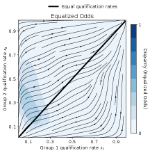
Our experiments show that algorithms trained with an RL formulation of long-term fairness can drive a reactive population toward states with higher utility and fairness, even when short-term utility is misaligned with desirable dynamics. Our central hypothesis, that long-term fairness via RL may induce an algorithm to sacrifice short-term utility for better long-term outcomes, is concretely demonstrated by Fig. 1, in which a greedy classifier and L-UCBFair, maximizing true positive rate tp (Section 5.1) subject to demographic parity DP (Section 5.1), drive a population to universal non-qualification ( $\Pr(Y{=}1)\to 0)$ and universal qualification ( $\Pr(Y{=}1)\to 1)$ , respectively. Each phase plot shows the dynamics of qualification rates $q_{g}=\Pr(Y{=}1\mid G{=}g)$ , which parameterize the population state $s$ and define the axes, with streamlines; color depicts averaged disparity $\mathscr{D}$ incurred by $a$ in state $s$ .

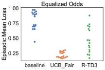
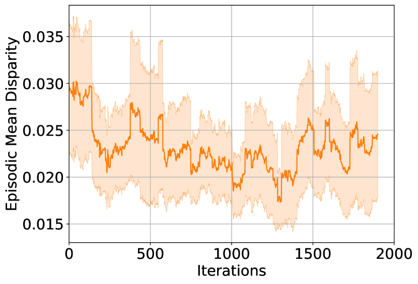
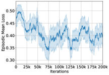
While both algorithms achieve no or little violation of demographic parity, the myopic algorithm eventually precludes future true-positive classifications (arrows in Fig. 1 approach a low qualification state), while L-UCBFair maintains stochastic thresholds at equilibrium (mean [0.49, 0.38], by group) with a non-trivial fraction of true-positives. The episodic mean loss and disparity training curves for L-UCBFair are depicted in Fig. 3.

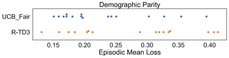
We show that RL algorithms that are not limited by the same restrictive assumptions as L-UCBFair are applicable to long-term fairness. In Fig. 2, R-TD3 achieves similar qualitative behavior (i.e., driving near-universal qualification at the expense of short-term utility) when optimizing a loss subject to scheduled disparity regularization. This figure also highlights the lack of guarantees of R-TD3 in incurring prominent violations of the fairness constraint and failing to convincingly asymptote to the global optimum.

Finally, we demonstrate the capability of RL to utilize notions of fairness that are impossible to treat in the myopic setting, viz. qualification rate parity, in Fig. 4. In this example, while both RL agents achieve qualification rate parity, we note that L-UCBFair fails to realize the optimal equilibrium discovered by R-TD3.

Concluding remarks

We have demonstrated that desirable social outcomes that are in conflict with myopic optimization may be realized as solutions to long-term fairness formalized through the lens of reinforcement learning. Moreover, we have shown that this problem both admits solutions with theoretical guarantees and can be relaxed to accommodate a wider class of recent advances in RL. We hope our contributions spur interest in long-term mechanisms and incentive structures for machine learning to be a driver of positive social change.

Acknowledgement

This work is partially supported by the National Science Foundation (NSF) under grants IIS-2143895 and IIS-2040800, and CCF-2023495.

References

Auer et al. (2002) Peter Auer, Nicolo Cesa-Bianchi, and Paul Fischer. Finite-time analysis of the multiarmed bandit problem. Machine learning, 47(2):235–256, 2002.
Bai et al. (2022) Qinbo Bai, Amrit Singh Bedi, Mridul Agarwal, Alec Koppel, and Vaneet Aggarwal. Achieving zero constraint violation for constrained reinforcement learning via primal-dual approach. In Proceedings of the AAAI Conference on Artificial Intelligence, volume 36, pages 3682–3689, 2022.
Brantley et al. (2020) Kianté Brantley, Miro Dudik, Thodoris Lykouris, Sobhan Miryoosefi, Max Simchowitz, Aleksandrs Slivkins, and Wen Sun. Constrained episodic reinforcement learning in concave-convex and knapsack settings. Advances in Neural Information Processing Systems, 33:16315–16326, 2020.
Brunton et al. (2021) Steven L Brunton, Marko Budišić, Eurika Kaiser, and J Nathan Kutz. Modern koopman theory for dynamical systems. arXiv preprint arXiv:2102.12086, 2021.
Chaney et al. (2018) Allison JB Chaney, Brandon M Stewart, and Barbara E Engelhardt. How algorithmic confounding in recommendation systems increases homogeneity and decreases utility. In Proceedings of the 12th ACM Conference on Recommender Systems, pages 224–232. ACM, 2018.
Chen et al. (2022) Yatong Chen, Reilly Raab, Jialu Wang, and Yang Liu. Fairness transferability subject to bounded distribution shift. arXiv preprint arXiv:2206.00129, 2022.
Coate and Loury (1993) Stephen Coate and Glenn C Loury. Will affirmative-action policies eliminate negative stereotypes? The American Economic Review, pages 1220–1240, 1993.
Crawford and Calo (2016) Kate Crawford and Ryan Calo. There is a blind spot in AI research. Nature News, 538(7625):311, 2016.
D’Amour et al. (2020) Alexander D’Amour, Hansa Srinivasan, James Atwood, Pallavi Baljekar, D Sculley, and Yoni Halpern. Fairness is not static: Deeper understanding of long term fairness via simulation studies. In Proceedings of the 2020 Conference on Fairness, Accountability, and Transparency, pages 525–534, 2020.
Ding et al. (2020) Dongsheng Ding, Kaiqing Zhang, Tamer Basar, and Mihailo Jovanovic. Natural policy gradient primal-dual method for constrained markov decision processes. Advances in Neural Information Processing Systems, 33:8378–8390, 2020.
Ding et al. (2021) Dongsheng Ding, Xiaohan Wei, Zhuoran Yang, Zhaoran Wang, and Mihailo Jovanovic. Provably efficient safe exploration via primal-dual policy optimization. In International Conference on Artificial Intelligence and Statistics, pages 3304–3312. PMLR, 2021.
Dua and Graff (2017) Dheeru Dua and Casey Graff. UCI machine learning repository, 2017. URL http://archive.ics.uci.edu/ml.
Dwork et al. (2012) Cynthia Dwork, Moritz Hardt, Toniann Pitassi, Omer Reingold, and Richard Zemel. Fairness through awareness. In Proceedings of the 3rd innovations in theoretical computer science conference, pages 214–226, 2012.
Efroni et al. (2020) Yonathan Efroni, Shie Mannor, and Matteo Pirotta. Exploration-exploitation in constrained mdps. arXiv preprint arXiv:2003.02189, 2020.
Ensign et al. (2018) Danielle Ensign, Sorelle A Friedler, Scott Neville, Carlos Scheidegger, and Suresh Venkatasubramanian. Runaway feedback loops in predictive policing. In Conference of Fairness, Accountability, and Transparency, 2018.
Epasto et al. (2020) Alessandro Epasto, Mohammad Mahdian, Vahab Mirrokni, and Emmanouil Zampetakis. Optimal approximation-smoothness tradeoffs for soft-max functions. Advances in Neural Information Processing Systems, 33:2651–2660, 2020.
Feldman et al. (2015) Michael Feldman, Sorelle A Friedler, John Moeller, Carlos Scheidegger, and Suresh Venkatasubramanian. Certifying and removing disparate impact. In proceedings of the 21th ACM SIGKDD international conference on knowledge discovery and data mining, pages 259–268, 2015.
Fujimoto et al. (2018) Scott Fujimoto, Herke Hoof, and David Meger. Addressing function approximation error in actor-critic methods. In International conference on machine learning, pages 1587–1596. PMLR, 2018.
Fuster et al. (2018) Andreas Fuster, Paul Goldsmith-Pinkham, Tarun Ramadorai, and Ansgar Walther. Predictably unequal? The effects of machine learning on credit markets. The Effects of Machine Learning on Credit Markets, 2018.
Ghosh et al. (2022) Arnob Ghosh, Xingyu Zhou, and Ness Shroff. Provably efficient model-free constrained rl with linear function approximation. arXiv preprint arXiv:2206.11889, 2022.
Hardt et al. (2016) Moritz Hardt, Eric Price, and Nathan Srebro. Equality of opportunity in supervised learning, 2016.
Heidari et al. (2019) Hoda Heidari, Vedant Nanda, and Krishna P. Gummadi. On the long-term impact of algorithmic decision policies: Effort unfairness and feature segregation through social learning. the International Conference on Machine Learning (ICML), 2019.
Hu and Chen (2018) Lily Hu and Yiling Chen. A short-term intervention for long-term fairness in the labor market. In Proceedings of the 2018 World Wide Web Conference on World Wide Web, pages 1389–1398. International World Wide Web Conferences Steering Committee, 2018.
Hu et al. (2019) Lily Hu, Nicole Immorlica, and Jennifer Wortman Vaughan. The disparate effects of strategic manipulation. In Proceedings of the Conference on Fairness, Accountability, and Transparency, pages 259–268, 2019.
Jabbari et al. (2017) Shahin Jabbari, Matthew Joseph, Michael Kearns, Jamie Morgenstern, and Aaron Roth. Fairness in reinforcement learning. In International conference on machine learning, pages 1617–1626. PMLR, 2017.
Jin et al. (2020) Chi Jin, Zhuoran Yang, Zhaoran Wang, and Michael I Jordan. Provably efficient reinforcement learning with linear function approximation. In Conference on Learning Theory, pages 2137–2143. PMLR, 2020.
Joseph et al. (2016) Matthew Joseph, Michael Kearns, Jamie H Morgenstern, and Aaron Roth. Fairness in learning: Classic and contextual bandits. Advances in neural information processing systems, 29, 2016.
Kalagarla et al. (2021) Krishna C Kalagarla, Rahul Jain, and Pierluigi Nuzzo. A sample-efficient algorithm for episodic finite-horizon mdp with constraints. In Proceedings of the AAAI Conference on Artificial Intelligence, volume 35, pages 8030–8037, 2021.
Liu et al. (2018) Lydia T Liu, Sarah Dean, Esther Rolf, Max Simchowitz, and Moritz Hardt. Delayed impact of fair machine learning. In International Conference on Machine Learning, pages 3150–3158. PMLR, 2018.
Liu et al. (2020) Lydia T Liu, Ashia Wilson, Nika Haghtalab, Adam Tauman Kalai, Christian Borgs, and Jennifer Chayes. The disparate equilibria of algorithmic decision making when individuals invest rationally. In Proceedings of the 2020 Conference on Fairness, Accountability, and Transparency, pages 381–391, 2020.
Liu et al. (2021) Tao Liu, Ruida Zhou, Dileep Kalathil, Panganamala Kumar, and Chao Tian. Learning policies with zero or bounded constraint violation for constrained mdps. Advances in Neural Information Processing Systems, 34:17183–17193, 2021.
Liu et al. (2017) Yang Liu, Goran Radanovic, Christos Dimitrakakis, Debmalya Mandal, and David C Parkes. Calibrated fairness in bandits. arXiv preprint arXiv:1707.01875, 2017.
Mouzannar et al. (2019) Hussein Mouzannar, Mesrob I Ohannessian, and Nathan Srebro. From fair decision making to social equality. In Proceedings of the Conference on Fairness, Accountability, and Transparency, pages 359–368. ACM, 2019.
Pan et al. (2019) Ling Pan, Qingpeng Cai, Qi Meng, Wei Chen, Longbo Huang, and Tie-Yan Liu. Reinforcement learning with dynamic boltzmann softmax updates. arXiv preprint arXiv:1903.05926, 2019.
Paszke et al. (2019) Adam Paszke, Sam Gross, Francisco Massa, Adam Lerer, James Bradbury, Gregory Chanan, Trevor Killeen, Zeming Lin, Natalia Gimelshein, Luca Antiga, Alban Desmaison, Andreas Kopf, Edward Yang, Zachary DeVito, Martin Raison, Alykhan Tejani, Sasank Chilamkurthy, Benoit Steiner, Lu Fang, Junjie Bai, and Soumith Chintala. Pytorch: An imperative style, high-performance deep learning library. In Advances in Neural Information Processing Systems 32, pages 8024–8035. Curran Associates, Inc., 2019.
Perdomo et al. (2020) Juan Perdomo, Tijana Zrnic, Celestine Mendler-Dünner, and Moritz Hardt. Performative prediction. In International Conference on Machine Learning, pages 7599–7609. PMLR, 2020.
Raab and Liu (2021) Reilly Raab and Yang Liu. Unintended selection: Persistent qualification rate disparities and interventions. Advances in Neural Information Processing Systems, 34:26053–26065, 2021.
Raffin et al. (2021) Antonin Raffin, Ashley Hill, Adam Gleave, Anssi Kanervisto, Maximilian Ernestus, and Noah Dormann. Stable-baselines3: Reliable reinforcement learning implementations. Journal of Machine Learning Research, 22(268):1–8, 2021.
Singh et al. (2020) Rahul Singh, Abhishek Gupta, and Ness B Shroff. Learning in markov decision processes under constraints. arXiv preprint arXiv:2002.12435, 2020.
Tang et al. (2021) Wei Tang, Chien-Ju Ho, and Yang Liu. Bandit learning with delayed impact of actions. Advances in Neural Information Processing Systems, 34:26804–26817, 2021.
Wei et al. (2022) Honghao Wei, Xin Liu, and Lei Ying. Triple-q: A model-free algorithm for constrained reinforcement learning with sublinear regret and zero constraint violation. In International Conference on Artificial Intelligence and Statistics, pages 3274–3307. PMLR, 2022.
Wen et al. (2019) Min Wen, Osbert Bastani, and Ufuk Topcu. Fairness with dynamics. arXiv preprint arXiv:1901.08568, 2019.
Williams and Kolter (2019) Joshua Williams and J Zico Kolter. Dynamic modeling and equilibria in fair decision making. arXiv preprint arXiv:1911.06837, 2019.
Xu et al. (2021) Tengyu Xu, Yingbin Liang, and Guanghui Lan. Crpo: A new approach for safe reinforcement learning with convergence guarantee. In International Conference on Machine Learning, pages 11480–11491. PMLR, 2021.
Zemel et al. (2013) Rich Zemel, Yu Wu, Kevin Swersky, Toni Pitassi, and Cynthia Dwork. Learning fair representations. In International conference on machine learning, pages 325–333. PMLR, 2013.
Zhang et al. (2020) Xueru Zhang, Ruibo Tu, Yang Liu, Mingyan Liu, Hedvig Kjellström, Kun Zhang, and Cheng Zhang. How do fair decisions fare in long-term qualification? arXiv preprint arXiv:2010.11300, 2020.
Zheng and Ratliff (2020) Liyuan Zheng and Lillian Ratliff. Constrained upper confidence reinforcement learning. In Learning for Dynamics and Control, pages 620–629. PMLR, 2020.

Appendix A Proof

Without loss of generality, we assume $\|\phi(s,a)\|\leq 1$ for all $(s,a)\in\mathcal{S}\times\mathcal{A}$ , and $\max\left\{\left\|\mu_{h}(\mathcal{S})\right\|,\left\|\theta_{h}\right\|\right\}\leq$ $\sqrt{d}$ for all $h\in[H]$ .

A.1 Proof of Theorem 3.7

See 3.7 Outline The outline of this proof simulates the proof in Ghosh et al. (2022). For brevity, denote $\mathbb{P}_{h}V_{j,h+1}^{\pi}(s,a)=\mathbb{E}_{s^{\prime}\sim\mathbb{P}_{h}(\cdot\mid s,a)}V_{j,h+1}^{\pi}\left(s^{\prime}\right)\text{ for }j=r,g$ . Then

	$\displaystyle Q_{j,h}^{\pi}(s,a)=\left(r_{h}+\mathbb{P}_{h}V_{j,h+1}^{\pi}\right)(s,a)$		(15)
	$\displaystyle V_{j,h}^{\pi}(s)=\left\langle\pi_{h}(\cdot\mid s)Q_{j,h}^{\pi}(s,\cdot)\right\rangle_{\mathcal{A}}$		(16)
	$\displaystyle\left\langle\pi_{h}(\cdot\mid s),Q_{j,h}^{\pi}(s,\cdot)\right\rangle_{\mathcal{A}}=\sum_{a\in\mathcal{A}}\pi_{h}(a\mid s)Q_{j,h}^{\pi}(s,a)$		(17)

Similar to Efroni et al. (2020), we establish

		$\displaystyle\text{Regret}(K)+\nu\text{Distortion}(K)$
	$\displaystyle=$	$\displaystyle\sum_{k=1}^{K}\left(V_{r,1}^{\pi^{*}}\left(s_{1}\right)-V_{r,1}^{\pi_{k}}\left(s_{1}\right)\right)+\nu\sum_{k=1}^{K}\left(b-V_{g,1}^{\pi_{k}}\left(s_{1}\right)\right)$
	$\displaystyle\leq$	$\displaystyle\underbrace{\sum_{k=1}^{K}\left(V_{r,1}^{\pi^{}}\left(s_{1}\right)+\nu_{k}V_{g,1}^{\pi^{}}\left(s_{1}\right)\right)-\left(V_{r,1}^{k}\left(s_{1}\right)+\nu_{k}V_{g,1}^{k}\left(s_{1}\right)\right)}_{\mathcal{T}_{1}}$
		$\displaystyle+\underbrace{\sum_{k=1}^{K}\left(V_{r,1}^{k}\left(s_{1}\right)-V_{r,1}^{\pi_{k}}\left(s_{1}\right)\right)+\nu\sum_{k=1}^{K}\left(V_{g,1}^{k}\left(s_{1}\right)-V_{g,1}^{\pi_{k}}\left(s_{1}\right)\right)}_{\mathcal{T}_{2}}$
		$\displaystyle+\underbrace{\frac{1}{2\eta}\nu^{2}+\frac{\eta}{2}H^{2}K}_{\mathcal{T}_{3}}$

$\mathcal{T}_{3}$ is easily bounded if $\eta$ . The major task remains bound $\mathcal{T}_{1}$ and $\mathcal{T}_{2}$ .

Bound $\mathcal{T}_{1}$ and $\mathcal{T}_{2}$ . We have following two lemmas.

Lemma A.1 (Boundedness of $\mathcal{T}_{1}$ ).

With probability $1-p/2$ , we have $\mathcal{T}_{1}\leq KH\left(\frac{\log(M)}{\alpha}+2(1+\mathscr{V})H\rho\epsilon_{I}\sqrt{\frac{dK}{\varsigma}}\right)$ . Specifically, if $\alpha=\frac{\log(M)K}{2(1+\mathscr{V}+H)}$ and $\varsigma=1$ , we have $\mathcal{T}_{1}\leq 2H(1+\mathscr{V}+H)+2KH^{2}(1+\mathscr{V})\rho\epsilon_{I}\sqrt{dK}$ with probability $1-p/2$ .

Lemma A.2 (Boundedness of $\mathcal{T}_{2}$ ).

Ghosh et al. (2022) With probability $1-p/2,\mathcal{T}_{2}\leq\mathcal{O}\left((\nu+1)H^{2}\zeta\sqrt{d^{3}K}\right)$ , where $\zeta=$ $\log[\log(M)4dHK/p]$ .

Lemma A.2 follows the same logic in Ghosh et al. (2022), and we delay the proof of Lemma A.1 to Section LABEL:sec:t1t2. Now we are ready to proof Theorem 3.7.

Proof.

For any $\nu\in[0,\mathscr{V}]$ , with prob. $1-p$ ,

	$\displaystyle\text{Regret}(K)+\nu\text{Distortion}(K)$
$\displaystyle\leq$	$\displaystyle\mathcal{T}_{1}+\mathcal{T}_{2}+\mathcal{T}_{3}$
$\displaystyle\leq$	$\displaystyle\frac{1}{2\eta}\nu^{2}+\frac{\eta}{2}H^{2}K+\frac{HK\log M}{\alpha}+2KH^{2}(1+\mathscr{V})\rho\epsilon_{I}\sqrt{dK}+\mathcal{O}\left((\nu+1)H^{2}\zeta\sqrt{d^{3}K}\right)$	(19)

Taking $\nu=0,\eta=\frac{\mathscr{V}}{\sqrt{KH^{2}}},\alpha=\frac{K\log M}{2(1+\mathscr{V}+H)},\epsilon_{I}=\frac{1}{2\rho(1+\mathscr{V})KH\sqrt{d}}$ , there exist constant $b$ ,

	$\displaystyle\text{Regret}(K)$	$\displaystyle\leq\frac{\mathscr{V}H}{2}\sqrt{K}+2H(1+\mathscr{V}+H)+2H^{2}K(1+\mathscr{V})\rho\epsilon_{I}\sqrt{dK}+\mathcal{O}\left(H^{2}\zeta\sqrt{d^{3}K}\right)$
		$\displaystyle\leq\big{(}b\zeta H^{2}\sqrt{d^{3}}+(\mathscr{V}+1)H\big{)}\sqrt{K}=\mathcal{\tilde{O}}(H^{2}\sqrt{d^{3}K}).$

Taking $\nu=\mathscr{V},\eta=\frac{\mathscr{V}}{\sqrt{KH^{2}}},\alpha=\frac{K\log M}{2(1+\mathscr{V}+H)},\epsilon_{I}=\frac{1}{2\rho(1+\mathscr{V})KH\sqrt{d}}$ ,

\displaystyle\text{Regret}(K)+\mathscr{V}\text{Distortion}(K)

\displaystyle\leq(\mathscr{V}+1)H\sqrt{K}+(1+\mathscr{V})\mathcal{O}\left(H^{2}\zeta\sqrt{d^{3}K}\right)

Following the idea of Efroni et al. (2020), there exists a policy $\pi^{\prime}$ such that $V_{r,1}^{\pi^{\prime}}=\frac{1}{K}\sum_{k=1}^{K}V_{r,1}^{\pi_{k}},V_{g,1}^{\pi^{\prime}}=\frac{1}{K}\sum_{k=1}^{K}V_{g,1}^{\pi_{k}}$ . By the occupancy measure, $V_{r,1}^{\pi}$ and $V_{g,1}^{\pi}$ are linear in occupancy measure induced by $\pi$ . Thus, the average of $K$ occupancy measure also produces an occupancy measure which induces policy $\pi^{\prime}$ and $V_{r,1}^{\pi^{\prime}}$ , and $V_{g,1}^{\pi^{\prime}}$ . We take $\nu=0$ when $\sum_{k=1}^{K}\left(b-V_{g,1}^{\pi_{k}}\left(s_{1}^{k}\right)\right)<0$ , otherwise $\nu=\mathscr{V}$ . Hence, we have

	$\displaystyle V_{r,1}^{\pi^{*}}\left(s_{1}\right)-\frac{1}{K}\sum_{k=1}^{K}V_{r,1}^{\pi_{k}}\left(s_{1}\right)+\mathscr{V}\max\big{(}(c-\frac{1}{K}\sum_{k=1}^{K}V_{g,1}^{\pi_{k}}\left(s_{1}\right),0\big{)}$
	$\displaystyle=V_{r,1}^{\pi^{*}}\left(s_{1}\right)-V_{r,1}^{\pi^{\prime}}\left(s_{1}\right)+\mathscr{V}\max\big{(}c-V_{g,1}^{\pi^{\prime}}\left(s_{1}\right),0\big{)}$
	$\displaystyle\leq\frac{\mathscr{V}+1}{K}H\sqrt{K}+\frac{\mathscr{V}+1}{K}\mathcal{O}\left(H^{2}\zeta\sqrt{d^{3}K}\right)$		(20)

Since $\mathscr{V}=2H/\gamma$ , and using the result of Lemma A.11, we have

\max\big{(}c-\frac{1}{K}\sum_{k=1}^{K}V_{g,1}^{\pi_{k}}\left(s_{1}^{k}\right),0\big{)}\leq\frac{\mathscr{V}+1}{K\mathscr{V}}\mathcal{O}\left(H^{2}\zeta\sqrt{d^{3}K}\right)

In this section we proof Lemma A.1 and Lemma A.2.

A.2 Prepare for Lemma A.1

In order to bound $\mathcal{T}_{1}$ and $\mathcal{T}_{2}$ , we introduce the following lemma.

Lemma A.3.

There exists a constant $B_{2}$ such that for any fixed $p\in(0,1)$ , with probability at least $1-p/2$ , the following event holds

\|\sum_{\tau=1}^{k-1}\phi_{j,h}^{\tau}\left[V_{j,h+1}^{k}\left(s_{h+1}^{\tau}\right)-\mathbb{P}_{h}V_{j,h+1}^{k}\left(s_{h}^{\tau},a_{h}^{\tau}\right)\|_{\left(\varsigma_{h}^{k}\right)^{-1}}\leq B_{2}dHq\right.

for $j\in\{r,g\}$ , where $q=\sqrt{\log\left[4\left(B_{1}+1\right)\log(M)dT/p\right]}$ for some constant $B_{1}$ .

We delay the proof of Lemma A.3 to Section A.4.

Lemma A.3 shows the bound of estimated value function $V^{k}_{j,h}$ and value function $V^{\pi}_{j,h}$ corresponding in a given policy at k. We now introcuce the following lemma appeared in Ghosh et al. (2022). This lemma bounds the difference between the value function without bonus in L-UCBFair and the true value function of any policy $\pi$ . This is bounded using their expected difference at next step, plus a error term.

Lemma A.4.

Ghosh et al. (2022) There exists an absolute constant $\beta=C_{1}dH\sqrt{\zeta},\zeta=\log(\log(M)4dT/p)$ , and for any fixed policy $\pi$ , for the event defined in Lemma A.3, we have

\left\langle\phi(s,a),w_{j,h}^{k}\right\rangle-Q_{j,h}^{\pi}(s,a)=\mathbb{P}_{h}\left(V_{j,h+1}^{k}-V_{j,h+1}^{\pi}\right)(s,a)+\Delta_{h}^{k}(s,a)

for some $\Delta_{h}^{k}(s,a)$ that satisfies $\left|\Delta_{h}^{k}(s,a)\right|\leq\beta\sqrt{\phi(s,a)^{T}\left(\Lambda_{h}^{k}\right)^{-1}\phi(s,a)}$ .

Lemma A.5.

Ghosh et al. (2022) With probability at least $1-p/2$ , (for the event defined in Lemma A.3)

Q_{r,h}^{\pi}(s,a)+\nu_{k}Q_{g,h}^{\pi}(s,a)\leq Q_{r,h}^{k}(s,a)+\nu_{k}Q_{g,h}^{k}(s,a)-\mathbb{P}_{h}\left(V_{h+1}^{k}-V_{h+1}^{\pi,\nu_{k}}\right)(s,a)

We also introduce the following lemma. This lemma bound the value function by taking L-UCBFair policy and greedy policy.

Lemma A.6.

Define $\bar{V}_{h}^{k}(\cdot)=\max_{a}\left[Q_{r,h}^{k}(\cdot,a)+\nu_{k}Q_{g,h}^{k}(\cdot,a)\right]$ the value function corresponding to greedy policy, we have

\bar{V}_{h}^{k}(s)-V_{h}^{k}(s)\leq\frac{\log M}{\alpha}+2(1+\mathscr{V})H\rho\epsilon_{I}\sqrt{\frac{dk}{\varsigma}}.

(21)

Proof.

Define $a_{g}$ the solution of greedy policy,

$\displaystyle V_{h}^{k}(s)-V_{h}^{k}(s)=$	$\displaystyle\left[Q_{r,h}^{k}\left(s,a_{g}\right)+\nu_{k}Q_{g,h}^{k}\left(s,a_{g}\right)\right]$	(22)
	$\displaystyle-\int_{a}\pi_{h,k}(a\mid s)\left[Q_{r,h}^{k}(s,a)+\nu_{k}Q_{g,h}^{k}(s,a)\right]da$	(23)
$\displaystyle\leq$	$\displaystyle\left[Q_{r,h}^{k}\left(s,a_{g}\right)+\nu_{k}Q_{g,h}^{k}\left(s,a_{g}\right)\right]$	(24)
	$\displaystyle-\sum_{i}\text{SM}_{\alpha}(I_{i}\mid x)\left[Q_{r,h}^{k}(x,I_{i})+\nu_{k}Q_{g,h}^{k}(x,I_{i})\right]+2(1+\mathscr{V})H\rho\epsilon_{I}\sqrt{\frac{dk}{\varsigma}}$	(25)
$\displaystyle\leq$	$\displaystyle\left(\frac{\log\left(\sum_{a}\exp\left(\alpha\left(Q_{r,h}^{k}(s,I_{i})+\nu_{k}Q_{g,h}^{k}(s,I_{i})\right)\right)\right)}{\alpha}\right)$	(26)
	$\displaystyle-\sum_{i}\text{SM}_{\alpha}(I_{i}\mid s)\left[Q_{r,h}^{k}(s,I_{i})+\nu_{k}Q_{g,h}^{k}(s,I_{i})\right]+2(1+\mathscr{V})H\rho\epsilon_{I}\sqrt{\frac{dk}{\varsigma}}$	(27)
$\displaystyle\leq$	$\displaystyle\frac{\log(M)}{\alpha}+2(1+\mathscr{V})H\rho\epsilon_{I}\sqrt{\frac{dk}{\varsigma}}.$	(28)

The first inequality follows from Lemma A.10 and the second inequality holds because of Proposition 1 in Pan et al. (2019).

A.3 Proof of Lemma A.1

Now we’re ready to proof Lemma A.1.

Proof.

This proof simulates Lemma 3 in Ghosh et al. (2022).

We use induction to proof this lemma. At step $H$ , we have $Q_{j,H+1}^{k}=0=Q_{j,H+1}^{\pi}$ by definition. Under the event in Lemma A.9 and using Lemma A.4, we have for $j=r,g$ ,

\left|\left\langle\phi(s,a),w_{j,H}^{k}(s,a)\right\rangle-Q_{j,H}^{\pi}(s,a)\right|\leq\beta\sqrt{\phi(s,a)^{T}\left(\Lambda_{H}^{k}\right)^{-1}\phi(s,a)}

Thus $Q_{j,H}^{\pi}(s,a)\leq\min\left\{\left\langle\phi(s,a),w_{j,H}^{k}\right\rangle+\beta\sqrt{\phi(s,a)^{T}\left(\Lambda_{H}^{k}\right)^{-1}\phi(s,a)},H\right\}=Q_{j,H}^{k}(s,a)$ .

From the definition of $\bar{V}_{h}^{k}$ ,

\bar{V}_{H}^{k}(s)=\max_{a}\left[Q_{r,H}^{k}(s,a)+\nu_{k}Q_{g,h}^{k}(s,a)\right]\geq\sum_{a}\pi(a\mid x)\left[Q_{r,H}^{\pi}(s,a)+\nu_{k}Q_{g,H}^{\pi}(s,a)\right]=V_{H}^{\pi,\nu_{k}}(s)

for any policy $\pi$ . Thus, it also holds for $\pi^{*}$ , the optimal policy. Using Lemma A.6 we can get

V_{H}^{\pi^{*},\nu_{k}}(s)-V_{H}^{k}(s)\leq\frac{\log M}{\alpha}+2(1+\mathscr{V})H\rho\epsilon_{I}\sqrt{\frac{dk}{\varsigma}}

Now, suppose that it is true till the step $h+1$ and consider the step $h$ . Since, it is true till step $h+1$ , thus, for any policy $\pi$ ,

\mathbb{P}_{h}\left(V_{h+1}^{\pi,\nu_{k}}-V_{h+1}^{k}\right)(s,a)\leq(H-h)\big{(}\frac{\log M}{\alpha}+2(1+\mathscr{V})H\rho\epsilon_{I}\sqrt{\frac{dk}{\varsigma}}\big{)}

From (27) in Lemma 10 and the above result, we have for any $(s,a)$

Q_{r,h}^{\pi}(s,a)+\nu_{k}Q_{g,h}^{\pi}(s,a)\leq Q_{r,h}^{k}(s,a)+\nu_{k}Q_{g,h}^{k}(s,a)+(H-h)\big{(}\frac{\log M}{\alpha}+2(1+\mathscr{V})H\rho\epsilon_{I}\sqrt{\frac{dk}{\varsigma}}\big{)}

Hence,

V_{h}^{\pi,\nu_{k}}(s)\leq\bar{V}_{h}^{k}(s)+(H-h)\big{(}\frac{\log M}{\alpha}+2(1+\mathscr{V})H\rho\epsilon_{I}\sqrt{\frac{dk}{\varsigma}}\big{)}

Now, again from Lemma 11, we have $\bar{V}_{h}^{k}(s)-V_{h}^{k}(s)\leq\frac{\log(|\mathcal{A}|)}{\alpha}$ . Thus,

V_{h}^{\pi,\nu_{k}}(s)-V_{h}^{k}(s)\leq(H-h+1)\big{(}\frac{\log M}{\alpha}+2(1+\mathscr{V})H\rho\epsilon_{I}\sqrt{\frac{dk}{\varsigma}}\big{)}

Now, since it is true for any policy $\pi$ , it will be true for $\pi^{*}$ . From the definition of $V^{\pi,\nu_{k}}$ , we have

\left(V_{r,h}^{\pi^{*}}(s)+\nu_{k}V_{g,h}^{\pi^{*}}(s)\right)-\left(V_{r,h}^{k}(s)+\nu_{k}V_{g,h}^{k}(s)\right)\leq(H-h+1)\big{(}\frac{\log M}{\alpha}+2(1+\mathscr{V})H\rho\epsilon_{I}\sqrt{\frac{dk}{\varsigma}}\big{)}

Hence, the result follows by summing over $K$ and considering $h=1$ .

A.4 Proof of Lemma A.3

We first define some useful sets. Let $\mathcal{Q}_{j}=\left\{Q\mid Q(\cdot,a)=\min\left\{w_{j}^{T}\phi(\cdot,a)+\beta\sqrt{\phi^{T}(\cdot,a)^{T}\Lambda^{-1}\phi(\cdot,a)},H\right\},\ a\in\mathcal{A}\right\}$ be the set of Q functions, where $j\in\{r,g\}$ . Since the minimum eigen value of $\Lambda$ is no smaller than one so the Frobenius norm of $\Lambda^{-1}$ is bounded.

Let $\mathcal{V}_{j}=\left\{V_{j}\mid V_{j}(\cdot)=\int_{a}\pi(a\mid\cdot)Q_{j}(\cdot,a)da;Q_{r}\in\mathcal{Q}_{r},Q_{g}\in\mathcal{Q}_{g},\nu\in[0,\mathscr{V}]\right\}$ be the set of Q functions, where $j\in\{r,g\}$ . Define

\Pi=\left\{\pi\mid\forall a\in\mathcal{A},\pi(a\mid\cdot)=\frac{1}{\int_{b\in\mathcal{I}(a)}db}\text{SM}_{\alpha}\left(Q_{r}(\cdot,I(a))+\nu Q_{g}(\cdot,I(a))\right),\ Q_{r}\in\mathcal{Q}_{r},Q_{g}\in\mathcal{Q}_{g},\nu\in[0,\mathscr{V}]\right\}

the set of policies.

It’s easy to verify $V_{j}^{k}\in\mathcal{V}_{j}$ .

Then we introduce the proof of Lemma A.3. To proof Lemma A.3, we need the $\epsilon$ -covering number for the set of value functions(Lemma A.9Ghosh et al. (2022)). To achieve this, we need to show if two $Q$ functions and the dual variable $\nu$ are close, then the bound of policy and value function can be derived(Lemma A.7, Lemma A.8). Though the proof of Lemma A.7 and Lemma A.8 are different from Ghosh et al. (2022), we show the results remain the same, thus Lemma A.9 still holds. We’ll only introduce Lemma A.9 and omit the proof.

We now proof Lemma A.7.

Lemma A.7.

Let $\pi$ be the policy of L-UCBFair corresponding to $Q^{k}_{r}+\nu_{k}Q^{k}_{g}$ , i.e.,

\pi(a\mid\cdot)=\frac{1}{\int_{b\in\mathcal{I}(a)}db}\text{SM}_{\alpha}\left(Q_{r}(\cdot,I(a))+\nu Q_{g}(\cdot,I(a))\right)

(29)

and

\tilde{\pi}(a\mid\cdot)=\frac{1}{\int_{b\in\mathcal{I}(a)}db}\text{SM}_{\alpha}\left(\tilde{Q}_{r}(\cdot,I(a))+\tilde{\nu}\tilde{Q}_{g}(\cdot,I(a))\right),

(30)

if $\left|Q_{j}-\tilde{Q}_{j}\right|\leq\epsilon^{\prime}$ and $\left|\nu-\tilde{\nu}\right|\leq\epsilon^{\prime}$ , then $\left|\int_{a}\left(\pi(a\mid x)-\tilde{\pi}(a\mid x)\right)da\right|\leq 2\alpha\epsilon^{\prime}(1+\mathscr{V}+H)$ .

Proof.

	$\displaystyle\left\|\int_{a}\left(\pi(a\mid x)-\tilde{\pi}(a\mid x)\right)da\right\|$	(31)
$\displaystyle=$	$\displaystyle\left\|\sum_{i=1}^{M}\int_{a\in\mathcal{I}_{i}}\left(\pi(I(a)\mid x)-\tilde{\pi}(I(a)\mid x)\right)da\right\|$
$\displaystyle=$	$\displaystyle\left\|\sum_{i=1}^{M}\int_{b\in\mathcal{I}_{i}}db\left(\pi(I_{i}\mid x)-\tilde{\pi}(I_{i}\mid x)\right)\right\|$
$\displaystyle\leq$	$\displaystyle\sum_{i=1}^{M}\left\|{SM}_{\alpha}\big{(}Q_{r}(s,I_{i})+\nu Q_{g}(s,I_{i})\big{)}-{SM}_{\alpha}\big{(}\tilde{Q}_{r}(s,I_{i})+\tilde{\nu}\tilde{Q}_{g}(s,I_{i})\big{)}\right\|$
$\displaystyle\leq$	$\displaystyle 2\alpha\left\|Q_{r}(\cdot,I(a))+\nu Q_{g}(\cdot,I(a))-\tilde{Q}_{r}(\cdot,I(a))-\tilde{\nu}\tilde{Q}_{g}(\cdot,I(a))\right\|$	(32)

The last inequaity holds because of Theorem 4.4 in Epasto et al. (2020). Using Corollary A.13, we have

\left|\int_{a}\left(\pi(a\mid x)-\tilde{\pi}(a\mid x)\right)da\right|\leq 2\alpha\epsilon^{\prime}(1+\mathscr{V}+H)

(33)

Now since we have Lemma A.7, we can further bound the value functions.

Lemma A.8.

If $\left|\tilde{Q}_{j}-Q_{j}^{k}\right|\leq\epsilon^{\prime}$ , where $\tilde{Q}_{j}\in\mathcal{Q}_{j}$ , then there exists $\tilde{V}_{j}\in\mathcal{V}_{j}$ such that

\left|V_{j}^{k}-\widetilde{V}_{j}\right|\leq H2\alpha\epsilon^{\prime}(1+\mathscr{V}+H)+\epsilon^{\prime},

Proof.

For any $x$ ,

		$\displaystyle V_{j}^{k}(s)-\widetilde{V}_{j}(s)$
		$\displaystyle=\left\|\int_{a}\pi(a\mid s)Q_{j}^{k}(s,a)da-\int_{a}\tilde{\pi}(a\mid s)\tilde{Q}_{j}(s,a)da\right\|$
		$\displaystyle=\left\|\int_{a}\pi(a\mid s)Q_{j}^{k}(s,a)da-\int_{a}\pi(a\mid s)\tilde{Q}_{j}(s,a)da+\int_{a}\pi(a\mid s)\tilde{Q}_{j}(s,a)da-\int_{a}\tilde{\pi}(a\mid s)\tilde{Q}_{j}(s,a)da\right\|$
		$\displaystyle\leq\left\|\int_{a}\pi(a\mid s)\left(Q_{j}^{k}(s,a)-\tilde{Q}_{j}(s,a)\right)da\right\|+\left\|\int_{a}\pi(a\mid s)\tilde{Q}_{j}(s,a)da-\int_{a}\tilde{\pi}(a\mid s)\tilde{Q}_{j}(s,a)da\right\|$
		$\displaystyle\leq\epsilon^{\prime}+H\left\|\int_{a}\left(\pi(a\mid s)-\tilde{\pi}(a\mid s)\right)da\right\|$
		$\displaystyle\leq\epsilon^{\prime}+H2\alpha\epsilon^{\prime}(1+\mathscr{V}+H)$

Using Lemmas above, we can have the same result presented in Lemma 13 of Ghosh et al. (2022) as following.

Lemma A.9.

Ghosh et al. (2022) There exists a $\tilde{V}_{j}\in\mathcal{V}_{j}$ parameterized by $\left(\tilde{w}_{r},\tilde{w}_{g},\tilde{\beta},\Lambda,\tilde{\mathscr{V}}\right)$ such that dist $\left(V_{j},\tilde{V}_{j}\right)\leq\epsilon$ where

\left|V_{j}-\tilde{V}_{j}\right|=\sup_{x}\left|V_{j}(s)-\tilde{V}_{r}(s)\right|.

Let $N_{\epsilon}^{V_{j}}$ be the $\epsilon$ -covering number for the set $\mathcal{V}_{j}$ , then,

\log N_{\epsilon}^{V_{j}}\leq d\log\left(1+8H\frac{\sqrt{dk}}{\sqrt{\varsigma}\epsilon^{\prime}}\right)+d^{2}\log\left[1+8d^{1/2}\beta^{2}/\left(\varsigma\left(\epsilon^{\prime}\right)^{2}\right)\right]+\log\left(1+\frac{\mathscr{V}}{\epsilon^{\prime}}\right)

where $\epsilon^{\prime}=\frac{\epsilon}{H2\alpha(1+\mathscr{V}+H)+1}$

Lemma A.10.

$|Q^{k}_{j,h}(s,a)-Q^{k}_{j,h}(s,I(a))|\leq 2H\rho\epsilon_{I}\sqrt{\frac{dK}{\varsigma}}$ .

Proof.

	$\displaystyle\Big{\|}Q^{k}_{j,h}(s,a)-Q^{k}_{j,h}(s,I(a))\Big{\|}$	(34)
$\displaystyle=$	$\displaystyle\Big{\|}w^{k}_{j,h}(s,a)^{T}(\phi(s,a)-\phi(s,I(a)))\Big{\|}$	(35)
$\displaystyle\leq$	$\displaystyle\|\|w^{k}_{j,h}(s,a)\\|_{2}\\|\phi(s,a)-\phi(s,I(a))\|\|_{2}$	(36)

From Lemma A.12 and 3.6 we get the result.

A.5 Preliminary Results

Lemma A.11.

Ding et al. (2021) Let $\nu^{*}$ be the optimal dual variable, and $C\geq 2\nu^{*}$ , then, if

V_{r,1}^{\pi^{*}}\left(s_{1}\right)-V_{r,1}^{\pi}\left(s_{1}\right)+C\left[c-V_{g,1}^{\pi}\left(s_{1}\right)\right]_{+}\leq\delta,

we have

\left[c-V_{g,1}^{\tilde{\pi}}\left(x_{1}\right)\right]_{+}\leq\frac{2\delta}{C}.

Lemma A.12.

Jin et al. (2020) For any $(k,h)$ , the weight $w_{j,h}^{k}$ satisfies

\left\|w_{j,h}^{k}\right\|\leq 2H\sqrt{dk/\varsigma}

Corollary A.13.

If $\operatorname{dist}\left(Q_{r},\tilde{Q}_{r}\right)\leq\epsilon^{\prime},\operatorname{dist}\left(Q_{g},\tilde{Q}_{g}\right)\leq\epsilon^{\prime}$ , and $\left|\tilde{\nu}_{k}-\nu_{k}\right|\leq\epsilon^{\prime}$ , then, $\operatorname{dist}\left(Q_{r}^{k}+\right.$ $\left.\nu_{k}Q_{g}^{k},\tilde{Q}_{r}+\tilde{\nu}_{k}\tilde{Q}_{g}\right)\leq\epsilon^{\prime}(1+\mathscr{V}+H)$ .

Appendix B Additional Figures

Appendix C Experiment

C.1 Experiment Details

Device and Packages. We run all the experiment on a single 1080Ti GPU. We implement the R-TD3 agent using StableBaseline3Raffin et al. (2021). The neural network is implemented using PytorchPaszke et al. (2019).

Neural Network to learn $\phi$ . We use a multi-layer perceptron to learn $\phi$ . Specifically, we sample 100000 data points using a random policy, storing $s$ , $a$ , $r$ and $g$ . The inputs of the network are state and action, passing through fully connected (fc) layers with size 256, 128, 64, 64. ReLU is used as activation function between fc layers, while a SoftMax layer is applied after the last fc layer. We treat the outcome of this network as $\phi$ . To learn $\phi$ , we apply two separated fc layers (without bias) with size 1 to $\hat{\phi}$ and treat the outputs as predicted $r$ and predicted $g$ . A combination of MSE losses of $r$ and $g$ are adopted. We use Adam as the optimizer. Weight decay is set to 1e-4 and learning rate is set to 1e-3, while batch size is 128.

Note that, $\hat{\phi}$ is linear regarding $r$ and $g$ , but the linearity of transition kernel cannot be captured using such a schema. Therefore, equivalently we made an assumption that there always exists measure $\mu_{h}$ such that for given $\hat{\phi}$ , the linearity of transition kernel holds. It’s a stronger assumption than Assumption 3.2.

		$\displaystyle V_{j}^{k}(s)-\widetilde{V}_{j}(s)$
		$\displaystyle=\left\|\int_{a}\pi(a\mid s)Q_{j}^{k}(s,a)da-\int_{a}\tilde{\pi}(a\mid s)\tilde{Q}_{j}(s,a)da\right\|$
		$\displaystyle=\left\|\int_{a}\pi(a\mid s)Q_{j}^{k}(s,a)da-\int_{a}\pi(a\mid s)\tilde{Q}_{j}(s,a)da+\int_{a}\pi(a\mid s)\tilde{Q}_{j}(s,a)da-\int_{a}\tilde{\pi}(a\mid s)\tilde{Q}_{j}(s,a)da\right\|$
		$\displaystyle\leq\left\|\int_{a}\pi(a\mid s)\left(Q_{j}^{k}(s,a)-\tilde{Q}_{j}(s,a)\right)da\right\|+\left\|\int_{a}\pi(a\mid s)\tilde{Q}_{j}(s,a)da-\int_{a}\tilde{\pi}(a\mid s)\tilde{Q}_{j}(s,a)da\right\|$
		$\displaystyle\leq\epsilon^{\prime}+H\left\|\int_{a}\left(\pi(a\mid s)-\tilde{\pi}(a\mid s)\right)da\right\|$
		$\displaystyle\leq\epsilon^{\prime}+H2\alpha\epsilon^{\prime}(1+\mathscr{V}+H)$

Long-Term Fairness with Unknown Dynamics

Abstract

1 Introduction

1.1 Related Work

2 Problem Formulation

State, Action, and Policy

Dynamics

Reward and Utility

Value and Quality Functions

“Long-term fairness” via reinforcement learning

Assumption 2.1 (Slater’s Condition).

The Online Setting

3 Algorithms and Analysis

3.1 L-UCBFair

Episodic MDP

Episodic Regret

The Lagrangian

Lemma 3.1 (Boundedness of ν∗\nu^{*}).

Assumption 3.2 (Linear MDP).

3.1.1 Explicit Construction

LSVI-UCB Jin et al. (2020)

Definition 3.3.

Lemma 3.4.

Theorem 3.5.

Assumption 3.6.

3.1.2 Analysis

Theorem 3.7 (Boundedness).

3.2 R-TD3

3.3 Greedy Baseline

4 Simulated Environments

4.1 Setting

Assumption 4.1 (Well-behaved feature).

Theorem 4.2 (Threshold Bayes-optimality).

4.2 Replicator Dynamics

4.3 Data Synthesis and Processing

4.4 Linearity of Dynamics

5 Experimental Results

5.1 Losses and Disparities Considered

5.2 Results

Concluding remarks

Acknowledgement

References

Appendix A Proof

A.1 Proof of Theorem 3.7

Lemma A.1 (Boundedness of 𝒯1\mathcal{T}_{1}).

Lemma A.2 (Boundedness of 𝒯2\mathcal{T}_{2}).

Proof.

A.2 Prepare for Lemma A.1

Lemma A.3.

Lemma A.4.

Lemma A.5.

Lemma A.6.

Proof.

A.3 Proof of Lemma A.1

Proof.

A.4 Proof of Lemma A.3

Lemma A.7.

Proof.

Lemma A.8.

Proof.

Lemma A.9.

Lemma A.10.

Proof.

A.5 Preliminary Results

Lemma A.11.

Lemma A.12.

Corollary A.13.

Appendix B Additional Figures

Appendix C Experiment

C.1 Experiment Details

C.2 zero one accuracy with more weights on true positive

C.3 Training Curves: L-UCBFair

C.3.1

C.4 Training Curves: R-TD3

C.5 Reduction of Utility

Lemma 3.1 (Boundedness of $\nu^{*}$ ).

Lemma A.1 (Boundedness of $\mathcal{T}_{1}$ ).

Lemma A.2 (Boundedness of $\mathcal{T}_{2}$ ).