Long-Pulse Laser-Induced Cavitation: A Race Between Advection and Phase Transition
Abstract
Vapor bubbles generated by long-pulsed laser often have complex non-spherical shapes that reflect some characteristics (e.g., direction, width) of the laser beam. The transition between two commonly observed shapes — namely, a rounded pear-like shape and an elongated conical shape — is studied using a new computational model that combines compressible multiphase fluid dynamics with laser radiation and phase transition. Two laboratory experiments are simulated, in which Holmium:YAG and Thulium fiber lasers are used separately to generate bubbles of different shapes. In both cases, the bubble morphology predicted by the simulation agrees reasonably well with the experimental measurement. The simulated laser radiance, temperature, velocity, and pressure fields are analyzed to explain bubble dynamics and energy transmission. It is found that due to the lasting energy input (i.e. long-pulsed laser), the vapor bubble’s dynamics is driven not only by advection, but also by the continuation of vaporization. Notably, vaporization lasts less than microsecond in the case of the pear-shaped bubble, versus more than microseconds for the elongated bubble. It is hypothesized that the bubble’s shape is the result of a competition. When the speed of advection is higher than that of vaporization, the bubble tends to grow spherically. Otherwise, it elongates along the laser beam direction. To clarify and test this hypothesis, the two speeds are defined analytically using a simplified model, then estimated for the experiments using simulation results. The results support the hypothesis. They also suggest that a higher laser absorption coefficient and a narrower beam facilitate bubble elongation.
1 Introduction
Vapor bubbles appear in many scientific studies and real-world applications that involve laser radiation. To researchers who study cavitation and bubble dynamics, laser is a convenient tool to create bubbles at a precise location without too much disturbance to the surrounding environment (Zwaan et al., 2007; Tomita et al., 2002; Brujan et al., 2001). To technology developers and practitioners who use high-power laser in a liquid environment, cavitation is often an inevitable phenomenon, and the resulting vapor bubbles may have both beneficial and detrimental effects. Example applications in this regard include liquid-assisted laser processing (e.g., underwater laser cutting (Chida et al., 2003), laser cleaning (Ohl et al., 2006; Song et al., 2004)), ocular laser surgery (Vogel et al., 1986; Požar et al., 2020), laser angioplasty (Vogel et al., 1996), and laser lithotripsy (Fried & Irby, 2018; Ho et al., 2021). The most common effects of laser-induced cavitation include the creation of a vapor channel, the disturbance of the local flow field, a propulsive force from bubble expansion, and material damages caused by the shock waves and micro-jets from bubble collapse (Chen et al., 2022; Xiang et al., 2023; Dijkink & Ohl, 2008; Mohammadzadeh et al., 2015). Improving a technology often requires optimizing the trade-offs between these effects.
While laser-induced cavitation can be roughly described as localized boiling through thermal radiation, the detailed physics involves laser emission and absorption, phase transition, and the dynamics and thermodynamics of a two-phase fluid flow. Within this multiphysics problem, a key external (i.e. user-specified) parameter is the duration of the laser pulse. In different applications, the value of this parameter varies from femtoseconds ( s) to more than one second (Zwaan et al., 2007; Ho et al., 2021; Juhasz et al., 1996). When the pulse duration is much smaller than the acoustic time scale in the fluid medium (i.e., characteristic length divided by sound speed), the laser energy input is referred to as short-pulsed. In this case, laser radiation can be assumed to be a preceding event that ends before the vapor bubble starts to expand. Therefore, the analysis of fluid and bubble dynamics can be separated from that of laser radiation, which simplifies the problem (Zein et al., 2013; Koch et al., 2016; Byun & Kwak, 2004). In this paper, we study cavitation induced by long-pulsed laser, which means the duration of the laser pulse is comparable to or longer than the acoustic time scale. In this case, laser radiation may continue after the formation of the initial bubble. The assumption mentioned above is no longer valid. Laser radiation, phase transition, and the fluid dynamics and thermodynamics are now interdependent. They need to be analyzed together.
The vapor bubbles generated by long-pulsed laser often have a non-spherical shape that reflects some characteristics of the laser beam, such as its direction and width. Figure 1 shows two commonly observed shapes that will be studied in this paper, namely a rounded pear-like shape and an elongated conical shape. Depending on the application, one or the other may be preferred. For example, a rounded bubble, when collapses, is more likely to generate a strong liquid jet that damages a surrounding material (Xiang et al., 2023; Chen et al., 2022). An elongated bubble, on the other hand, can be more energy efficient in creating a long vapor channel that allows laser to pass through. While bubbles of both shapes have been observed in many experiments (Mohammadzadeh et al., 2015; Hardy et al., 2016; Fried & Irby, 2018; Xiang et al., 2023), the causal relation between bubble morphology and laser setting (e.g., wavelength, power magnitude and distribution, pulse duration, diverging angle) is still unclear. Many fundamental questions of practical significance are unresolved, such as the following.
-
•
Does phase transition (vaporization) last for a substantial period of time, or does it occur instantaneously?
-
•
What fraction of the laser energy input is used to create the vapor bubble?
-
•
How to control the laser setting so that the vapor bubble has a desired shape?

It is difficult to answer these questions by laboratory experiment only. Some parameters of laser (e.g., wavelength) cannot be continuously varied in experiments. While the evolution of bubble shape can be measured by high-speed optical imaging, measurement of the pressure, velocity, and temperature fields inside and around the vapor bubble is challenging to say the least (Dular & Coutier-Delgosha, 2013; Petkovšek & Dular, 2013; Khlifa et al., 2013). Therefore, the partition of energy and the cause of the bubble’s shape change cannot be easily determined. In this work, we combine laboratory experiment with numerical simulation to study long-pulse laser-induced cavitation, focusing on the physics behind pear-shaped and elongated bubbles. We try to investigate the causal relation between laser setting and the vapor bubble’s shape, and to gain some insight on the three open questions mentioned above.
A key novelty in this work is the use of a new computational model that combines compressible multiphase fluid dynamics with laser radiation and phase transition. In the past, bubble dynamics simulations were typically based on the solution of Rayleigh-Plesset, boundary integral, or multi-dimensional Navier-Stokes equations (Warnez & Johnsen, 2015; Klaseboer et al., 2006; Wang, 2017; Cao et al., 2021a). Thermal radiation and the resulting phase transition were not included. A simulation usually starts with one or multiple spherical bubbles as the initial condition. In most cases, the initial state inside each bubble is set to a constant. This approach can be justified for bubbles generated by short-pulsed laser, given that radiation and vaporization both complete at a smaller time scale compared to that of fluid dynamics. For long-pulse laser-induced cavitation, the same approach is no longer valid. It would not be able to predict the effects of the lasting energy input, such as the possible continuation of phase transition and the formation of non-spherical bubbles. In this work, we couple the multiphase compressible inviscid Navier-Stokes equations with a laser radiation equation that models the absorption of laser by the fluid flow. The laser radiation equation is obtained by customizing the radiative transfer equation (RTE) using the special properties of laser, including monochromaticity, directionality, and a measurable (often non-zero) focusing or diverging angle. The key components of the computational framework include an embedded boundary method that allows the solution of laser and fluid governing equations on the same mesh, a method of latent heat reservoir for vaporization prediction, a local level set method for interface tracking, and the FIVER (FInite Volume method with Exact multi-material Riemann solvers) method to enforce interface conditions. The algorithms and properties of this framework were recently published in the Journal of Computational Physics, together with some verification tests (Zhao et al., 2023). The FIVER method by itself is the pivot of a body of literature that includes numerical method development, verification and validation, and various applications in aerospace, ocean, and biomedical engineering (Farhat et al. (2012); Main et al. (2017); Ma et al. (2023); Islam et al. (2023); Huang et al. (2018), and the references therein). Compared to the physical model presented in Zhao et al. (2023), a few improvements are made in this work, such as the inclusion of heat diffusion and the modeling of laser fiber using an embedded boundary method.
In two separate laboratory experiments, we use Holmium:Yttrium-Aluminum-Garnet (Ho:YAG) and Thulium fiber lasers to generate a pear-shaped bubble and an elongated bubble. In both cases, the bubble dynamics is recorded by high-speed optical imaging. In addition, the temporal profile of laser power is measured using a light detector. These experimental measurements are treated as ground truth in this study. We simulate the two experiments using the computational model described above. The measured laser power profile is used as an input to each simulation, which starts with a single phase (liquid water) in the entire computational domain. The simulations are capable of predicting bubble nucleation due to laser radiation. They provide transient, full-field results of laser radiance, temperature, pressure, velocity, and density. They also track the dynamics of the vapor bubble using a level set function. To validate the computational model, we compare the bubble dynamics predicted by the simulations with the high-speed images obtained from the experiments. Then, we analyze the full-field simulation results to explain the bubble dynamics and energy transmission. Based on the results, we hypothesize that the bubble’s shape is determined by a race between advection and phase transition. At any time instant, if the speed of advection is higher than that of vaporization, the bubble tends to grow spherically. Otherwise, it tends to elongate along the laser beam direction. To clarify this hypothesis, we build a simplified model problem for which the aformentioned two speeds can be analytically defined. Then, we test the hypothesis using our simulation results.
The remainder of this paper in organized as follows. Section 2 describes the physical model adopted in this study, including governing equations, constitutive models, and a phase transition model. Section 3 provides a summary of the numerical methods used to solve the model equations. In Sections 4 and 5, we present the experimental and simulation results for a pear-shaped bubble and an elongated bubble. In Section 6, we discuss the transition between these two different shapes. Finally, Section 7 provides a summary of this study and some concluding remarks.
2 Physical model
2.1 Fluid dynamics and thermodynamics
Figure 2 illustrates the problem investigated in this paper, showing a test case that generates a pear-shaped vapor bubble. The computational analysis is designed to start at the time when laser is just activated. At this time, the fluid domain is completely occupied by liquid water. The analysis is expected to predict the localized water vaporization due to laser radiation, the subsequent bubble and fluid dynamics, and the dissipation of laser energy in this two-phase fluid medium. Therefore, we solve the following compressible inviscid Navier-Stokes equations that include radiative heat transfer.
| (1) |
with
| (2) |

Here, denotes the domain of the fluid flow. Open subsets and represent the subdomains occupied by the liquid and vapor phases, respectively. They are time-dependent. In most experiments, a sharp boundary between the liquid and vapor phases can be clearly captured by high-speed cameras. Therefore, we assume . , , , and denote the fluid’s density, velocity, pressure, and temperature, respectively. is the total energy per unit mass, given by
| (3) |
where denotes the fluid’s internal energy per unit mass. is the thermal conductivity coefficient, which takes different values in and . denotes the radiative heat flux induced by laser. Equation (1) needs to be closed by a complete equation of state (EOS) for each phase, including a temperature equation. The computational model and solver utilized in this study supports arbitrary convex EOS (Ma et al., 2023). In this study, we adopt the Noble-Abel stiffened gas equation (Le Métayer & Saurel, 2016) for both phases. Specifically,
| (4) |
in which the subscript identifies the liquid () and vapor () phases. For each phase, , , , and are constant parameters that characterize its thermodynamic properties. For example, a non-zero allows the model to have a variable Grüneisen parameter that depends on . Clearly, (4) is a generalization of perfect gas, stiffened gas, and Noble-Abel equations of state (Le Métayer & Saurel, 2016).
For a given pressure equation like (4), the choice of temperature equation is not unique. We adopt the one proposed in Le Métayer & Saurel (2016), i.e.,
| (5) |
where denotes the specific heat capacity at constant volume, assumed to be a constant. It can be shown that the specific heat capacity at constant pressure, , is also a constant, given by . Combining (4) and (5) gives a complete EOS that satisfies the first law of thermodynamics.
Two groups of EOS parameter values are tested in this study, as shown in Table 1. Neither of them was calibrated specifically for laser-induced cavitation (Le Métayer & Saurel, 2016; Zein et al., 2013, see). We will show in Section 4 that the simulation result is indeed influenced by these parameter values.
| Group | Reference | Phase | |||||
|---|---|---|---|---|---|---|---|
| 1 | Zein et al. | Liquid | 2.057 | 1.066 | 3.449 | 0 | -1994.674 |
| (2013) | Vapor | 1.327 | 0 | 1.2 | 0 | 1995 | |
| 2 | Métayer et al. | Liquid | 1.19 | 7.028 | 4.285 | 6.61 | -1177.788 |
| (2016) | Vapor | 1.47 | 0 | 0.955 | 0 | 2077.616 |
2.2 Liquid-vapor interface
We model the bubble surface as a sharp interface with zero thickness. It is defined by
| (6) |
On the interface, we assume continuity of normal velocity and pressure, i.e.
| (7) |
where denotes the normal to .
is time-dependent, and must be solved for during the analysis. We represent it implicitly as the zero level set of a signed distance function, , defined in the closure of . That is,
| (8) |
where denotes the closure of .
In this way, the aforementioned phase identifier, , is given by
| (9) |
The evolution of in time is driven by both phase transition and advection. The advection of by the fluid flow is governed by the level-set equation,
| (10) |
where is the flow velocity.
2.3 Laser radiation
Let denote the region in the fluid domain that is exposed to laser. The laser generators used in this study have a flat surface with a small diverging angle. Therefore, is in the shape of a truncated cone (Fig. 2). Within , energy conservation implies
| (11) |
where denotes the spectral radiance (dimension: [mass][time]-3[length]-1) at position , along direction , at wavelength . and denote the coefficients of absorption and scattering, respectively. They depend on the laser’s wavelength and the medium. denotes the blackbody radiance. is the scattering phase function, which gives the probability that a ray from one direction would be scattered into another direction . If is independent of , the left-hand side of Eq. (11) simplifies to , which gives the well-known radiative transfer equation (RTE) (Modest, 2013; Howell et al., 2020).
The radiative heat flux in Eq. (1) is obtained by integrating over all directions and the interval of relevant wavelengths, . That is,
| (12) |
The special properties of laser light allows us to simplify (11) and (12). The intensity of the laser light is much higher than the blackbody radiance. Therefore, we assume
| (13) |
Also, is non-zero only along the direction of laser propagation () and at the fixed laser wavelength. That is,
| (14) |
where denotes the delta function, and the variable on the right-hand side is radiance (dimension: [mass][time]-3). With these assumptions, a laser radiation equation is obtained by substituting Eq. (14) and Eq. (13) into Eq. (11), i.e.,
| (15) |
Here, is a known function, but not a constant unless the laser light has a parallel beam. Similarly, substituting Eq. (14) into Eq. (12) yields
| (16) |
In this study, we measure the time history of laser power, , in laboratory experiments. We assume the laser radiance on the surface of the laser fiber (i.e., in Fig. 2) follows a Gaussian distribution, also known as a Gaussian beam (Welch et al., 2011). Therefore, on we have
| (17) |
where denotes the center of , and is the waist radius. (17) serves as a Dirichlet boundary condition for the laser radiation equation, (15).
2.4 Phase transition
We employ the method of latent heat reservoir proposed in Zhao et al. (2023) to predict laser-induced vaporization. As shown in Fig. 3, the fundamental idea of this method is to introduce a new variable, , to track the intermolecular potential energy in the liquid phase. The vaporization temperature, , and latent heat, , are assumed to be constant and used in the method as coefficients. When the analysis starts, is initialized to everywhere. As the liquid absorbs laser energy, temperature increases gradually. At any point , once is reached, additional heat — due to radiation, advection, or diffusion — is added to . When reaches , phase transition occurs. In Fig. 3, this time instant is denoted by . We assume that phase transition completes instantaneously at each point through an isochoric process. The state variables after phase transition are given by

| (18) | ||||
| (19) | ||||
| (20) | ||||
| (21) | ||||
| (22) |
where the superscripts and indicate the variable’s value before and after phase transition, e.g.,
| (23) |
In (22), denotes the local element size in the computational mesh. The pressure and temperature after phase transition are obtained naturally from the EOS of the vapor phase, i.e.,
| (24) | ||||
| (25) |
The pressure rise, , drives the expansion of the vapor bubble.
At each time step, if phase transition occurs, the level set function is restored to a signed distance function by solving the reinitialization equation,
| (26) |
to the steady state. Here, is a fictitious time variable. is the level set function before reinitialization. is a smoothed sign function, given by
| (27) |
where is a constant coefficient, set to the minimum element size of the mesh. The steady state solution of Eq. (26) is then used as the new initial condition to integrate the level set equation (10) forward in time.
3 Numerical methods
3.1 FIVER (FInite Volume method based on Exact multiphase Riemann problem solvers)
We apply a recently developed laser-fluid computational framework to solve the above model equations (Zhao et al., 2023). The fluid governing equations are semi-discretized using a fixed, non-interface conforming finite volume mesh, denoted by (Fig. 4). The laser fiber is modeled as a fixed slip wall, and the associated boundary condition is enforced using an embedded boundary method (Cao et al., 2018, 2021b; Wang, 2017; Cao et al., 2021a). Therefore, also covers the region occupied by the laser fiber. Around each node , a control volume is created. Applying the standard finite volume spatial discretization to Eq. (1) yields
| (28) |
where denotes the average value of in . denotes the set of nodes connected to node . . is the unit normal to . denotes the volume of .

The FIVER method is used to calculate the advective flux across each facet . Depending on the locations of nodes and , there are four different cases.
-
[(a)]
-
1.
If and belong to the same phase subdomain ( or ), the conventional monotonic upstream-centered scheme for conservation laws (MUSCL) is used to compute the flux across .
-
2.
If and belong to different phase subdomains, a one-dimensional bimaterial Riemann problem is constructed along the edge between and , i.e.,
(29) where denotes the time coordinate. denotes the spatial coordinate along the axis aligned with and centered at the phase interface between and . The initial state and are the projections of and on the axis. This 1D two-phase compressible flow problem can be solved exactly (Ma et al., 2023). The solution is self-similar, and satisfies the interface conditions (7). The states to the left and right of the interface are used in the numerical flux function to compute the advective fluxes across .
- 3.
-
4.
If both and are covered by the laser fiber, the flux across is set to zero.
3.2 Diffusive heat fluxes
The right-hand side of Eq. (28) includes two parts, namely the heat diffusion term () and the radiation term (). The heat diffusion term is evaluated using a finite volume method, i.e.
| (30) |
where is the area of facet . denotes the heat flow due to diffusion cross the facet . In this work, it is computed by
| (31) |
with
| (32) |
Here, and denote the thermal conductivity at nodes and , specifically. We assume that the liquid-vapor interface is isothermal, and it can be shown that if and belong to different phase subdomains, Eqs. (31) and (32) enforce energy balance at the interface, with interface temperature (Faghri & Zhang, 2006)
| (33) |
3.3 laser radiation and laser-fluid coupling
The radiation term is evaluated by
| (34) |
At each time step, the divergence of the radiative flux, , is computed using the current solution of the laser radiation equation (15). In this work, the laser radiation equation is discretized using the same finite volume mesh () created for the fluid governing equations (Fig. 4). Specifically, integrating (15) within an arbitrary cell yields
| (35) |
where is the cell-average of within . denotes the laser direction at , which is set to the laser direction at the midpoint between nodes and . is the value of at facet . In this work, it is evaluated by the mean flux method, i.e.
| (36) |
where is a numerical parameter. Substituting Eq. (36) into Eq. (35) yields a system of linear equations with the cell-averages of laser radiance as unknowns. The Gauss-Seidel method is applied to solve this system to get . Then, is obtained by
| (37) |
When solving the laser radiation equation, the fluid mesh does not contain a subset of nodes, edges, and elements that resolve the boundary of or the laser propagation directions . In this work, the embedded boundary method proposed in Zhao et al. (2023) is adopted to resolve this issue. This method involves the population of ghost nodes outside the side boundary of the laser domain using second-order mirroring and interpolation techniques.
The numerical methods described above are implemented in the M2C solver (Wang et al., 2021), which is used to run the simulations reported in this paper. Several verification studies can be found in Islam et al. (2023); Zhao et al. (2023); Cao et al. (2021a), and earlier papers cited therein. An outline of the solution procedure within each time step is provided below. For simplicity, the Forward Euler method is assumed here for time integration. In the actual simulations presented in this paper, a second-order Runge-Kutta method is used.
| Input: | Numerical solution at : , , , , and . | |
|---|---|---|
| (1) | Compute the residual of the Navier-Stokes equations (Eq. (28)). | |
| (1.1) | Compute the advective fluxes (Sec. 3.1). | |
| (1.2) | Compute the diffusive heat fluxes (Eq. (30)). | |
| (1.3) | Compute the radiative heat source (Eq. (34)). | |
| (2) | Advance the fluid state by one time step , . Apply boundary | |
| conditions. | ||
| (3) | Compute the residual of the level set equation (Eq. (10)). | |
| (4) | Advance the level set function by one time step . Apply boundary | |
| conditions. | ||
| (5) | Update phase identifier using . Update fluid state (, ) at | |
| nodes that changed phase due to interface motion. | ||
| (6) | Check for phase transition (Sec. 2.4). Update , , , and at | |
| nodes that have undergone phase transition (Eqs. (18)-(25)). | ||
| (7) | If phase transition occurred, reinitialize the level set equation (Eq. (26)). | |
| (8) | Solve the laser radiance equation for (Eq. (35)). | |
| Output: | Numerical solution at : , , , , and . | |
4 A pear-shaped bubble
We employ the computational framework described above to simulate a laboratory experiment that generates a pear-shaped bubble. The key parameters of the simulation, including laser fiber diameter, laser absorption coefficient, and the divergence angle of the laser beam, are set to match the setup of the experiment. The laser power used in the simulation (i.e. in Eq. (17) is determined by fitting the laser power profile measured in the experiment. The simulation’s output includes the time-histories of the density, temperature, pressure, velocity, and laser radiance fields of the two-phase flow, and the level-set function that tracks the liquid-vapor interface. The bubble’s nucleation and evolution are compared with high-speed optical images obtained from the experiment. By analyzing the full-field results obtained from the simulation, we try to investigate the causal relation between the laser setting and the bubble’s shape.
4.1 Comparison of experimental and numerical results
4.1.1 Laboratory experiment
In this experiment, a commercial Ho:YAG laser lithotripter (H Solvo -watt laser, Dornier MedTech, Munich, Germany) with a wavelength of is used to generate the vapor bubble. It is operated at the energy level of with a pulse duration of , measured at full width at half maximum. It is clearly a long-pulsed laser, as the acoustic time scale is less than . Figure 5(a) shows a schematic representation of the experimental setup. To facilitate the delivery of the pulsed laser, an optical fiber (Dornier SingleFlex , numerical aperture: , Munich, Germany) with a core diameter of is used. The fiber directs laser into a transparent acrylic container () filled with degassed water. During the experiment, a series of high-speed images are captured using an ultrahigh-speed camera. To enable direct shadowgraph imaging, a -ns pulsed laser system (SI-LUX-, Specialised Imaging) provides the required illumination.

To measure the laser power profile, an additional procedure is conducted in air. The laser pulse is directed towards a light detector (PDAD, Thorlabs, Newton, NJ) positioned at a distance of m, as illustrated in Fig. 5(b). The light detector converts the received light into an electronic signal, which is displayed on an oscilloscope. Since air has minimal absorption of laser energy, the recorded data can be considered a reliable indication of the laser power output from the laser fiber when generating the vapor bubble in the bulk fluid.
Figure 6(a) presents the time-history of the laser power measurement. The laser power increases from the beginning and reaches the maximum at approximately . After that, it gradually drops to zero. The graph reveals some fluctuations, which are attributed to measurement noise. Integrating the measured laser power in time yields a total pulse energy of J, which is in good agreement with the specified energy level. Figure 6(b) presents a series of high-speed images that show the nucleation and evolution of a vapor bubble at the tip of the laser fiber. The bubble becomes visible at . It expands continuously, eventually acquiring a pear-like shape. The bubble maintains cylindrical symmetry about the central axis of the laser beam. However, it is not spherical, unlike the bubbles obtained from previous experiments that use short-pulsed lasers (e.g., Brujan et al. (2001); Zhong et al. (2020); Lauterborn & Vogel (2013)).

Using the measured laser power profile, we can estimate the time it takes to heat water near the laser fiber tip to the vaporization temperature, . Here, we assume . We define a cylindrical region next to the laser fiber tip, with a diameter of (the laser fiber diameter) and a small depth of . The energy required to raise water temperature in this region from the room temperature (assumed to be ) to can be estimated by
| (38) |
with , and . The percentage of laser energy absorbed in this region can be roughly estimated by the Beer-Lambert law, which is the one-dimensional version of (15). That is,
| (39) |
The solution of this equation is simply , where denotes the laser radiance at the source (i.e., ). Setting for the Ho:YAG laser (Fried & Irby, 2018), we find that approximately of the laser energy is absorbed within the depth of the cylindrical region defined above. Now, by integrating the measured laser power profile (Fig. 6(a)), we can estimate that at approximately , the temperature within the small cylindrical region reaches . From the high-speed images, the vapor bubble does not appear until . This finding implies a clear delay in bubble nucleation, which can be attributed to the high latent heat of water.
4.1.2 Numerical simulation
Figure 7 shows the setup of the simulation. A cylindrical domain with a radius of mm and a length of mm is adopted. It is initially occupied by liquid water with density , velocity , pressure , and temperature .

The laser source is positioned at , as shown in Fig. 7(b). The laser fiber is modeled as a rigid structure, embedded in the computational domain. It has a radius , which is consistent with the laboratory experiment. The laser beam has a divergence angle , which depends on the numerical aperture (NA) of the fiber and the laser wavelength (Pal, 2010). The spatial profile of laser radiance on the source plane is specified as a Gaussian function (Eq. (17)) with waist radius , as shown in Fig. 7(c). The temporal profile of laser power () is specified as the blue line shown in Fig. 7(d). It is obtained by fitting the experimental measurement using fast Fourier transform (FFT). The pulse shape is approximately a triangle, with the power growing from to within , then vanishing gradually within . The laser absorption coefficient, , is set to for liquid water (Fried & Irby, 2018) and for the vapor. The vaporization temperature and latent heat of vaporization are set by and , respectively.
The Nobel-Abel stiffened gas EOS (Eq. (4)) is employed to model both liquid water and water vapor. First, we adopt the EOS parameters presented in Zein et al. (2013), which are listed as Group in Table 1. The thermal conductivity, , is set to for liquid water and (Wagner et al., 2010) for the vapor.
By the assumption of cylindrical symmetry, we solve the fluid governing equations on a two-dimensional mesh, while adding source terms to the equations to enforce the symmetry (see, e.g., Islam et al. (2023)). The mesh has approximately million rectangular elements. In the most refined area, the characteristic element size is about . To put this into context, the diameter of the laser fiber is resolved by about elements. The local level set method with a bandwidth of elements on each side of the interface is used to track the vapor bubble. Both the fluid governing equations and the level set equation are integrated in time using a second-order Runge-Kutta method. The time step size is approximately . The simulation is terminated at , which roughly covers the bubble nucleation and expansion stage observed in the laboratory experiment.
The simulation also generates a pear-shaped bubble, as observed in the experiment. Figure 8 presents a detailed comparison between the experimental data and the simulation result. In sub-figure (a), the high-speed images obtained from the experiment and the simulation results (bubble dynamics and laser radiance) are shown side by side. The simulation predicts that the vapor bubble nucleates at approximately . This is similar to the finding from the experiment, in which the bubble appears at . The overall bubble dynamics predicted by the simulation — that is, the evolution of the bubble’s size and overall shape — agrees reasonably well with the experimental data.
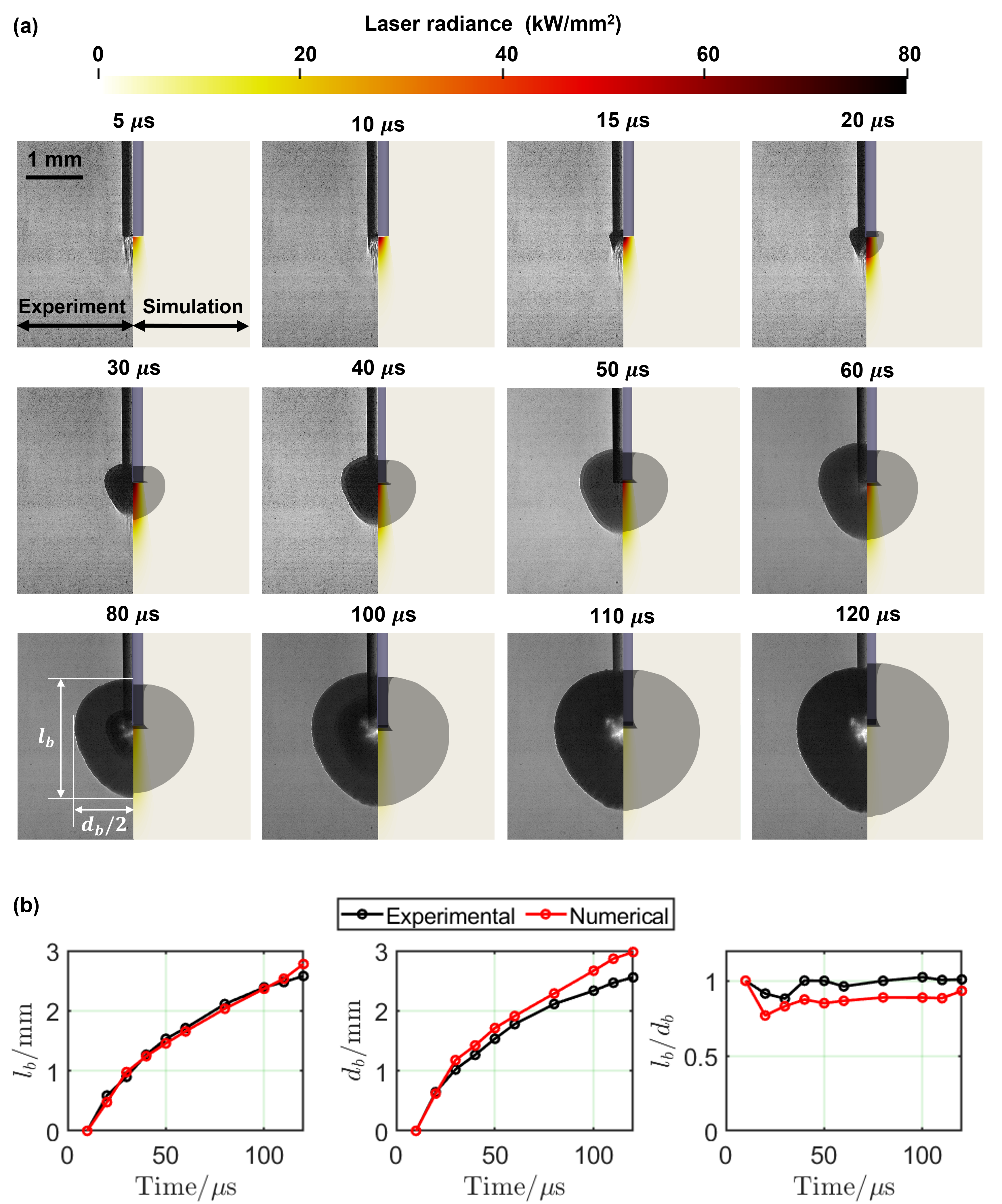
To make a quantitative comparison between the simulation result and the experimental data, we measure the maximum length of the bubble in two directions, that is, along and perpendicular to the laser fiber direction. These two measurements are denoted as and , respectively, and plotted in Fig. 8(b). The value of obtained from the simulation matches its experiment counterpart very well. The discrepancy between the simulation and the experiment in is a bit larger, between and at different time instants. Also, the bubble’s expansion speed in the perpendicular direction is slightly larger in the simulation than in the experiment. Furthermore, the aspect ratio of the bubble, defined as , is also calculated, and plotted in Fig. 8(b). In both the experiment and the simulation, it varies between and .
4.2 Delay of bubble nucleation due to latent heat
As mentioned in Sec. 4.1.1, the laboratory experiment reveals a delay of bubble nucleation, that is, the time of bubble nucleation is clearly after the time when the vaporization temperature () is reached at the fiber tip. The same phenomenon is observed in the simulation.
Figure 9 shows the temperature field at time instants during the early period of the simulation. At the beginning, the temperature of water in front of the laser fiber increases continuously, as it absorbs laser energy. This can be seen in the solution snapshots taken at to . At , the temperature of water next to the center of the fiber tip first reaches . This is about before bubble nucleation, which occurs at . Within this time period, the region that reaches expands continuously, but phase transition does not occur.

This time delay is due to the fact that water has a high latent heat of vaporization. Based on the values of and adopted in the simulation, the latent heat is about times the energy needed to raise water temperature from to . Using the phase transition model described in Sec. 2.4, as soon as is reached, any additional heat contributes towards increasing the intermolecular potential energy, thereby overcoming the required latent heat of vaporization. To examine this process more closely, we define
| (40) |
which measures the total amount of latent heat in the computational domain. Figure 10 shows the time-history of . At , becomes non-zero and begins to increase. Up to the time of bubble nucleation (), the total energy stored in the latent heat reservoir is around mJ. By integrating the power profile (Fig. 7(d)), we find that this value is approximately of the laser energy input up to the same time.

In this simulation, vaporization starts at , and continues for a short period of time (less than ). Figure 10 shows that after vaporization stops, drops to around mJ. Given that the total laser pulse energy is J, this result implies that only a small fraction of the laser energy input () is directly used to create the bubble.
After vaporization, the temperature inside the vapor bubble is up to K, as shown in the solution snapshots at and in Fig. 9. The temperature near the bubble interface is higher than that in other regions, which is related to the direct energy input to the bubble after vaporization stops as depicted in Fig. 10. Subsequently, the temperature inside the bubble gradually decreases as the bubble expands, owing to the combined effects of advection and diffusion.
4.3 Generation of a pear-shaped bubble
In both the experiment and the simulation, a pear-shaped vapor bubble is obtained. To explain the formation of this shape, we look at the pressure and velocity fields obtained from the simulation (Figures 11 and 12).

First, the two pressure snapshots at and (Fig. 11) capture an outgoing acoustic wave that emanated from the fiber tip. This is a thermal shock caused by the rapid increase of laser power. The vapor bubble nucleates at . The pressure and velocity fields at this time are shown in Figs. 11 and 12. At this time, the bubble is already non-spherical. The pressure inside the bubble is high and nonuniform. Specifically, the pressure at the forward end is around MPa. The pressure at the backward end — that is, near the fiber tip — is much lower, around MPa. This pressure variation is a result of the brief continuation of vaporization. Regions that have just undergone phase transition have high pressures. Then, the pressure drops as the bubble expands. Therefore, the continuation of vaporization along the beam direction leads to the higher pressure at the forward end of the bubble. In summary, the simulation result at the time of bubble nucleation () already implies that the bubble will likely grow into a non-spherical shape, longer in the laser beam direction.

The high pressure inside the initial bubble also generates a weak shock wave that propagates outward at approximately the speed of sound in water. This wave can be seen in the pressure snapshots taken at (Fig. 11). Afterwards, the pressure field becomes quiet, and the bubble continues growing due to inertia. The velocity field at (Fig. 12) shows that the velocity around the bubble is nonuniform. It is higher at the forward end of the bubble compared to other regions. Furthermore, the velocity distribution within the bubble exhibits significant non-uniformity, as evidenced by the snapshots captured at time instances of and . The velocity is notably higher in the vicinity of the central axis of the fiber, particularly near the forward end. This also explains the formation of a pear-like shape, instead of a sphere.
4.4 Effect of the choice of EOS
We show that the result obtained from our laser-fluid coupled computational framework can be influenced by the choice of EOS, and more precisely, the choice of EOS parameter values in this case. Here, we present another simulation with a different group of EOS paramete values, listed as Group in Table 1. All the other (physical and numerical) parameters remain the same.
Figure 13 compares the solutions obtained from the two simulations at five time instants. In each sub-figure, the left half of the figure is the solution obtained with Group parameter values, and the right half is the solution obtained with Group parameter values. Overall, both simulations predict the nucleation of a vapor bubble over a very short period of time. After that, the high pressure inside the bubble drives its expansion. In both simulations, a rounded bubble is obtained at the end.

However, a few differences can be found between the two simulations. First, there is a difference in the time when vaporization occurs. With Group parameter values, vaporization takes place at . With Group parameter values, it occurs later, at . The laser parameters are the same in both cases. Therefore, this discrepancy should be attributed mainly to the different temperature increase rates determined by the EOS, as defined in Eq. (5). Moreover, the speed of bubble growth is found to be lower with Group parameter values than with Group . In Fig. 13, at both and , the bubble obtained with Group parameter values is clearly larger than that obtained with Group . The difference in growth speed can be explained by the pressure field. As shown in Fig. 13 (c), the bubble’s internal pressure reaches a maximum of with Group parameter values. This is much lower than the maximum pressure obtained with Group parameter values, which is . Furthermore, the difference in bubble size also influences the delivery of laser energy. The larger bubble obtained with Group parameter values allows the laser energy to be delivered further, as demonstrated in Fig. 13(a). Lastly, the shapes of the bubbles obtained from the two simulations are slightly different. A pear-shaped bubble is captured with Group parameter values. With Group , the bubble is more rounded. This discrepancy arises because in the latter case, no significant velocity difference is found at the bubble surface, as shown in Fig. 13(d).
5 An elongated bubble
In this section, we investigate the generation of an elongated bubble using Thulium fiber laser (TFL). The experiment is conducted in the same acrylic water tank, but the laser wavelength, the beam geometry, and the power profile are different. The simulation setup is modified to match the new experiment. Because of these changes, the vapor bubbles obtained from the experiment and the simulation both have a long, conical shape, different from the pear-shaped bubble shown in Sec. 4. Again, we examine the full-field solutions obtained from the simulation to explain the bubble and fluid dynamics. In addition, we also discuss the effect of bubble dynamics on the delivery of laser energy.
5.1 Comparison of experimental and numerical results
5.1.1 Laboratory experiment
A Thulium Fiber Laser (TFL-/-QCW-AC, IPG Photonics, Oxford, MA) with a nm wavelength is used to generate the vapor bubble. The laser generator is operated at the energy level of , which is roughly half of the pulse energy in the Ho:YAG experiment (Sec. 4.1.1). The diameter of the laser fiber remains the same, but the laser beam is narrower (Blackmon et al., 2010). Again, the time-history of laser power is measured in air using a light detector and an oscilloscope (Fig. 5(b)). Figure 14(a) shows the obtained result. The power profile exhibits a trapezoidal shape, with the laser power fluctuating around for the first . Then, it gradually decays to zero. Compared to the Ho:YAG laser (Fig. 6(a)), the pulse duration is longer, but the peak power is lower.

Figure 14(b) shows high-speed images of the vapor bubble during its nucleation and expansion stage (). It can be observed that the laser pulse generates an elongated vapor bubble, clearly different from the pear-shaped bubble obtained with the Ho:YAG laser. Starting from the first frame at , a small bubble appears at the fiber tip. This means vaporization starts at a time between and , earlier than that in the Ho:YAG experiment. From to , the bubble grows continuously, forming a long, conical shape.
5.1.2 Numerical simulation
We simulate the TFL experiment using the computational framework described in Secs. 2 and 3. The same computational domain and mesh described in Sec. 4.1.2 are adopted. The geometry of the embedded laser fiber is also the same. The divergence angle of the laser beam, , is set to . This is because the wavelength of TFL is different from that of the Ho:YAG laser. The absorption coefficient, , is set to in liquid water (Traxer & Keller, 2020), which is about times the value for Ho:YAG laser. This is also due to the fact that TFL has a different wavelength. The absorption coefficient in water vapor is set to , same as in the previous case.
The waist radius of the Gaussian beam is set to (Fig. 15(a)). The temporal profile of the laser power is specified to be a trapezoidal function that approximates the experimental measurement (Fig. 15(b)). The resulting pulse energy is the same as that in the experiment, i.e., . More specifically, the power grows rapidly from to within . This peak power is maintained for a period of . Then, it vanishes gradually within . The parameters of the Noble-Abel stiffened gas EOS are set by the values in Group in Table 1.

The simulation predicts the formation of an elongated bubble, similar to the one observed in the experiment. Figure 16(a) presents a side-by-side comparison between the results obtained from the experiment and the simulation. In each sub-figure, the left side is a high-speed image obtained from the experiment. The right side is the simulation result at the same time, showing the bubble surface and the laser radiance field. It can be seen that the bubble obtained from the simulation also has a long, conical shape. In the simulation, vaporization starts at . This is consistent with the experimental data, which shows the bubble nucleates at a time between and . At , the shape of the bubble obtained from the simulation matches the experimental data reasonably well. As time progresses, the bubble from the simulation undertakes the same evolution trend, growing faster in the axial direction than in the radial direction. The main difference between the simulation result and the experimental data lies in the size of the bubble. The simulated bubble is smaller than its experimental counterpart in all the snapshots shown in Fig. 16(a).
To make a quantitative comparison, we measure the length and width of the bubble, denoted by and , respectively. Figure 16(b) shows the time-histories of , , and the aspect ratio, . It can be observed that the aspect ratio predicted by the simulation matches well the experimental result. For and , the simulation is able to capture the same trend found in the experiment. But the magnitude is lower. It is notable that in both the simulation and the experiment, the aspect ratio starts at approximately . Then, it increases steadily, reaching around after . This implies that the bubble elongates gradually. In comparison, in the previous case with the Ho:YAG laser, the -to- aspect ratio is roughly constant in time (Fig. 8(b)).

5.2 Bubble elongation due to continuous vaporization
To investigate the mechanism of bubble elongation, we examine the temperature, pressure, and velocity fields obtained from the simulation.
Figure 17 presents the evolution of the temperature field near the fiber tip in the first . The laser radiance field is also shown at three time instants (, , and ) to facilitate the discussion. Similar to the previous case (Fig. 9), water temperature increases due to the absorption of laser energy, especially in the region around the central axis of the laser beam. The time it takes to reach the vaporization temperature is significantly shorter, only , compared to in the previous case. The faster temperature increase can be attributed to two factors. First, the smaller beam waist of the laser results in a more concentrated distribution of laser radiance on the source plane. Although the laser power is lower in the current case (compare Figs. 8(d) and 16(b)), the more concentrated distribution leads to a higher laser radiance along the central axis, that is, (Fig. 16(a)) versus in the previous case (Fig. 8(a)). Second, the absorption coefficient of TFL in water is significantly higher than that of the Ho:YAG laser used previously ( versus ). The time delay in bubble nucleation is also observed in this case. After is reached, it takes another before vaporization occurs at the fiber tip, at . Within this time period, the absorbed laser energy is converted to the intermolecular potential energy of liquid water.

A major difference from the previous case is that with the TFL, vaporization continues for a much longer period of time, that is, from until . Also, it happens mainly along the central axis of the laser beam, which drives the bubble to grow in the same direction.
Initially, a small, rounded bubble emerges in front of the laser fiber. This is shown in Fig. 17, in the snapshot taken at . Because the vapor phase does not absorb laser energy ( set to ), the small bubble extends the laser beam along the axial direction. This effect can be seen in the inset images in Fig. 17. As a result, the liquid water next to the bubble’s forward end — that is, the forward-most point along the axial direction — experiences a sudden increase in laser radiance, which accelerates the accumulation of energy there to overcome the latent heat of vaporization. From the simulation result, we observe the continuation of phase transition in this direction. For example, the snapshot taken at captures a bulge at the bubble’s forward end, which is a newly vaporized region. At the same time, the high pressure inside the bubble also drives it to expand in both axial and radial directions. The combination of these two processes — that is, phase transition and advection — drives the bubble to grow into a long, conical shape.
Figure 18 presents the evolution of the pressure field up to . At the beginning, the sudden increase of temperature due to the absorption of laser leads to a thermal shock at the fiber tip. The snapshot taken at captures this phenomenon, where the maximum pressure is found to be less than . Next, the snapshot taken at captures the pressure field inside and around the initial bubble. The peak pressure inside the bubble is found to be at this time. This high pressure drives the bubble to expand in all directions. It also generates a weak shock wave that propagates outwards, at approximately the speed of sound in liquid water. Because of the small size of the initial bubble, the pressure magnitude of this wave quickly decays to less than MPa. Compared to the pressure field obtained from the Ho:YAG laser (Fig. 11), the main difference here is that as phase transition continues, acoustic waves keep emanating from the bubble’s forward tip. This phenomenon is captured by all the snapshots taken between and . In the current simulation, phase transition stops at . Afterward, the pressure field becomes quiet. As shown in the snapshot at , the main feature is that the bubble’s internal pressure is higher than the ambient value. Therefore, the bubble continues growing. By this time, it has already formed a long, conical shape.

Figure 19 shows the evolution of the velocity field. The inset image at shows that when the initial bubble has just formed, the high internal pressure leads to high velocity in both axial and radial directions. This phenomenon is also found in the previous case (Fig. 12, ). In the previous case, the bubble’s velocity quickly starts to decrease. In the current case, however, the velocity inside the bubble remains high. This is again because of the continuation of phase transition, as it keeps adding energy to the existing bubble. In addition, multiple vortexes are observed inside the vapor bubble as shown in the snapshots at , which is related to the propagation of multiple acoustic waves emitted from the bubble’s forward tip. Therefore, the evolution of the velocity field also suggests that phase transition plays a substantial role in the bubble’s dynamics.

5.3 Moses effect
Compared to liquid water, the absorption of laser by water vapor is negligible. Therefore, the formation of a vapor bubble along the path of the laser beam allows laser energy to be transmitted over a longer distance. This phenomenon, shown in Fig. 17, is sometimes referred to as Moses effect, after the story of Moses parting the sea (Ventimiglia & Traxer, 2019; van Leeuwen et al., 1993). To investigate this effect more closely, we introduce four sensor points along the central axis of the laser beam, at difference distances from the fiber tip. Their coordinates (in mm) are , , , and . The fiber tip is at , as shown in Fig. 7(b). Figure 20 shows the time-history of laser radiance at the four sensor locations, as well as the fiber tip.

Before bubble nucleation (), most of the laser energy is absorbed by a small volume of water next to the fiber tip. Although Sensor is only from the fiber tip, the laser radiance at this point has already dropped to of the value at the fiber tip. The laser radiance at the other sensor locations is negligible. This means without the vapor bubble, the laser cannot reach Sensors , , and .
After bubble nucleation, the laser radiance at all the sensor points starts to increase. At , the bubble reaches . At this time, the laser radiance at Sensor reaches the maximum value, . It is still lower than the laser radiance at the fiber tip, but this is only because the laser beam has a divergence angle.
The time-histories of laser radiance at Sensors and follow the same trend. As the vapor bubble’s forward end gets close to the sensor, laser radiance increases. The maximum value is reached when the bubble reaches the sensor. The maximum laser radiance decreases along the axial direction, due to beam divergence. Sensor is placed at from the fiber tip. At , the bubble’s forward tip is still more than mm from it. As the result, the laser radiance at Sensor remains nearly zero.
In summary, the simulation result shows that the vapor bubble essentially creates a channel that allows laser to pass through. Compared to rounded bubbles, the long, conical shape obtained in the current case (both the experiment and the simulation) can be advantageous as it provides a longer channel.
6 Transition between pear-shaped and elongated bubbles
6.1 A race between advection and phase transition
Using different laser settings, we have obtained two vapor bubbles in different shapes, namely a rounded, pear-like shape shown in Sec. 4 and a long, conical shape shown in Sec. 5. Depending on the application, one or the other may be preferred. By examining the simulation result, we find that a major difference between the two cases is that in the first case, vaporization only lasts for a short period of time, less than . In the second case, vaporization continues along the laser beam direction for over . It is also clear that in both cases, a newly vaporized region carries a high pressure (from the accumulated latent heat) that drives the existing bubble to expand by means of advection. Therefore, the simulation result suggests that when laser energy input is maintained in time (i.e. long-pulsed laser), the vapor bubble’s shape is influenced by two factors:
-
(1)
the speed of bubble growth by advection, and
-
(2)
the speed of bubble growth by phase transition.
Furthermore, the simulation result indicates that the transition between pear-shaped and elongated bubbles may be related to a competition between these two speeds. At least one of the two speeds must have changed from one case to the other. In other words, at least one of them is controllable.
Unfortunately, the fluid dynamics is highly nonlinear and multi-dimensional. It is impossible to separate the two speeds from the governing equations. In order to define and examine the two speeds analytically, we resort to a simplified model problem.
As illustrated in Fig. 21(a), we consider an initial vapor bubble of spherical shape, with radius . We assume it has an internal pressure that is higher than the ambient pressure , which drives the bubble to expand. For this problem, the bubble dynamics can be modeled by the Rayleigh-Plesset equation (Brennen, 2014). After dropping the viscosity and surface tension terms for simplicity, we get

| (41) |
where denotes the density of the liquid phase, and the specific heat ratio of the vapor phase. In this case, the bubble’s dynamics is isotropic, and driven only by advection. Therefore, we define the speed of bubble growth by advection as
| (42) |
where is the solution of Eq. (41).
From Eq. (41), it is clear that depends on and . If the initial bubble is created through vaporization, is determined by the thermodynamics of water, including its latent heat of vaporization (Sec. 2.4). Therefore, it may not always be adjustable. To see the effect of , we first note that if we rewrite (41) with
| (43) |
can be eliminated from the equation. Specifically, we have
| (44) |
and the solution is independent of . Also, substituting (43) into (42) yields
| (45) |
Therefore, changing the value of leads to a linear scaling (i.e. stretching or compressing) of in time, while the peak values remain the same. If the initial bubble is created by vaporization, may be controlled by adjusting the spatial distribution of the heat source. For example, a more uniform distribution of the laser power on the source plane may lead to a larger .
Next, we assume that at a time , a uniform, parallel laser beam is activated, and it creates a bulge on the bubble surface through vaporization (Fig. 21(b)). We assume that over a short period of time, the vaporized region (i.e. the bulge) has a cylindrical shape, with a depth of . To model the continuation of vaporization, we assume that at time , within this cylindrical region, and at . This assumption is justified by the results of the simulations shown in Secs. 4 and 5.
The energy required to vaporize the forward end of the cylindrical region, i.e. , can be estimated by
| (46) |
where denotes the density of the liquid phase, assumed to be a constant. The time to obtain this amount of energy from the laser beam can be estimated by
| (47) |
Now, we define the speed of bubble growth by phase transition as
| (48) |
The derivative is negative, as the laser energy input decreases along the beam direction. Therefore, is positive. It is notable that the latent heat of vaporization, , is not involved in (49). Intuitively, the latent heat represents an energy threshold for phase transition to occur. Once this threshold is reached, it may not influence the speed of bubble growth by phase transition. Eq. (49) also indicates that may be controlled by adjusting the laser’s wavelength and power, which will lead to variations in and .
6.2 Testing hypothesis using simulation results
We hypothesize that a race between advection and phase transition determines the morphing of the vapor bubble. In the previous subsection, we have defined speeds and for a simplified model problem. In real-world applications, these quantities would have to be estimated using available data. We hypothesize that at any time, if is greater than , the bubble tends to grow spherically. If is smaller than , the bubble tends to elongate along the laser beam direction.
This hypothesis can be tested using our simulation results. Figure 22 illustrates the method adopted here to estimate and . Although this figure only shows a solution snapshot obtained from the TFL simulation, the same estimation method is also applied to the other simulation with a Ho:YAG laser.

Because vaporization mainly continues along the laser beam direction, we estimate the advection speed, , by measuring the speed of bubble expansion in the radial direction, outside the beam waist. Specifically, we specify a small time interval, . The radial expansion of the bubble over this time interval, (Fig. 22), is measured at time points for the Ho:YAG simulation and time points for the TFL simulation. At each time point, is estimated by
| (50) |
To estimate the phase transition speed, , we look at the forward tip of the bubble, denoted by in Fig. 22. We specify a small distance, , along the laser beam direction. Then, we extract the simulation result of and to evaluate (47), which gives us , that is, an estimate of the time needed to extend the bubble front by . Then, we estimate by
| (51) |
which is consistent with its definition in (48). Again, we calculate at time points for the Ho:YAG simulation and time points for the TFL simulation.

Figure 23 shows the time-histories of and obtained from the two simulations. For the Ho:YAG simulation that generated a pear-shaped bubble, is found to be roughly two orders of magnitude higher than over the entire time period shown in the figure. This is consistent with the finding that in this case, bubble expansion is mainly driven by advection, while phase transition only lasts for less than . It also supports our hypothesis that if is greater than , the bubble tends to grow spherically. For the TFL simulation that generated an elongated bubble, is found to be higher than . Their difference is more than one order of magnitude in the early period of the simulation. But after , the difference starts to become smaller. This is consistent with the finding that in this case, phase transition continues for a long period of time, until . It also supports our hypothesis that if is smaller than , the bubble tends to elongate along the laser beam direction.
In summary, the simulation results suggest that the transition between pear-shaped and elongated bubbles is determined by a race between advection and phase transition. These two speeds can be characterized by and , which are mathematically defined for a simplified model problem. and depend on the laser setting and the properties of the fluid medium. Therefore, in real-world applications it may be possible to obtained a preferred bubble shape by adjusting the relevant parameters. For example, in our TFL experiment, the laser absorption coefficient and the source laser radiance are both higher than their counterparts in the Ho:YAG experiment. These changes lead to a significant increase of by about orders of magnitude. In comparison, the variation of is much smaller. Therefore, the changes in laser setting make higher than . As a result, an elongated bubble is obtained.
7 Concluding remarks
In this work, we applied a laser-fluid computational model to study the physics behind vapor bubbles generated by long-pulsed lasers. The long pulse duration essentially means that three different physical processes — laser radiation, phase transition (i.e. vaporization), and fluid dynamics — overlap both in time and in space. Their interaction adds complexity to the problem, but also makes it more interesting. Unlike short-pulsed lasers that usually produce spherical bubbles (assuming no influence from material boundaries), long-pulsed lasers can generate both rounded and elongated bubbles when operated in different settings.
In two separate laboratory experiments, we used Ho:YAG and Thulium fiber lasers to generate a rounded pear-shaped bubble and an elongated conical bubble. In each case, the laser power profile is also measured, and used as an input to the simulation. The computational model combines laser absorption, vaporization, and the dynamics and thermodynamics of a compressible two-phase fluid flow. To obtain a high resolution, the simulations are performed using a fine mesh that resolves the diameter of the laser fiber by more than elements. The two simulations for Ho:YAG and Thulium fiber lasers are performed with the same fluid parameters, such as the EOS parameters, the latent heat of vaporization, and thermal diffusivity. In both cases, the predicted bubble shape evolution matches the experimental data reasonably well. The simulation results show that the three physical processes mentioned above interact in multiple ways, including the following.
-
(1)
The activation of laser radiation creates a thermal shock in the fluid flow.
-
(2)
The absorption of laser increases the thermal energy and intermolecular potential energy of liquid water, eventually leading to its vaporization.
-
(3)
The nucleation of a vapor bubble creates a new material subdomain (i.e. vapor) in which laser can transmit almost losslessly.
-
(4)
Because water has a high latent heat of vaporization, the bubble initially has a high internal pressure, which drives it to expand rapidly.
-
(5)
The expansion of the bubble allows laser energy to be delivered over a greater distance.
Comparing the results of the two simulations, we find that the difference in bubble shape can be attributed to the duration of phase transition. In the case of the pear-shaped bubble, vaporization lasts for less than . In the case of the elongated bubble, vaporization continues along the beam direction for over . In both cases, the duration of the laser pulse is not a limiting factor. For example, the Ho:YAG laser that generated the pear-shaped bubble has a pulse duration of , much longer than the time of vaporization.
The duration of phase transition can be explained as the result of a race between two bubble growth mechanisms, namely flow advection and the continuation of phase transition. The latter is a unique feature of long-pulse laser-induced cavitation. We hypothesize that at any time instant, if the speed of bubble growth by advection is higher than that by phase transition, the bubble tends to expand spherically. Otherwise, phase transition would occur (or continue), driving the bubble to elongate along the laser beam direction. We have formulated the two speeds using a simplified model problem, and estimated their values for the two experiments using the simulation results. The simulation results support the hypothesis. For example, the speed of bubble growth by phase transition is found to be two orders of magnitude higher in the case of the elongated bubble, while the speed of bubble growth by advection is about the same in the two cases. The formulas of bubble growth speeds also indicate possible ways to control the bubble shape, which can be a topic for future studies. For example, assuming the laser’s power is fixed, increasing the laser absorption coefficient (e.g., by changing the laser’s wavelength) and reducing the laser beam width may facilitate bubble elongation.
[Funding]The authors gratefully acknowledge the support of the National Science Foundation (NSF) under Award CBET-1751487, the support of the Office of Naval Research (ONR) under Award N00014-19-1-2102, and the support of the National Institutes of Health (NIH) under Award 2R01-DK052985-24A1.
[Declaration of interests]The authors report no conflict of interest.
References
- Blackmon et al. (2010) Blackmon, Richard L, Irby, Pierce B & Fried, Nathaniel M 2010 Holmium: Yag (= 2,120 nm) versus thulium fiber (= 1,908 nm) laser lithotripsy. Lasers in Surgery and Medicine: The Official Journal of the American Society for Laser Medicine and Surgery 42 (3), 232–236.
- Brennen (2014) Brennen, Christopher E 2014 Cavitation and bubble dynamics. Cambridge university press.
- Brujan et al. (2001) Brujan, Emil-Alexandru, Nahen, Kester, Schmidt, Peter & Vogel, Alfred 2001 Dynamics of laser-induced cavitation bubbles near an elastic boundary. Journal of Fluid Mechanics 433, 251–281.
- Byun & Kwak (2004) Byun, Ki-Taek & Kwak, Ho-Young 2004 A model of laser-induced cavitation. Japanese journal of applied physics 43 (2R), 621.
- Cao et al. (2018) Cao, Shunxiang, Main, Alex & Wang, Kevin G 2018 Robin-neumann transmission conditions for fluid-structure coupling: embedded boundary implementation and parameter analysis. International Journal for Numerical Methods in Engineering 115 (5), 578–603.
- Cao et al. (2021a) Cao, S, Wang, G, Coutier-Delgosha, O & Wang, K 2021a Shock-induced bubble collapse near solid materials: Effect of acoustic impedance. Journal of Fluid Mechanics 907, A17.
- Cao et al. (2021b) Cao, Shunxiang, Wang, Guangyao & Wang, Kevin G 2021b A spatially varying robin interface condition for fluid-structure coupled simulations. International Journal for Numerical Methods in Engineering 122 (19), 5176–5203.
- Chen et al. (2022) Chen, Junqin, Ho, Derek S, Xiang, Gaoming, Sankin, Georgy, Preminger, Glenn M, Lipkin, Michael E & Zhong, Pei 2022 Cavitation plays a vital role in stone dusting during short pulse holmium: Yag laser lithotripsy. Journal of Endourology 36 (5), 674–683.
- Chida et al. (2003) Chida, Itaru, Okazaki, Koki, Shima, Seishi, Kurihara, Kenji, Yuguchi, Yasuhiro & Sato, Ikuko 2003 Underwater cutting technology of thick stainless steel with yag laser. In First International Symposium on High-Power Laser Macroprocessing, , vol. 4831, pp. 453–458. SPIE.
- Dijkink & Ohl (2008) Dijkink, Rory & Ohl, Claus-Dieter 2008 Laser-induced cavitation based micropump. Lab on a Chip 8 (10), 1676–1681.
- Dular & Coutier-Delgosha (2013) Dular, Matevž & Coutier-Delgosha, Olivier 2013 Thermodynamic effects during growth and collapse of a single cavitation bubble. Journal of Fluid Mechanics 736, 44–66.
- Faghri & Zhang (2006) Faghri, Amir & Zhang, Yuwen 2006 Transport phenomena in multiphase systems. Elsevier.
- Farhat et al. (2012) Farhat, Charbel, Gerbeau, Jean-Frédéric & Rallu, Arthur 2012 Fiver: A finite volume method based on exact two-phase riemann problems and sparse grids for multi-material flows with large density jumps. Journal of Computational Physics 231 (19), 6360–6379.
- Fried & Irby (2018) Fried, Nathaniel M & Irby, Pierce B 2018 Advances in laser technology and fibre-optic delivery systems in lithotripsy. Nature Reviews Urology 15 (9), 563–573.
- Hardy et al. (2016) Hardy, Luke A, Kennedy, Joshua D, Wilson, Christopher R, Irby, Pierce B & Fried, Nathaniel M 2016 Cavitation bubble dynamics during thulium fiber laser lithotripsy. In Photonic Therapeutics and Diagnostics XII, , vol. 9689, pp. 146–151. SPIE.
- Ho et al. (2021) Ho, Derek S, Scialabba, Dominick, Terry, Russell S, Ma, Xiaojian, Chen, Junqin, Sankin, Georgy N, Xiang, Gaoming, Qi, Robert, Preminger, Glenn M, Lipkin, Michael E & others 2021 The role of cavitation in energy delivery and stone damage during laser lithotripsy. Journal of Endourology 35 (6), 860–870.
- Howell et al. (2020) Howell, John R, Mengüç, M Pinar, Daun, Kyle & Siegel, Robert 2020 Thermal radiation heat transfer. CRC press.
- Huang et al. (2018) Huang, Daniel Z, De Santis, Dante & Farhat, Charbel 2018 A family of position-and orientation-independent embedded boundary methods for viscous flow and fluid–structure interaction problems. Journal of Computational Physics 365, 74–104.
- Islam et al. (2023) Islam, Shafquat T, Ma, Wentao, Michopoulos, John G & Wang, Kevin 2023 Fluid-solid coupled simulation of hypervelocity impact and plasma formation. International Journal of Impact Engineering p. 104695.
- Juhasz et al. (1996) Juhasz, Tibor, Kastis, George A, Suárez, Carlos, Bor, Zsolt & Bron, Walter E 1996 Time-resolved observations of shock waves and cavitation bubbles generated by femtosecond laser pulses in corneal tissue and water. Lasers in Surgery and Medicine: The Official Journal of the American Society for Laser Medicine and Surgery 19 (1), 23–31.
- Khlifa et al. (2013) Khlifa, Ilyass, Coutier-Delgosha, Olivier, Fuzier, Sylvie, Vabre, Alexandre & Fezzaa, Kamel 2013 Velocity measurements in cavitating flows using fast x-ray imaging. In Congrés Français de Mécanique (21; 2013; Bordeaux).
- Klaseboer et al. (2006) Klaseboer, Evert, Turangan, Cary, Fong, Siew Wan, Liu, Tie Gang, Hung, Kin Chew & Khoo, Boo Cheong 2006 Simulations of pressure pulse–bubble interaction using boundary element method. Computer methods in applied mechanics and engineering 195 (33-36), 4287–4302.
- Koch et al. (2016) Koch, Max, Lechner, Christiane, Reuter, Fabian, Köhler, Karsten, Mettin, Robert & Lauterborn, Werner 2016 Numerical modeling of laser generated cavitation bubbles with the finite volume and volume of fluid method, using openfoam. Computers & Fluids 126, 71–90.
- Lauterborn & Vogel (2013) Lauterborn, Werner & Vogel, Alfred 2013 Shock wave emission by laser generated bubbles. In Bubble dynamics and shock waves, pp. 67–103. Springer.
- Le Métayer & Saurel (2016) Le Métayer, Olivier & Saurel, Richard 2016 The noble-abel stiffened-gas equation of state. Physics of Fluids 28 (4).
- van Leeuwen et al. (1993) van Leeuwen, Ton GJM, Jansen, E Duco, Motamedi, Massoud, Welch, Ashley J & Borst, Cornelius 1993 Bubble formation during pulsed laser ablation: mechanism and implications. In Laser-tissue interaction IV, , vol. 1882, pp. 13–22. SPIE.
- Ma et al. (2023) Ma, Wentao, Zhao, Xuning, Islam, Shafquat, Narkhede, Aditya & Wang, Kevin 2023 Efficient solution of bimaterial riemann problems for compressible multi-material flow simulations. arXiv preprint arXiv:2303.08743 .
- Main et al. (2017) Main, Alex, Zeng, Xianyi, Avery, Philip & Farhat, Charbel 2017 An enhanced fiver method for multi-material flow problems with second-order convergence rate. Journal of Computational Physics 329, 141–172.
- Modest (2013) Modest, Michael F 2013 Radiative heat transfer. Academic press.
- Mohammadzadeh et al. (2015) Mohammadzadeh, Milad, Mercado, Julian Martinez & Ohl, Claus-Dieter 2015 Bubble dynamics in laser lithotripsy. In Journal of Physics: Conference Series, , vol. 656, p. 012004. IOP Publishing.
- Ohl et al. (2006) Ohl, Claus-Dieter, Arora, Manish, Dijkink, Rory, Janve, Vaibhav & Lohse, Detlef 2006 Surface cleaning from laser-induced cavitation bubbles. Applied physics letters 89 (7).
- Pal (2010) Pal, Bishnu P 2010 Guided wave optical components and devices: basics, technology, and applications. Academic press.
- Petkovšek & Dular (2013) Petkovšek, Martin & Dular, Matevž 2013 Ir measurements of the thermodynamic effects in cavitating flow. International Journal of Heat and Fluid Flow 44, 756–763.
- Požar et al. (2020) Požar, Tomaž & others 2020 Cavitation induced by shock wave focusing in eye-like experimental configurations. Biomedical optics express 11 (1), 432–447.
- Song et al. (2004) Song, WD, Hong, MH, Lukyanchuk, B & Chong, TC 2004 Laser-induced cavitation bubbles for cleaning of solid surfaces. Journal of applied physics 95 (6), 2952–2956.
- Tomita et al. (2002) Tomita, Y, Robinson, PB, Tong, RP & Blake, JR 2002 Growth and collapse of cavitation bubbles near a curved rigid boundary. Journal of Fluid Mechanics 466, 259–283.
- Traxer & Keller (2020) Traxer, Olivier & Keller, Etienne Xavier 2020 Thulium fiber laser: the new player for kidney stone treatment? a comparison with holmium: Yag laser. World journal of urology 38, 1883–1894.
- Ventimiglia & Traxer (2019) Ventimiglia, Eugenio & Traxer, Olivier 2019 What is moses effect: a historical perspective. Journal of Endourology 33 (5), 353–357.
- Vogel et al. (1996) Vogel, A, Engelhardt, R, Behnle, U & Parlitz, U 1996 Minimization of cavitation effects in pulsed laser ablation illustrated on laser angioplasty. Applied Physics B 62, 173–182.
- Vogel et al. (1986) Vogel, Alfred, Hentschel, Werner, Holzfuss, Joachim & Lauterborn, Werner 1986 Cavitation bubble dynamics and acoustic transient generation in ocular surgery with pulsed neodymium: Yag lasers. Ophthalmology 93 (10), 1259–1269.
- Wagner et al. (2010) Wagner, Wolfgang, Kretzschmar, Hans-Joachim, Span, Roland & Krauss, Rolf 2010 D2 properties of selected important pure substances. In VDI Heat Atlas.
- Wang et al. (2021) Wang, Kevin, Ma, Wentao, Zhao, Xuning, Islam, Shafquat & Narkhede, Aditya 2021 M2c solver. https://github.com/kevinwgy/m2c.git.
- Wang (2017) Wang, Kevin G 2017 Multiphase fluid-solid coupled analysis of shock-bubble-stone interaction in shockwave lithotripsy. International journal for numerical methods in biomedical engineering 33 (10), e2855.
- Warnez & Johnsen (2015) Warnez, MT & Johnsen, E 2015 Numerical modeling of bubble dynamics in viscoelastic media with relaxation. Physics of Fluids 27 (6).
- Welch et al. (2011) Welch, Ashley J, Van Gemert, Martin JC & others 2011 Optical-thermal response of laser-irradiated tissue, , vol. 2. Springer.
- Xiang et al. (2023) Xiang, Gaoming, Li, Daiwei, Chen, Junqin, Mishra, Arpit, Sankin, Georgy, Zhao, Xuning, Tang, Yuqi, Wang, Kevin, Yao, Junjie & Zhong, Pei 2023 Dissimilar cavitation dynamics and damage patterns produced by parallel fiber alignment to the stone surface in holmium: yttrium aluminum garnet laser lithotripsy. Physics of Fluids 35 (3).
- Zein et al. (2013) Zein, Ali, Hantke, Maren & Warnecke, Gerald 2013 On the modeling and simulation of a laser-induced cavitation bubble. International Journal for Numerical Methods in Fluids 73 (2), 172–203.
- Zhao et al. (2023) Zhao, Xuning, Ma, Wentao & Wang, Kevin 2023 Simulating laser-fluid coupling and laser-induced cavitation using embedded boundary and level set methods. Journal of Computational Physics 472, 111656.
- Zhong et al. (2020) Zhong, Xiaoxu, Eshraghi, Javad, Vlachos, Pavlos, Dabiri, Sadegh & Ardekani, Arezoo M 2020 A model for a laser-induced cavitation bubble. International Journal of Multiphase Flow 132, 103433.
- Zwaan et al. (2007) Zwaan, Ed, Le Gac, Séverine, Tsuji, Kinko & Ohl, Claus-Dieter 2007 Controlled cavitation in microfluidic systems. Physical review letters 98 (25), 254501.