Locally Differentially Private Analysis of Graph Statistics

We consider an undirected graph $G=(V,E)$, where $V$ is a set of nodes (i.e., users) and $E$ is a set of edges. Let $n\in\mathbb{N}$ be the number of users in $V$, and let $v_{i}\in V$ the $i$-th user; i.e., $V=\{v_{1},\ldots,v_{n}\}$. An edge $(v_{i},v_{j})\in E$ represents a relationship between users $v_{i}\in V$ and $v_{j}\in V$. The number of edges connected to a single node is called the degree of the node. Let $d_{max}\in\mathbb{N}$ be the maximum degree (i.e., maximum number of edges connected to a node) in graph $G$. Let $\mathcal{G}$ be the set of possible graphs $G$ on $n$ users. A graph $G\in\mathcal{G}$ can be represented as a symmetric adjacency matrix $\mathbf{A}=(a_{i,j})\in\{0,1\}^{n\times n}$, where $a_{i,j}=1$ if $(v_{i},v_{j})\in E$ and $a_{i,j}=0$ otherwise.

If the data are represented as a graph, we can consider two types of DP: edge DP and node DP [27, 49]. Edge DP considers two neighboring graphs $G,G^{\prime}\in\mathcal{G}$ that differ in one edge. In contrast, node DP considers two neighboring graphs $G,G^{\prime}\in\mathcal{G}$ in which $G^{\prime}$ is obtained from $G$ by adding or removing one node along with its adjacent edges.

Although Zhang et al. [65] consider node DP in the local model where each node represents a software component, we consider a totally different problem where each node represents a user. In the latter case, node DP requires us to hide the existence of each user along with her all edges. However, many applications in the local model send the identity of each user to a server. For example, we can consider a mobile application that sends to a server how many friends a user met today along with her user ID. In this case, the user may not mind sending her user ID, but may want to hide her edge information (i.e., who she met today). Although we cannot use node DP in such applications, we can use edge DP to deny the presence/absence of each edge (friend). Thus we focus on edge DP in the same way as [46, 53, 63, 64].

Below we explain edge DP in the centralized model.

Edge centralized DP guarantees that an adversary who has observed the output of $\mathcal{M}$ cannot determine whether it is come from $G$ or $G^{\prime}$ with a certain degree of confidence. The parameter $\varepsilon$ is called the privacy budget. If $\varepsilon$ is close to zero, then $G$ and $G^{\prime}$ are almost equally likely, which means that an edge in $G$ is strongly protected.

We also note that edge DP can be used to protect $k\in\mathbb{N}$ edges by using the notion of group privacy [23]. Specifically, if $\mathcal{M}$ provides $\varepsilon$-edge centralized DP, then for any two graphs $G,G^{\prime}\in\mathcal{G}$ that differ in $k$ edges and any $S\subseteq\mathrm{Range}(\mathcal{M})$, we obtain: $\Pr[\mathcal{M}(G)\in S]\leq e^{k\varepsilon}\Pr[\mathcal{M}(G^{\prime})\in S]$; i.e., $k$ edges are protected with privacy budget $k\varepsilon$.

LDP (Local Differential Privacy) [34, 20] is a privacy metric to protect personal data of each user in the local model. LDP has been originally introduced to protect each user’s data record that is independent from the other records. However, in a graph, each edge is connected to two users. Thus, when we define edge DP in the local model, we should consider what we want to protect. In this paper, we consider two definitions of edge DP in the local model: edge LDP in [46] and relationship DP introduced in this paper. Below, we will explain these two definitions in detail.

Then edge LDP is defined as follows:

Edge LDP in Definition 2 protects a single bit in a neighbor list with privacy budget $\varepsilon$. As with edge centralized DP, edge LDP can also be used to protect $k\in\mathbb{N}$ bits in a neighbor list by using group privacy; i.e., $k$ bits in a neighbor list are protected with privacy budget $k\varepsilon$.

Given a neighbor list $\mathbf{a}_{i}\in\{0,1\}^{n}$, this algorithm outputs a noisy neighbor lists $\mathbf{b}=(b_{1},\ldots,b_{n})\in\{0,1\}^{n}$ by flipping each bit in $\mathbf{a}_{i}$ with probability $p=\frac{1}{e^{\varepsilon}+1}$; i.e., for each $j\in[n]$, $b_{j}\neq a_{i,j}$ with probability $p$ and $b_{j}=a_{i,j}$ with probability $1-p$. Since $\Pr[\mathcal{R}(\mathbf{a}_{i})\in S]$ and $\Pr[\mathcal{R}(\mathbf{a}^{\prime}_{i})\in S]$ in (2) differ by $e^{\varepsilon}$ for $\mathbf{a}_{i}$ and $\mathbf{a}^{\prime}_{i}$ that differ in one bit, this algorithm provides $\varepsilon$-edge LDP.

Relationship DP is the same as decentralized DP in [53] except that the former (resp. latter) assumes that each user knows only her friends (resp. all of her friends’ friends).

Edge LDP assumes that user $v_{i}$’s edge connected to user $v_{j}$ and user $v_{j}$’s edge connected to user $v_{i}$ are different secrets, with user $v_{i}$ knowing the former and user $v_{j}$ knowing the latter. Relationship DP assumes that the two secrets are the same.

Note that the threat model of relationship DP is different from that of LDP – some amount of trust must be given to the other users in relationship DP. Specifically, user $v_{i}$ must trust user $v_{j}$ to not leak information about their shared edge. If $k\in\mathbb{N}$ users decide not to follow their protocols, then up to $k$ edges incident to user $v_{i}$ may be compromised. This trust model is stronger than LDP, which assumes nothing about what other users do, but is much weaker than centralized DP in which all edges are in the hands of the central party.

Other than the differing threat models, relationship DP and edge LDP are quite closely related:

Proposition 1 states that when we want to protect one edge as a whole, the privacy budget is at most doubled. Note, however, that some randomized algorithms do not have this doubling issue. For example, we can apply the RR to the $i$-th neighbor list $\mathbf{a}_{i}$ so that $\mathcal{R}_{i}$ outputs noisy bits $(b_{1},\ldots,b_{i-1})\in\{0,1\}^{i-1}$ for only users $v_{1},\ldots,v_{i-1}$ with smaller user IDs; i.e., for each $j\in\{1,\ldots,i-1\}$, $b_{j}\neq a_{i,j}$ with probability $p=\frac{1}{e^{\varepsilon}+1}$ and $b_{j}=a_{i,j}$ with probability $1-p$. In other words, we can extend the RR for a neighbor list so that $(\mathcal{R}_{1},\ldots,\mathcal{R}_{n})$ outputs only the lower triangular part of the noisy adjacency matrix. Then all of $\mathcal{R}_{1},\ldots,\mathcal{R}_{n}$ provide $\varepsilon$-edge LDP. In addition, the existence of edge $(v_{i},v_{j})\in E$ $(i>j)$ affects only one element $a_{i,j}$ in the lower triangular part of $\mathbf{A}$. Thus, $(\mathcal{R}_{1},\ldots,\mathcal{R}_{n})$ provides $\varepsilon$-relationship DP (not $2\varepsilon$).

Our proposed algorithm in Section 4.3 also has this property; i.e., it provides both $\varepsilon$-edge LDP and $\varepsilon$-relationship DP.

In this paper, we use the notion of global sensitivity [23] to provide edge centralized DP or edge LDP.

Let $\mathcal{D}$ be the set of possible input data of a randomized algorithm. In edge centralized DP, $\mathcal{D}=\mathcal{G}$. In edge LDP, $\mathcal{D}=\{0,1\}^{n}$. Let $f:\mathcal{D}\rightarrow\mathbb{R}$ be a function that takes data $D\in\mathcal{D}$ as input and outputs some statistics $f(D)\in\mathbb{R}$ about the data. The most basic method for providing DP is to add the Laplacian noise proportional to the global sensitivity [23].

In graphs, the global sensitivity $GS_{f}$ can be very large. For example, adding one edge may result in the increase of triangle (resp. $k$-star) counts by $n-2$ (resp. $\binom{n}{k-1}$).

One way to significantly reduce the global sensitivity is to use graph projection [16, 35, 48], which removes some neighbors from a neighbor list so that the maximum degree $d_{max}$ is upper-bounded by a predetermined value $\tilde{d}_{max}\in\mathbb{Z}_{\geq 0}$. By using the graph projection with $\tilde{d}_{max}\ll n$, we can enforce small global sensitivity; e.g., the global sensitivity of triangle (resp. $k$-star) counts is at most $\tilde{d}_{max}$ (resp. $\binom{\tilde{d}_{max}}{k-1}$) after the projection.

Ideally, we would like to set $\tilde{d}_{max}=d_{max}$ to avoid removing neighbors from a neighbor list (i.e., to avoid the loss of utility). However, the maximum degree $d_{max}$ can leak some information about the original graph $G$. In this paper, we address this issue by privately estimating $d_{max}$ with edge LDP and then using the private estimate of $d_{max}$ as $\tilde{d}_{max}$. This technique is also known as adaptive clipping in differentially private stochastic gradient descent (SGD) [44, 54].

Table 1 shows the basic notations used in this paper.

Specifically, let $\hat{f}(G)\in\mathbb{R}$ be an estimate of graph statistics $f(G)\in\mathbb{R}$. Here $f$ can be instantiated by $f_{\triangle}$ or $f_{k\star}$; i.e., $\hat{f}_{\triangle}(G)$ and $\hat{f}_{k\star}(G)$ are the estimates of $f_{\triangle}(G)$ and $f_{k\star}(G)$, respectively. Let $l_{2}^{2}$ be the $l_{2}$ loss function, which maps the estimate $\hat{f}(G)$ and the true value $f(G)$ to the $l_{2}$ loss; i.e., $l_{2}^{2}(\hat{f}(G),f(G))=(\hat{f}(G)-f(G))^{2}$. Note that when we use a randomized algorithm providing edge LDP (or edge centralized DP), $\hat{f}(G)$ depends on the randomness in the algorithm. In our theoretical analysis, we analyze the expectation of the $l_{2}$ loss over the randomness, as with [31, 57, 39].

When $f(G)$ is large, the $l_{2}$ loss can also be large. Thus in our experiments, we also evaluate the relative error, along with the $l_{2}$ loss. The relative error is defined as: $\frac{|\hat{f}(G)-f(G)|}{\max\{f(G),\eta\}}$, where $\eta\in\mathbb{R}_{\geq 0}$ is a very small positive value. Following the convention [12, 14, 61], we set $\eta=0.001n$ for $f_{\triangle}$ and $f_{k\star}$.

Algorithm 1 shows the one-round algorithm for $k$-stars. It takes as input a graph $G$ (represented as neighbor lists $\mathbf{a}_{1},\ldots,\mathbf{a}_{n}\in\{0,1\}^{n}$), the privacy budget $\varepsilon$, and a non-negative integer $\tilde{d}_{max}\in\mathbb{Z}_{\geq 0}$.

The parameter $\tilde{d}_{max}$ plays a role as an upper-bound on the maximum degree $d_{max}$ of $G$. Specifically, let $d_{i}\in\mathbb{Z}_{\geq 0}$ be the degree of user $v_{i}$; i.e., the number of “$1$”s in her neighbor list $\mathbf{a}_{i}$. In line 3, user $v_{i}$ uses a function (denoted by GraphProjection) that performs graph projection [16, 35, 48] for $\mathbf{a}_{i}$ as follows. If $d_{i}$ exceeds $\tilde{d}_{max}$, it randomly selects $\tilde{d}_{max}$ neighbors out of $d_{i}$ neighbors; otherwise, it uses $\mathbf{a}_{i}$ as it is. This guarantees that each user’s degree never exceeds $\tilde{d}_{max}$; i.e., $d_{i}\leq\tilde{d}_{max}$ after line 4.

After the graph projection, user $v_{i}$ counts the number of $k$-stars $r_{i}\in\mathbb{Z}_{\geq 0}$ of which she is a center (line 5), and adds the Laplacian noise to $r_{i}$ (line 6). Here, since adding one edge results in the increase of at most $\binom{\tilde{d}_{max}}{k-1}$ $k$-stars, the sensitivity of $k$-star counts for user $v_{i}$ is at most $\binom{\tilde{d}_{max}}{k-1}$ (after graph projection). Therefore, we add $\textrm{Lap}(\frac{\Delta}{\varepsilon})$ to $r_{i}$, where $\Delta=\binom{\tilde{d}_{max}}{k-1}$ and for $b\in\mathbb{R}_{\geq 0}$ $\textrm{Lap}(b)$ is a random variable that represents the Laplacian noise with mean $0$ and scale $b$. The final answer of Algorithm 1 is simply the sum of all the noisy $k$-star counts. We denote this algorithm by LocalLap_k⋆.

The value of $\tilde{d}_{max}$ greatly affects the utility. If $\tilde{d}_{max}$ is too large, a large amount of the Laplacian noise would be added. If $\tilde{d}_{max}$ is too small, a great number of neighbors would be reduced by graph projection. When we have some prior knowledge about the maximum degree $d_{max}$, we can set $\tilde{d}_{max}$ to an appropriate value. For example, the maximum number of connections allowed on Facebook is $5000$ [3]. In this case, we can set $\tilde{d}_{max}=5000$, and then graph projection does nothing. Given that the number of Facebook monthly active users is over $2.7$ billion [6], $\tilde{d}_{max}=5000$ is much smaller than $n$. For another example, if we know that the degree is smaller than $1000$ for most users, then we can set $\tilde{d}_{max}=1000$ and perform graph projection for users whose degrees exceed $\tilde{d}_{max}$.

In some applications, the data collector may not have such prior knowledge about $\tilde{d}_{max}$. In this case, we can privately estimate $d_{max}$ by allowing an additional round between each user and the data collector, and use the private estimate of $d_{max}$ as $\tilde{d}_{max}$. We describe how to privately estimate $d_{max}$ with edge LDP at the end of Section 4.1.

The factor of $n$ in the expected $l_{2}$ loss of LocalLap_k⋆ comes from the fact that we are adding the Laplacian noise $n$ times. In the centralized model, this factor of $n$ is not there, because the central data collector sees all $k$-stars; i.e., the data collector knows $f_{k\star}(G)$. The sensitivity of $f_{k\star}$ is at most $2\binom{\tilde{d}_{max}}{k-1}$ (after graph projection) under edge centralized DP. Therefore, we can consider an algorithm that simply adds the Laplacian noise $\textrm{Lap}(2\binom{\tilde{d}_{max}}{k-1}/\varepsilon)$ to $f_{k\star}(G)$, and outputs $f_{k\star}(G)+\textrm{Lap}(2\binom{\tilde{d}_{max}}{k-1}/\varepsilon)$. We denote this algorithm by CentralLap_k⋆. Since the bias of the Laplacian noise is $0$, CentralLap_k⋆ attains the expected $l_{2}$ loss ($=$ variance) of $O\left(\frac{\tilde{d}_{max}^{2k-2}}{\varepsilon^{2}}\right)$.

It seems impossible to avoid this factor of $n$ in the one-round LDP model, as the data collector will be dealing with $n$ independent answers to queries. Indeed, this is the case—we prove that the expected $l_{2}$ error of LocalLap_k⋆ is order optimal among all one-round LDP algorithms, and the one-round LDP model cannot improve the factor of $n$.

This is a corollary of a more general result of Section 4.4. Thus, any algorithm computing $k$-stars cannot avoid the factor of $n$ in its $l_{2}^{2}$ loss. $k$-stars is an example where the non-interactive graph LDP model is strictly weaker than the centralized DP model.

Nevertheless, we note that LocalLap_k⋆ can accurately calculate $f_{k\star}(G)$ for a large number of users $n$. Specifically, the relative error decreases with increase in $n$ because LocalLap_k⋆ has a factor of $n$ (not $n^{2}$) in the expected $l_{2}$ error, i.e., $\mathbb{E}[(\hat{f}_{k\star}(G,\varepsilon,\tilde{d}_{max})-f_{k\star}(G))^{2}]=O(n)$ and $f_{k\star}(G)^{2}\geq\Omega(n^{2})$ (when we ignore $\tilde{d}_{max}$ and $\varepsilon$). In our experiments, we show that the relative error of LocalLap_k⋆ is small when $n$ is large.

We consider the following simple algorithm. At the first round, each user $v_{i}$ adds the Laplacian noise $\textrm{Lap}(\frac{1}{\varepsilon_{0}})$ to her degree $d_{i}$. Let $\hat{d}_{i}\in\mathbb{R}$ be the noisy degree of $v_{i}$; i.e., $\hat{d}_{i}=d_{i}+\textrm{Lap}(\frac{1}{\varepsilon_{0}})$. Then user $v_{i}$ sends $\hat{d}_{i}$ to the data collector. Let $\hat{d}_{max}\in\mathbb{R}$ be the maximum value of the noisy degree; i.e., $\hat{d}_{max}=\max\{\hat{d}_{1},\ldots,\hat{d}_{n}\}$. We call $\hat{d}_{max}$ the noisy max degree. The data collector calculates the noisy max degree $\hat{d}_{max}$ as an estimate of $d_{max}$, and sends $\hat{d}_{max}$ back to all users. At the second round, we run LocalLap_k⋆ with input $G$, $\varepsilon$, and $\lfloor\hat{d}_{max}\rfloor$.

At the first round, the calculation of $\hat{d}_{max}$ provides $\varepsilon_{0}$-edge LDP because each user’s degree has the sensitivity $1$ under edge LDP. At the second round, Theorem 1 guarantees that LocalLap_k⋆ provides $\varepsilon_{1}$-edge LDP. Then by the composition theorem [23], this two-rounds algorithm provides $\varepsilon$-edge LDP in total ($\varepsilon=\varepsilon_{0}+\varepsilon_{1}$).

In our experiments, we show that this algorithm provides the utility close to LocalLap_k⋆ with the true max degree $d_{max}$.

One way to count $f_{\triangle}(G)$ with edge LDP is to apply the RR (Randomized Response) to a neighbor list. For example, user $v_{i}$ applies the RR to $a_{i,1},\ldots,a_{i,i-1}$ (which corresponds to users $v_{1},\ldots,v_{i-1}$ with smaller user IDs) in her neighbor list $\mathbf{a}_{i}$; i.e., we apply the RR to the lower triangular part of adjacency matrix $\mathbf{A}$, as described in Section 3.2. Then the data collector constructs a noisy graph $G^{\prime}=(V,E^{\prime})\in\mathcal{G}$ from the lower triangular part of the noisy adjacency matrix, and estimates the number of triangles from $G^{\prime}$. However, simply counting the triangles in $G^{\prime}$ can introduce a significant bias because $G^{\prime}$ is denser than $G$ especially when $\varepsilon$ is small.

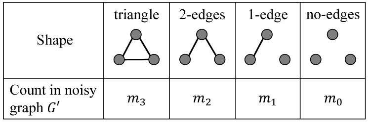
Through clever post-processing known as empirical estimation [31, 39, 57], we are able to obtain an unbiased estimate of $f_{\triangle}(G)$ from $G^{\prime}$. Specifically, a subgraph with three nodes can be divided into four types depending on the number of edges. Three nodes with three edges form a triangle. We refer to three nodes with two edges, one edge, and no edges as 2-edges, 1-edge, and no-edges, respectively. Figure 2 shows their shapes. $f_{\triangle}(G)$ can be expressed using $m_{3}$, $m_{2}$, $m_{1}$, and $m_{0}$ as follows:

Therefore, the data collector can count $m_{3}$, $m_{2}$, $m_{1}$, and $m_{0}$ from $G^{\prime}$, and calculate an unbiased estimate of $f_{\triangle}(G)$ by (4). In Appendix A, we show that the $l_{2}$ loss is significantly reduced by this empirical estimation.

Algorithm 2 shows this algorithm. In line 2, user $v_{i}$ applies the RR with privacy budget $\varepsilon$ (denoted by $RR_{\varepsilon}$) to $a_{i,1},\ldots,a_{i,i-1}$ in her neighbor list $\mathbf{a}_{i}$, and outputs $R_{i}=(RR_{\varepsilon}(a_{i,1}),\ldots,RR_{\varepsilon}(a_{i,i-1}))$. In other words, we apply the RR to the lower triangular part of $\mathbf{A}$ and there is no overlap between edges sent by users. In line 5, the data collector uses a function (denoted by UndirectedGraph) that converts the bits of $(R_{1},\ldots,R_{n})$ into an undirected graph $G^{\prime}=(V,E^{\prime})$ by adding edge $(v_{i},v_{j})$ with $i>j$ to $E^{\prime}$ if and only if the $j$-th bit of $R_{i}$ is $1$. Note that $G^{\prime}$ is biased, as explained above. In line 6, the data collector uses a function (denoted by Count) that calculates $m_{3}$, $m_{2}$, $m_{1}$, and $m_{0}$ from $G^{\prime}$. Finally, the data collector outputs the expression inside the expectation on the left-hand side of (4), which is an unbiased estimator for $f_{\triangle}(G)$ by Proposition 2. We denote this algorithm by LocalRR_△.

LocalRR_△ does not have the doubling issue (i.e., it provides not $2\varepsilon$ but $\varepsilon$-relationship DP), because we apply the RR to the lower triangular part of $\mathbf{A}$, as explained in Section 3.2.

Unlike the RR and empirical estimation for tabular data [31], the expected $l_{2}$ loss of LocalRR_△ is complicated. To simplify the utility analysis, we assume that $G$ is generated from the Erdös-Rényi graph distribution $\mathbf{G}(n,\alpha)$ with edge existence probability $\alpha$; i.e., each edge in $G$ with $n$ nodes is independently generated with probability $\alpha\in[0,1]$.

Note that we assume the Erdös-Rényi model only for the utility analysis of LocalRR_△, and do not assume this model for the other algorithms. The upper-bound of LocalRR_△ in Theorem 4 is less ideal than the upper-bounds of the other algorithms in that it does not consider all possible graphs $G\in\mathcal{G}$. Nevertheless, we also show that the $l_{2}$ loss of LocalRR_△ is roughly consistent with Theorem 4 in our experiments using two real datasets (Section 5) and the Barabási-Albert graphs [9], which have power-law degree distribution (Appendix B).

The parameters $\alpha$ and $\beta$ are edge existence probabilities in the original graph $G$ and noisy graph $G^{\prime}$, respectively. Although $\alpha$ is very small in a sparse graph, $\beta$ can be large for small $\varepsilon$. For example, if $\alpha\approx 0$ and $\varepsilon=1$, then $\beta\approx\frac{1}{e+1}=0.27$.

Theorem 4 states that for large $n$, the $l_{2}$ loss of LocalRR_△ ($=O(n^{4})$) is much larger than the $l_{2}$ loss of LocalRR${}_{k}\star$ ($=O(n)$). This follows from the fact that user $v_{i}$ is not aware of any triangle formed by $(v_{i},v_{j},v_{k})$, as explained above.

In contrast, counting $f_{\triangle}(G)$ in the centralized model is much easier because the data collector sees all triangles in $G$; i.e., the data collector knows $f_{\triangle}(G)$. The sensitivity of $f_{\triangle}$ is at most $\tilde{d}_{max}$ (after graph projection). Thus, we can consider a simple algorithm that outputs $f_{\triangle}(G)+\textrm{Lap}(\tilde{d}_{max}/\varepsilon)$. We denote this algorithm by CentralLap_△. CentralLap_△ attains the expected $l_{2}$ loss ($=$ variance) of $O\left(\frac{\tilde{d}_{max}^{2}}{\varepsilon^{2}}\right)$.

The large $l_{2}$ loss of LocalRR_△ is caused by the fact that each edge is released independently with some probability of being flipped. In other words, there are three independent random variables that influence any triangle in $G^{\prime}$. The next algorithm, using interaction, reduces this influencing number from three to one by using the fact that a user knows the existence of two edges for any triangle that involves the user.

As with the RR in Section 4.2, simply counting the noisy triangles can introduce a bias. Therefore, we calculate an empirical estimate of $f_{\triangle}(G)$ from the noisy triangle counts. Specifically, the following is the empirical estimate of $f_{\triangle}(G)$:

Note that in Proposition 3, we count only triplets $(v_{i},v_{j},v_{k})$ with $j<k<i$ to use only the lower triangular part of $\mathbf{A}$. $t_{i}$ is the number of noisy triangles user $v_{i}$ can see at the second round. $s_{i}$ is the number of $2$-stars of which user $v_{i}$ is a center. Since $t_{i}$ and $s_{i}$ can reveal information about an edge in $G$, user $v_{i}$ adds the Laplacian noise to $w_{i}$ $(=t_{i}-p_{1}s_{i})$ in (5), and sends it to the data collector. Then the data collector calculates an unbiased estimate of $f_{\triangle}(G)$ by (5).

References

- [1] Tool: LDP graph statistics. https://github.com/LDPGraphStatistics/LDPGraphStatistics.
- [2] 12th Annual Graph Drawing Contest. http://mozart.diei.unipg.it/gdcontest/contest2005/index.html, 2005.
- [3] What to Do When Your Facebook Profile is Maxed Out on Friends. https://authoritypublishing.com/social-media/what-to-do-when-your-facebook-profile-is-maxed-out-on-friends/, 2012.
- [4] AI bridging cloud infrastructure (ABCI). https://abci.ai/, 2020.
- [5] The diaspora* project. https://diasporafoundation.org/, 2020.
- [6] Facebook Reports Third Quarter 2020 Results. https://investor.fb.com/investor-news/press-release-details/2020/Facebook-Reports-Third-Quarter-2020-Results/default.aspx, 2020.
- [7] Jayadev Acharya, Clément L. Canonne, Yuhan Liu, Ziteng Sun, and Himanshu Tyagi. Interactive inference under information constraints. CoRR, 2007.10976, 2020.
- [8] Jayadev Acharya, Ziteng Sun, and Huanyu Zhang. Hadamard response: Estimating distributions privately, efficiently, and with little communication. In Proc. AISTATS’19, pages 1120–1129, 2019.
- [9] Albert-László Barabási. Network Science. Cambridge University Press, 2016.
- [10] Raef Bassily, Kobbi Nissim, Uri Stemmer, and Abhradeep Thakurta. Practical locally private heavy hitters. In Proc. NIPS’17, pages 2285––2293, 2017.
- [11] Raef Bassily and Adam Smith. Local, private, efficient protocols for succinct histograms. In Proc. STOC’15, pages 127–135, 2015.
- [12] Vincent Bindschaedler and Reza Shokri. Synthesizing plausible privacy-preserving location traces. In Proc. S&P’16, pages 546–563, 2016.
- [13] Jeremiah Blocki, Avrim Blum, Anupam Datta, and Or Sheffet. The johnson-lindenstrauss transform itself preserves differential privacy. In Proc. FOCS’12, pages 410–419, 2012.
- [14] Rui Chen, Gergely Acs, and Claude Castelluccia. Differentially private sequential data publication via variable-length n-grams. In Proc. CCS’12, pages 638–649, 2012.
- [15] Xihui Chen, Sjouke Mauw, and Yunior Ramírez-Cruz. Publishing community-preserving attributed social graphs with a differential privacy guarantee. Proceedings on Privacy Enhancing Technologies (PoPETs), (4):131–152, 2020.
- [16] Wei-Yen Day, Ninghui Li, and Min Lyu. Publishing graph degree distribution with node differential privacy. In Proc. SIGMOD’16, pages 123–138, 2016.
- [17] Bolin Ding, Janardhan Kulkarni, and Sergey Yekhanin. Collecting telemetry data privately. In Proc. NIPS’17, pages 3574–3583, 2017.
- [18] John Duchi and Ryan Rogers. Lower Bounds for Locally Private Estimation via Communication Complexity. arXiv:1902.00582 [math, stat], May 2019. arXiv: 1902.00582.
- [19] John Duchi, Martin Wainwright, and Michael Jordan. Minimax Optimal Procedures for Locally Private Estimation. arXiv:1604.02390 [cs, math, stat], November 2017. arXiv: 1604.02390.
- [20] John C. Duchi, Michael I. Jordan, and Martin J. Wainwright. Local privacy and statistical minimax rates. In Proc. FOCS’13, pages 429–438, 2013.
- [21] John C. Duchi, Michael I. Jordan, and Martin J. Wainwright. Local privacy, data processing inequalities, and minimax rates. CoRR, 1302.3203, 2014.
- [22] Cynthia Dwork. Differential privacy. In Proc. ICALP’06, pages 1–12, 2006.
- [23] Cynthia Dwork and Aaron Roth. The Algorithmic Foundations of Differential Privacy. Now Publishers, 2014.
- [24] Giulia Fanti, Vasyl Pihur, and Ulfar Erlingsson. Building a RAPPOR with the unknown: Privacy-preserving learning of associations and data dictionaries. Proceedings on Privacy Enhancing Technologies (PoPETs), 2016(3):1–21, 2016.
- [25] Ghurumuruhan Ganesan. Existence of connected regular and nearly regular graphs. CoRR, 1801.08345, 2018.
- [26] Aric A. Hagberg, Daniel A. Schult, and Pieter J. Swart. Exploring network structure, dynamics, and function using networkx. In Proceedings of the 7th Python in Science Conference (SciPy’08), pages 11–15, 2008.
- [27] Michael Hay, Chao Li, Gerome Miklau, and David Jensen. Accurate estimation of the degree distribution of private networks. In Proc. ICDM’09, pages 169–178, 2009.
- [28] Matthew Joseph, Janardhan Kulkarni, Jieming Mao, and Zhiwei Steven Wu. Locally Private Gaussian Estimation. arXiv:1811.08382 [cs, stat], October 2019. arXiv: 1811.08382.
- [29] Matthew Joseph, Jieming Mao, Seth Neel, and Aaron Roth. The Role of Interactivity in Local Differential Privacy. arXiv:1904.03564 [cs, stat], November 2019. arXiv: 1904.03564.
- [30] Matthew Joseph, Jieming Mao, and Aaron Roth. Exponential separations in local differential privacy. In Proc. SODA’20, pages 515–527, 2020.
- [31] Peter Kairouz, Keith Bonawitz, and Daniel Ramage. Discrete distribution estimation under local privacy. In Proc. ICML’16, pages 2436–2444, 2016.
- [32] Peter Kairouz, Sewoong Oh, and Pramod Viswanath. Extremal mechanisms for local differential privacy. Journal of Machine Learning Research, 17(1):492–542, 2016.
- [33] Vishesh Karwa, Sofya Raskhodnikova, Adam Smith, and Grigory Yaroslavtsev. Private analysis of graph structure. Proceedings of the VLDB Endowment, 4(11):1146–1157, 2011.
- [34] Shiva Prasad Kasiviswanathan, Homin K. Lee, Kobbi Nissim, and Sofya Raskhodnikova. What can we learn privately? In Proc. FOCS’08, pages 531–540, 2008.
- [35] Shiva Prasad Kasiviswanathan, Kobbi Nissim, Sofya Raskhodnikova, and Adam Smith. Analyzing graphs with node differential privacy. In Proc. TCC’13, pages 457–476, 2013.
- [36] Jure Leskovec and Andrej Krevl. SNAP Datasets: Stanford large network dataset collection. http://snap.stanford.edu/data, 2014.
- [37] Ninghui Li, Min Lyu, and Dong Su. Differential Privacy: From Theory to Practice. Morgan & Claypool Publishers, 2016.
- [38] Chris Morris. Hackers had a banner year in 2019. https://fortune.com/2020/01/28/2019-data-breach-increases-hackers/, 2020.
- [39] Takao Murakami and Yusuke Kawamoto. Utility-optimized local differential privacy mechanisms for distribution estimation. In Proc. USENIX Security’19, pages 1877–1894, 2019.
- [40] Kevin P. Murphy. Machine Learning: A Probabilistic Perspective. The MIT Press, 2012.
- [41] M. E. J. Newman. Random graphs with clustering. Physical Review Letters, 103(5):058701, 2009.
- [42] Kobbi Nissim, Sofya Raskhodnikova, and Adam Smith. Smooth sensitivity and sampling in private data analysis. In Proc. STOC’07, pages 75–84, 2007.
- [43] Thomas Paul, Antonino Famulari, and Thorsten Strufe. A survey on decentralized online social networks. Computer Networks, 75:437–452, 2014.
- [44] Venkatadheeraj Pichapati, Ananda Theertha Suresh, Felix X. Yu, Sashank J. Reddi, and Sanjiv Kumar. AdaCliP: Adaptive clipping for private SGD. CoRR, 1908.07643, 2019.
- [45] Zhan Qin, Yin Yang, Ting Yu, Issa Khalil, Xiaokui Xiao, and Kui Ren. Heavy hitter estimation over set-valued data with local differential privacy. In Proc. CCS’16, pages 192–203, 2016.
- [46] Zhan Qin, Ting Yu, Yin Yang, Issa Khalil, Xiaokui Xiao, and Kui Ren. Generating synthetic decentralized social graphs with local differential privacy. In Proc. CCS’17, pages 425–438, 2017.
- [47] Cyrus Rashtchian, David P. Woodruff, and Hanlin Zhu. Vector-matrix-vector queries for solving linear algebra, statistics, and graph problems. CoRR, 2006.14015, 2020.
- [48] Sofya Raskhodnikova and Adam Smith. Efficient lipschitz extensions for high-dimensional graph statistics and node private degree distributions. CoRR, 1504.07912, 2015.
- [49] Sofya Raskhodnikova and Adam Smith. Differentially Private Analysis of Graphs, pages 543–547. Springer, 2016.
- [50] Andrea De Salve, Paolo Mori, and Laura Ricci. A survey on privacy in decentralized online social networks. Computer Science Review, 27:154–176, 2018.
- [51] Tara Seals. Data breaches increase 40% in 2016. https://www.infosecurity-magazine.com/news/data-breaches-increase-40-in-2016/, 2017.
- [52] Shuang Song, Susan Little, Sanjay Mehta, Staal Vinterboy, and Kamalika Chaudhuri. Differentially private continual release of graph statistics. CoRR, 1809.02575, 2018.
- [53] Haipei Sun, Xiaokui Xiao, Issa Khalil, Yin Yang, Zhan Qui, Hui (Wendy) Wang, and Ting Yu. Analyzing subgraph statistics from extended local views with decentralized differential privacy. In Proc. CCS’19, pages 703–717, 2019.
- [54] Om Thakkar, Galen Andrew, and H. Brendan McMahan. Differentially private learning with adaptive clipping. CoRR, 1905.03871, 2019.
- [55] Abhradeep Guha Thakurta, Andrew H. Vyrros, Umesh S. Vaishampayan, Gaurav Kapoor, Julien Freudiger, Vivek Rangarajan Sridhar, and Doug Davidson. Learning New Words, US Patent 9,594,741, Mar. 14 2017.
- [56] Úlfar Erlingsson, Vasyl Pihur, and Aleksandra Korolova. RAPPOR: Randomized aggregatable privacy-preserving ordinal response. In Proc. CCS’14, pages 1054–1067, 2014.
- [57] Tianhao Wang, Jeremiah Blocki, Ninghui Li, and Somesh Jha. Locally differentially private protocols for frequency estimation. In Proc. USENIX Security’17, pages 729–745, 2017.
- [58] Yue Wang and Xintao Wu. Preserving differential privacy in degree-correlation based graph generation. Transactions on Data Privacy, 6(2), 2013.
- [59] Yue Wang, Xintao Wu, and Leting Wu. Differential privacy preserving spectral graph analysis. In Proc. PAKDD’13, pages 329–340, 2013.
- [60] Stanley L. Warner. Randomized response: A survey technique for eliminating evasive answer bias. Journal of the American Statistical Association, 60(309):63–69, 1965.
- [61] Xiaokui Xiao, Gabriel Bender, Michael Hay, and Johannes Gehrke. ireduct: Differential privacy with reduced relative errors. In Proc. SIGMOD’11, pages 229–240, 2011.
- [62] Min Ye and Alexander Barga. Optimal schemes for discrete distribution estimation under local differential privacy. In Proc. ISIT’17, pages 759––763, 2017.
- [63] Qingqing Ye, Haibo Hu, Man Ho Au, Xiaofeng Meng, and Xiaokui Xiao. Towards locally differentially private generic graph metric estimation. In Proc. ICDE’20, pages 1922–1925, 2020.
- [64] Qingqing Ye, Haibo Hu, Man Ho Au, Xiaofeng Meng, and Xiaokui Xiao. LF-GDPR: A framework for estimating graph metrics with local differential privacy. IEEE Transactions on Knowledge and Data Engineering (Early Access), pages 1–16, 2021.
- [65] Hailong Zhang, Sufian Latif, Raef Bassily, and Atanas Rountev. Differentially-private control-flow node coverage for software usage analysis. In Proc. USENIX Security’20, pages 1021–1038, 2020.
Appendix A Effectiveness of empirical estimation in LocalRR△
In Section 4.2, we presented LocalRR△, which uses the empirical estimation method after the RR. Here we show the effectiveness of empirical estimation by comparing LocalRR△ with the RR without empirical estimation [46, 63].
As the RR without empirical estimation, we applied the RR to the lower triangular part of the adjacency matrix ; i.e., we ran lines 1 to 6 in Algorithm 2. Then we output the number of noisy triangles . We denote this algorithm by RR w/o emp.
Figure 10 shows the loss of LocalRR△ and RR w/o emp when we changed from to or in edge LDP from to . The experimental set-up is the same as Section 5.1. Figure 10 shows that LocalRR△ significantly outperforms RR w/o emp, which means that the loss is significantly reduced by empirical estimation. As shown in Section 5, the loss of LocalRR△ is also significantly reduced by an additional round of interaction.
Appendix B Experiments on Barabási-Albert Graphs
Experimental set-up. In Section 5, we evaluated our algorithms using two real datasets: IMDB and Orkut. We also evaluated our algorithms using artificial graphs that have power-law degree distributions. We used the BA (Barabási-Albert) model [9] to generate such graphs.
In the BA model, an artificial graph (referred to as a BA graph) is grown by adding new nodes one at a time. Each new node is connected to existing nodes with probability proportional to the degree of the existing node. In our experiments, we used NetworkX [26], a Python package for graph analysis, to generate BA graphs.
We generated a BA graph with nodes using NetworkX. For the attachment parameter , we set or . When (resp. ), the average degree of was (resp. ). For each case, we randomly generated users from the whole graph , and extracted a graph with the users. Then we estimated the number of triangles and the number of -stars . For triangles, we evaluated LocalRR△, Local2Rounds△, and CentralLap. For -stars, we evaluated LocalLap and CentralLap. In Local2Rounds△, we set . For , we set .
We evaluated the loss while changing and . We attempted ways to randomly select users from , and averaged the loss over all the ways to randomly select users. As with Section 5, we set and changed from to while fixing . Then we set and changed from to while fixing .
Experimental results. Figure 11 shows the results. Overall, Figure 11 has a similar tendency to Figures 5, 6, and 7. For example, Local2Rounds△ significantly outperforms LocalRR△, especially when the graph is sparse; i.e., . In Local2Rounds△, CentralLap, LocalLap, and CentralLap, the loss increases with increase in . This is because the maximum degree increases with increase in .
Figure 11 also shows that the loss is roughly consistent with our upper-bounds in Section 4. For example, recall that LocalRR△, Local2Rounds△, CentralLap△, LocalLap2⋆, and CentralLap2⋆ achieve the expected loss of , , , , and , respectively. Assuming that , the left panels of Figure 11 are roughly consistent with these upper-bounds. In addition, the right panels of Figure 11 show that when we set and decrease from to , the loss increases by a factor of about , , and in LocalRR△, Local2Rounds△, and CentralLap△, respectively. They are roughly consistent with our upper-bounds – for small , the expected loss of LocalRR△, Local2Rounds△, and CentralLap△ is , , and , respectively.
In summary, for both the two real datasets and the BA graphs, our experimental results showed the following findings: (1) Local2Rounds△ significantly outperforms LocalRR△, especially when the graph is sparse; (2) our experimental results are roughly consistent with our upper-bounds.
Appendix C Construction of an independent cube for
Suppose that is even and is divisible by . Since , it is possible to write for integers such that and . Because and are even, we must have is even. Now, we can write . Thus, we can define a graph on nodes consisting of cliques of even size and one final clique of an even size with all cliques disjoint.
Since consists of even-sized cliques, it contains a perfect matching . Figure 12 shows examples of and , where , , , and . Let such that . Let . Each edge in is part of at least triangles. For each pair of edges in , the triangles of of which they are part are disjoint. Thus, for any edge , removing from a graph in will remove at least triangles. This implies that is an independent cube for .
Appendix D Proof of Statements in Section 4
Here we prove the statements in Section 4. Our proofs will repeatedly use the well-known bias-variance decomposition [40], which we briefly explain below. We denote the variance of the random variable by . If we are producing a private, randomized estimate of the graph function , then the expected loss (over the randomness in the algorithm) can be written as: