Localized Signaling Compartments in 2-D Coupled by a Bulk Diffusion Field: Quorum Sensing and Synchronous Oscillations in the Well-Mixed Limit

Sarafa A. Iyaniwura Michael J. Ward

Abstract

We analyze oscillatory instabilities for a coupled PDE-ODE system modeling the communication between localized spatially segregated dynamically active signaling compartments that are coupled through a passive extracellular bulk diffusion field in a bounded 2-D domain. Each signaling compartment is assumed to secrete a chemical into the extracellular medium (bulk region) and it can also sense the concentration of this chemical in the region around its boundary. This feedback from the bulk region, resulting from the entire collection of cells, in turn modifies the intracellular dynamics within each cell. In the limit where the signaling compartments are circular disks with a small common radius $\varepsilon\ll 1$ and where the bulk diffusivity is asymptotically large, a matched asymptotic analysis is used to reduce the dimensionless PDE-ODE system into a nonlinear ODE system with global coupling. For Sel’kov reaction kinetics, this ODE system for the intracellular dynamics and the spatial average of the bulk diffusion field is then used to investigate oscillatory instabilities in the dynamics of the cells that are triggered due to the global coupling. In particular, numerical bifurcation software on the ODEs is used to study the overall effect of coupling defective cells (cells that behave differently from the remaining cells) to a group of identical cells. Moreover, when the number of cells is large, the Kuramoto order parameter is computed to predict the degree of phase synchronization of the intracellular dynamics. Quorum sensing behavior, characterized by the onset of collective behavior in the intracellular dynamics as the number of cells increases above a threshold, is also studied. Our analysis shows that the cell population density plays a dual role of triggering and then quenching synchronous oscillations in the intracellular dynamics.

Key words: Hopf bifurcation, synchronous oscillations, quorum sensing, bulk diffusion, defector cells, Kuramoto order parameter, global coupling.

1 Introduction

Cell-cell communication is an important component of microbiological systems, which involves the sending and receiving of information from one cell to another. In a biological system consisting of unicellular organisms, cells coordinate and communicate with one another to accomplish tasks that cannot be achieved by a single cell. Those cells that are not in close proximity can only communicate through the extracellular space between them by both secreting and then sensing signaling chemicals in the extracellular medium, called autoinducers, and adjusting their intracellular activities accordingly. This bulk mediated form of cell-to-cell communication has been observed in many specific biological systems including, a collection of social amoebae Dictyostelium discoideum where the secretion of cyclic adenosine monophosphate (cAMP) by the cells triggers an oscillatory response and helps guide the cells to aggregation (cf. [10], [21]), colonies of yeast cells in which the exchange of acetaldehyde (Aca) molecules leads to glycolytic oscillations (cf. [4]), and the emergence of bioluminescence for the marine bacterium Vibrio fischeri at large cell densities (cf. [17]). In this context, the term quorum sensing refers to a process of cell-to-cell communication, mediated by a bulk diffusion field, that triggers some collective behavior of a group of cells as the cell density increases.

Quorum sensing phenomenon where the collective dynamics involves a switch-like emergence of synchronous oscillations as the cell density increases past a threshold has been observed and studied in several specific biological systems (cf. [4], [10], [12], [18], [14]) as well as in physicochemical systems involving small catalyst-loaded particles immersed in a chemical mixture (cf. [29], [28], [31], [30]). An overview of some universal features for quorum sensing systems in biology are discussed in [12]. In other cell signalling problems, spatio-temporal oscillations associated with chemically active, but spatially localized, sites that are mediated by a bulk diffusion field also arise in models of certain gene regulatory networks [2].

Refer to caption — Figure 1: A schematic diagram for (1.0.1) showing the dynamically active signaling compartments (in cyan) and the extracellular bulk region (unshaded) in a bounded 2-D domain. Each circular cell contains two signaling chemicals (red and green), but only the red chemical is secreted into the extracellular bulk region. A zoomed-in illustration of the secretion and feedback of chemicals into the cells is shown on the right.

Our goal herein is to use a theoretical framework based on a coupled PDE-ODE system to study the onset of synchronous intracellular dynamics in a collection of small signalling compartments or cells that are coupled through a 2-D passive bulk diffusion field. We begin by outlining the formulation of this coupled cell-bulk PDE-ODE model of [9], which was inspired by the models introduced in [19] (see also [20] and [32]). Let $\Omega\subset\mathbb{R}^{2}$ be a bounded domain that contains $m$ disk-shaped dynamically active signalling compartments or “cells” of a common radius $R$ , denoted by $\Omega_{j}$ and centered at $\boldsymbol{X}_{j}\in\Omega$ for $j=1,\dots,m$ . We assume that the concentration $\mathcal{U}(\boldsymbol{X},T)$ of the signaling molecule or autoinducer in the bulk or extracellular region $\Omega\setminus\cup_{j=1}^{m}\,\Omega_{j}$ , which is confined within $\partial\Omega$ , satisfies


	$\displaystyle\mathcal{U}_{T}=$	$\displaystyle D_{B}\,\Delta\,\mathcal{U}-k_{B}\,\mathcal{U}\,,\quad T>0\,,\quad\boldsymbol{X}\in\Omega\setminus\cup_{j=1}^{m}\,\Omega_{j}\,;$	(1.0.1a)
	$\displaystyle\,\partial_{n_{\boldsymbol{X}}}\,\mathcal{U}=0\,,\quad\boldsymbol{X}\in\partial\Omega\,,$	$\displaystyle\qquad D_{B}\,\partial_{n_{\boldsymbol{X}}}\,\mathcal{U}=\beta_{1,j}\,\mathcal{U}-\beta_{2,j}\,\mu_{j}^{1}\,,\qquad\boldsymbol{X}\in\partial\Omega_{j}\,,\quad j=1,2,\ldots,m\,.$	(1.0.1b)
Here $D_{B}>0$ and $k_{B}>0$ are the bulk diffusivity and the rate of degradation of the signaling chemical in the bulk region, respectively. In the Robin boundary condition (1.0.1b) on each cell boundary, $\beta_{1,j}>0$ and $\beta_{2,j}>0$ are dimensional constants modeling the permeability of the boundary for the $j^{\text{th}}$ cell, while $\partial_{n_{\boldsymbol{X}}}$ is the outward normal derivative pointing into the bulk region. Inside each dynamically active cell, which is assumed to be well-mixed, we suppose that there are $n$ interacting species, represented by the vector-field $\boldsymbol{\mu}_{j}\equiv(\mu_{j}^{1},\ldots,\mu_{j}^{n})^{T}$ , that if isolated from the bulk would interact according to the local reaction kinetics $\boldsymbol{F}_{j}\left(\boldsymbol{\mu}_{j}/\mu_{c}\right)$ . However, owing to the transport across each cell boundary, the bulk diffusion field of (1.0.1) is coupled to the local kinetics within the $j^{\text{th}}$ cell by
	$\begin{split}\frac{d\boldsymbol{\mu}_{j}}{dT}&=k_{R}\,\mu_{c}\,\boldsymbol{F}_{j}\left(\boldsymbol{\mu}_{j}/\mu_{c}\right)+\boldsymbol{e}_{1}\int_{\partial\Omega_{j}}\,\left(\beta_{1,j}\,\mathcal{U}-\beta_{2,j}\,\mu_{j}^{1}\right)\,\text{d}S_{\boldsymbol{X}}\,,\qquad j=1,\ldots,m\,.\end{split}$		(1.0.1c)

Here $\boldsymbol{e}_{1}\equiv(1,0,\ldots,0)^{T}$ , $k_{R}>0$ is the typical reaction rate for the dimensionless local kinetics $\boldsymbol{F}_{j}$ , and $\mu_{c}>0$ is a typical scalar measure of $\boldsymbol{\mu}_{j}$ . In this model, each cell secretes only one signaling chemical, labeled by $\mu_{j}^{1}$ , across its boundary into the bulk medium, and this secretion is regulated by the efflux permeability parameter $\beta_{2,j}$ . However, each cell receives feedback across its boundary, as controlled by the influx permeability parameter $\beta_{1,j}$ , from the entire collection of cells as mediated by the bulk concentration field $\mathcal{U}(\boldsymbol{X},T)$ for $\boldsymbol{X}\in\partial\Omega_{j}$ . Figure 1 shows a schematic diagram to illustrate the cell-bulk coupling in (1.0.1) for the case where there are $n=2$ intracellular species.

The coupled PDE-ODE model (1.0.1), non-dimensionalized in §2.1 and Appendix A and written in dimensionless form below in (2.1.1), is analyzed in the limit of a small common cell radius when the bulk diffusivity is sufficiently large so that the bulk medium can be considered as “well-mixed”. In this limit, where the leading-order bulk concentration field is spatially homogeneous, a matched asymptotic expansion analysis is used in §2.2 to reduce the dimensionless coupled PDE-ODE system (2.1.1) into an $nm+1$ component nonlinear ODE system, with global coupling, which is given below in (2.2.18). A similar reduction, but only for the case of identical cells, was given in §5 of [9]. We remark that our asymptotic reduction, starting from a governing PDE-ODE coupled system, provides a systematic method for deriving limiting globally coupled ODE systems characterizing cell-cell communication through a well-mixed bulk medium. This is in contrast to the more phenemologically-based ODE models used in previous studies (cf. [4], [22], [25], [18], [7]). Our limiting ODE system is related to those used in [16] and [15] to model communication between nonlinear oscillators coupled indirectly through an external medium.

For the specific case of Sel’kov reaction kinetics [26], the ODE system (2.2.18) for the intracellular dynamics and the spatial average of the bulk diffusion field is then used as a conceptual model to investigate the emergence of oscillatory instabilities in the intracellular dynamics that are triggered due to the global coupling. In the absence of coupling to the bulk medium, the Sel’kov kinetic parameters are chosen so that each cell is a conditional oscillator, in that its dynamics has only a stable steady-state when uncoupled from the bulk. As a result, in our study the emergence of intracellular oscillations is inherently due to the cell-cell interaction, as mediated by the global coupling through the well-mixed bulk region. However, in qualitative agreement with experimental findings in [4] and [3] involving yeast cells that are typically non-oscillatory when isolated, the Sel’kov parameters are chosen relatively close to the threshold for the onset of limit-cycle oscillations for an isolated cell.

With Sel’kov reaction kinetics, in §3 we compute global branches of steady-states and periodic solutions for the ODEs (2.2.18) using the numerical bifurcation software XPPAUT [6] for a small collection of cells. Our goal is to show how the permeability parameters, the Sel’kov kinetic parameters, and the number of cells influence the emergence of intracellular oscillations from a quiescent linearly stable steady-state. In our numerical bifurcation study in §3 we consider two main scenarios: one where all the cells are identical with common parameters, and the other a single defective cell, which has either different permeabilities or kinetic parameters, is coupled to a group of identical cells. Our numerical results, presented in the form of one- and two-parameter global bifurcation diagrams, show that for a collection of identical cells synchronous intracellular oscillations can occur in various parameter regimes as a result of the global coupling, even when their individual dynamics are linearly stable. Moreover, we show that small changes in the permeabilities or the reaction kinetics from a single defective cell can either extinguish or trigger intracellular oscillations of the entire group of cells. However, most typically, the range of these parameters that yields stable periodic solutions are smaller for the cases involving a defective cell, and this range decreases as the number of identical cells increases. Our theoretical finding that a single defective cell can trigger oscillations in the entire group is qualitatively similar to the observations in [10], based on live-cell imaging of the social bacteria Dictyostelium discoideum, that stochastic pulses originating from a discrete location play a critical role in the onset of collective oscillations. Our study of the effect of a defective cell on the entire group of cells is also related to game-theoretic concepts, which have recently been applied to quorum sensing behavior in microbial communities [1].

In §4 we recast the ODE system (2.2.18) in terms of a cell density parameter, defined by $\rho\equiv{m/|\Omega|}$ , in order to study the quorum sensing behavior associated with a large collection of either identical cells or a mixture of identical and defective cells. We show that the quorum sensing transition is characterized by the switch-like emergence of synchronous intracellular oscillations as $\rho$ crosses through a critical threshold. This is followed by a switch-like quenching of these oscillations as the cell density parameter crosses through a second, larger, threshold value. When the cells are identical, we show that these two threshold values are Hopf bifurcation points for a cubic polynomial. For a mixture of identical and defective cells, where a Sel’kov kinetic parameter is randomly chosen from some range, the quorum sensing and quenching thresholds are identified from a numerical computation of the Kuramoto order parameter, defined in (4.2.1) (see [15], [16]). The interval of the cell density parameter where the synchronization of intracellular dynamics occurs was found, as expected, to decrease as the number of defective cells increases.

In §5 we summarize some of our main results, and we discuss possible extensions of this study for investigating some specific biologically-based cell-cell communication problems that are mediated by a bulk diffusion field. Related problems that fit within the theoretical framework offered by the coupled PDE-ODE system (1.0.1) are also discussed.

2 The coupled PDE-ODE model: Non-dimensionalization and the well-mixed limit

In this section we non-dimensionalize the coupled PDE-ODE model (1.0.1) and study the dimensionless model in the large bulk diffusivity limit in a bounded 2-D domain. In this limit, the bulk region becomes well-mixed and the bulk concentration field becomes spatially homogeneous. In this well-mixed limit, a matched asymptotic analysis is used to reduce the dimensionless coupled PDE-ODE model into a system of ODEs with global coupling. This limiting system is used to investigate oscillatory instabilities in the intracellular dynamics and quorum sensing behavior.

2.1 Non-dimensionalization

We assume that the signaling compartments are circular with equal radius $R_{0}$ , which is small relative to the length-scale $L$ of the domain. As such, we introduce a small scaling parameter $\varepsilon\equiv R_{0}/L\ll 1$ . With this assumption, in Appendix A the coupled PDE-ODE model (1.0.1) is non-dimensionalized such that the dimensionless spatio-temporal bulk concentration field $U(\boldsymbol{x},t)$ satisfies


	$\displaystyle\tau\frac{\partial U}{\partial t}=$	$\displaystyle\,D\,\Delta U-\,U\,,\quad t>0\,,\quad\boldsymbol{x}\in\Omega\setminus\cup_{j=1}^{m}\,\Omega_{\varepsilon_{j}}\,;$	(2.1.1a)
	$\displaystyle\partial_{n}\,U=\,0,\quad\boldsymbol{x}\in\partial\Omega\,,$	$\displaystyle\qquad\varepsilon D\,\partial_{n_{j}}U=d_{1,j}\,U-d_{2,j}\,u_{j}^{1}\,,\quad\boldsymbol{x}\in\partial\Omega_{\varepsilon_{j}}\,,\quad j=1,\ldots,m\,,$	(2.1.1b)
where $\Omega_{\varepsilon_{j}}$ is a circular region of radius $\varepsilon\ll 1$ centered at $\boldsymbol{x}_{j}\in\Omega$ , representing the $j^{\text{th}}$ cell, $D$ is the effective diffusion coefficient in the bulk region, $\partial_{n}$ is the normal derivative pointing outward on the boundary of the domain $\Omega$ , and $\partial_{n_{j}}$ is the normal derivative on the boundary of the $j^{\text{th}}$ cell pointing out of the cell into the bulk medium. It is assumed that the cells are well-separated from each other in the sense that dist $(\boldsymbol{x}_{i},\boldsymbol{x}_{j})=\mathcal{O}(1)$ for $i\neq j$ , and that the center of each cell is at an $\mathcal{O}(1)$ distance from the boundary of the domain $\Omega$ , i.e. dist $(\boldsymbol{x}_{j},\partial\Omega)=\mathcal{O}(1)$ for $j=1,\dots,m$ as $\varepsilon\to 0$ . The dimensionless bulk concentration $U(\boldsymbol{x},t)$ is coupled to the local kinetics within the $j^{\text{th}}$ cell by
	$\begin{split}\frac{d\boldsymbol{u}_{j}}{dt}&=\,\boldsymbol{F}_{j}\left(\boldsymbol{u}_{j}\right)+\frac{\boldsymbol{e}_{1}}{\varepsilon\tau}\int_{\partial\Omega_{\varepsilon_{j}}}\,(d_{1,j}\,U-d_{2,j}\,u_{j}^{1})\,\,\text{d}s\,,\quad j=1,\ldots,m\,,\end{split}$		(2.1.1c)

where $\boldsymbol{u}_{j}\equiv(u_{j}^{1},\dots,u_{j}^{n})^{T}$ is a dimensionless vector representing the $n$ chemical species in the $j^{\text{th}}$ cell, $\boldsymbol{e}_{1}\equiv(1,0,\dots,0)^{T}$ , while $d_{1,j}>0$ and $d_{2,j}>0$ are dimensionless permeability parameters modelling the influx and efflux on the $j^{\text{th}}$ cell boundary, respectively. The intracellular, or local, kinetics within the $j^{\text{th}}$ cell is specified by the vector-field $\boldsymbol{F}_{j}\left(\boldsymbol{u}_{j}\right)$ . In (2.1.1), the dimensionless parameters are defined in terms of the parameters of (1.0.1) by

\begin{split}\tau\equiv\frac{k_{R}}{k_{B}}\,,\qquad D\equiv\frac{D_{B}}{k_{B}L^{2}}\,,\qquad d_{1,j}\equiv\frac{\varepsilon\beta_{1,j}}{k_{B}L}\,,\qquad d_{2,j}\equiv\frac{\varepsilon\beta_{2,j}L}{k_{B}}\,.\end{split}

(2.1.2)

With this non-dimensionalization, $\tau$ is large if the intracellular reactions occur quickly with respect to the time it takes the autoinducer signal to decay in the bulk medium. The dimensionless permeabilities $d_{1,j}$ and $d_{2,j}$ are taken to be $\mathcal{O}(1)$ , which implies that $\beta_{1,j}$ and $\beta_{2,j}$ are $\mathcal{O}(\varepsilon^{-1})$ since the length-scale $L$ of the domain and the rate $k_{B}$ of chemical decay in the bulk region are $\mathcal{O}(1)$ . In our analysis below, this scaling of the permeabilities is necessary in order to have significant secretion and feedback of chemicals into each signaling compartment in the limit $\varepsilon\to 0$ .

2.2 Asymptotic analysis in the well-mixed limit

In this subsection, we study the dimensionless coupled PDE-ODE model (2.1.1) in the well-mixed limit $D\gg\mathcal{O}(\nu^{-1})\gg\mathcal{O}(1)$ , where $\nu\equiv-1/\log\varepsilon$ . In this limit, the method of matched asymptotic expansions is used to reduce the coupled model (2.1.1) into a system of ODEs with global coupling.

For $D\gg\mathcal{O}(\nu^{-1})$ , we expand $U(\boldsymbol{x},t)$ in the (outer) bulk region at ${\mathcal{O}}(1)$ distances from the cells as

\begin{split}U(\boldsymbol{x},t)=U_{0}(\boldsymbol{x},t)+\frac{1}{D}\,U_{1}(\boldsymbol{x},t)+\cdots\end{split}

(2.2.1)

Upon substituting (2.2.1) into (2.1.1), and collecting terms in powers of $D$ , we obtain the leading-order problem

\begin{split}\Delta U_{0}=0\,,\quad&\boldsymbol{x}\in\Omega\setminus\{\boldsymbol{x}_{1},\ldots,\boldsymbol{x}_{m}\}\,;\qquad\partial_{n}U_{0}=0,\quad\boldsymbol{x}\in\partial\Omega\,,\end{split}

(2.2.2)

which has the solution $U_{0}\equiv U_{0}(t)$ . The next order problem for $U_{1}$ in the outer bulk region is

\begin{split}\Delta U_{1}=U_{0}+\tau U_{0t}\,,\quad&\boldsymbol{x}\in\Omega\setminus\{\boldsymbol{x}_{1},\ldots,\boldsymbol{x}_{m}\}\,;\qquad\partial_{n}U_{1}=0\,,\quad\boldsymbol{x}\in\partial\Omega\,,\end{split}

(2.2.3)

which must be supplemented by singularity conditions for $U_{1}$ as $\boldsymbol{x}\to\boldsymbol{x}_{j}$ , for each $j=1,\ldots,m$ .

To determine these conditions, we consider the inner region defined within an $\mathcal{O}(\varepsilon)$ neighborhood of the $j^{\text{th}}$ cell. In this region, we introduce the inner variables $\boldsymbol{y}=\varepsilon^{-1}(\boldsymbol{x}-\boldsymbol{x}_{j})$ and $U(\boldsymbol{x},t)=\mathcal{U}(\boldsymbol{x}_{j}+\varepsilon\boldsymbol{y},t)$ , with $\rho=|\boldsymbol{y}|$ . Upon writing (2.1.1a) and (2.1.1b) in terms of the inner variables, we obtain

\displaystyle\tau\,\mathcal{U}_{t}

\displaystyle=\frac{D}{\varepsilon^{2}}\,\Delta_{\boldsymbol{y}}\,\mathcal{U}-\,\mathcal{U}\,,\quad 1<\rho<\infty\,;\qquad D\,\partial_{\rho}\,\mathcal{U}=d_{1,j}\,\mathcal{U}-d_{2,j}\,u_{j}^{1}\,,\,\,\,\text{on}\,\,\,\rho=1\,,\qquad j=1,\ldots,m\,.

(2.2.4)

Since $D\gg\mathcal{O}(1)$ , we expand the inner solution $\mathcal{U}(\rho,t)$ in powers of $D$ as

\begin{split}\mathcal{U}(\rho,t)=\mathcal{U}_{0}(\rho,t)+\frac{1}{D}\,\mathcal{U}_{1}(\rho,t)+\cdots\,.\end{split}

(2.2.5)

Upon substituting (2.2.5) into (2.2.4), and collecting terms in powers of $D$ , we derive the leading-order inner problem

\begin{split}\Delta_{\rho}\,\mathcal{U}_{0}\equiv\frac{1}{\rho}\frac{\partial}{\partial\rho}\left(\rho\frac{\partial{\mathcal{U}}_{0}}{\partial\rho}\right)=0\,,&\quad 1<\rho<\infty\,;\qquad\partial_{\rho}\,\mathcal{U}_{0}=0\,,\quad\text{on}\quad\rho=1\,,\end{split}

(2.2.6)

near the $j^{\text{th}}$ cell. The solution to this problem which matches the outer solution as $\rho\to\infty$ is simply $\mathcal{U}_{0}\equiv U_{0}(t)$ .

We proceed to consider the next order problem in the inner region given by

\begin{split}\Delta_{\rho}\,\mathcal{U}_{1}&=0\,,\quad 1<\rho<\infty\,;\qquad D\,\partial_{\rho}\,\mathcal{U}_{1}=\,d_{1,j}\,\mathcal{U}_{0}-d_{2,j}\,u_{j}^{1}\,,\quad\text{on}\quad\rho=1\,,\qquad j=1,\ldots,m\,.\end{split}

(2.2.7)

Allowing logarithmic growth as $\rho\to\infty$ , the radially symmetric solution to this problem is

\begin{split}\mathcal{U}_{1,j}=(d_{1,j}\,\mathcal{U}_{0}-d_{2,j}\,u_{j}^{1})\log\rho+c_{j}\,,\qquad j=1,\ldots,m\,,\end{split}

(2.2.8)

where $c_{j}$ for $j=1,\ldots,m$ are unknown constants to be determined. We write this solution in terms of the outer variables and substitute the resulting expression into the inner expansion (2.2.5). For $\rho\to\infty$ , this yields that

\begin{split}\mathcal{U}\sim U_{0}+\frac{1}{D}\left[(d_{1,j}\,U_{0}-d_{2,j}u_{j}^{1})\,\log|\boldsymbol{x}-\boldsymbol{x}_{j}|+\frac{1}{\nu}(d_{1,j}\,U_{0}-d_{2,j}u_{j}^{1})\,+c_{j}\right]+\cdots,\quad j=1,\ldots,m\,.\end{split}

(2.2.9)

Since $D\gg\mathcal{O}(\nu^{-1})$ , where $\nu={-1/\log\varepsilon}$ , we have $1/{D\nu}\ll 1$ , which implies that $U_{0}$ is the largest term in the far-field behavior (2.2.9) of the inner solution. This estimate establishes the range of $D$ for which our analysis is valid. Upon matching the far-field behaviour of the inner solution given in (2.2.9) to the outer solution, we obtain the singularity behaviour of the outer solution $U_{1}$ as $\boldsymbol{x}\to\boldsymbol{x}_{j}$ . In this way, the complete outer problem for $U_{1}$ is given by


$\displaystyle\Delta U_{1}$	$\displaystyle=U_{0}+\tau U_{0t}\,,\quad\boldsymbol{x}\in\Omega\setminus\{\boldsymbol{x}_{1},\dots,\boldsymbol{x}_{m}\}\,;\qquad\partial_{n}U_{1}=0\,,\quad\boldsymbol{x}\in\partial\Omega\,;$	(2.2.10a)
$\displaystyle\vspace{0.5cm}U_{1}$	$\displaystyle\sim(d_{1,j}\,U_{0}-d_{2,j}\,u_{j}^{1})\,\log\|\boldsymbol{x}-\boldsymbol{x}_{j}\|\,,\quad\text{as}\quad\boldsymbol{x}\to\boldsymbol{x}_{j}\,,\quad j=1,\ldots,m\,.$	(2.2.10b)

By representing the singularity behaviour for $U_{1}$ given in (2.2.10b) in terms of a delta function for the PDE (2.2.10a), the problem for $U_{1}$ is equivalently written as

\begin{split}\Delta U_{1}&=(\tau U_{0t}+U_{0})+2\pi\sum_{j=1}^{m}(d_{1,j}\,U_{0}-d_{2,j}\,u_{j}^{1})\,\delta(\boldsymbol{x}-\boldsymbol{x}_{j})\,,\quad\boldsymbol{x}\in\Omega\,;\qquad\partial_{n}U_{1}=0\,,\quad\boldsymbol{x}\in\partial\Omega\,.\end{split}

(2.2.11)

Upon integrating (2.2.11) over the domain $\Omega$ and then applying the divergence theorem, we obtain

\begin{split}U_{0}^{\prime}=-\frac{1}{\tau}U_{0}-\frac{2\pi}{\tau|\Omega|}\sum_{j=1}^{m}(d_{1,j}\,U_{0}-d_{2,j}u_{j}^{1})\,,\end{split}

(2.2.12)

where $|\Omega|$ is the area of $\Omega$ . The chemical concentration in the bulk region is described at leading-order by this ODE, where the first term on the right hand side of the equation represents the decay of chemical in the bulk region, and the summation averages the net flux of chemical through the boundaries of all the signaling compartments.

To represent the solution to (2.2.11) we introduce the unique Neumann Green’s function $G(\boldsymbol{x};\boldsymbol{x}_{j})$ , which satisfies


$\displaystyle\Delta G$	$\displaystyle=\frac{1}{\|\Omega\|}-\delta(\boldsymbol{x}-\boldsymbol{x}_{j})\,,\quad\boldsymbol{x}\in\Omega\,;\qquad\partial_{n}G=0\,,\quad\boldsymbol{x}\in\partial\Omega\,;$	(2.2.13a)
$\displaystyle G(\boldsymbol{x};\boldsymbol{x}_{j})\sim-$	$\displaystyle\frac{1}{2\pi}\log\|\boldsymbol{x}-\boldsymbol{x}_{j}\|+R_{j}\,,\quad\text{as}\quad\boldsymbol{x}\to\boldsymbol{x}_{j}\,,\quad\text{and}\quad\int_{\Omega}\,G\,\text{d}\boldsymbol{x}=0\,,$	(2.2.13b)

where $R_{j}\equiv R(\boldsymbol{x}_{j})$ is its regular part at $\boldsymbol{x}=\boldsymbol{x}_{j}$ for $j=1,\ldots,m$ . Without loss of generality, we impose $\int_{\Omega}U_{1}\,\text{d}\boldsymbol{x}=0$ , so that the spatial average of $U$ in the bulk region to order ${\mathcal{O}}(\nu)$ is simply $U_{0}$ . Then, the solution to (2.2.11) is

U_{1}=-2\pi\sum_{i=1}^{m}\,(d_{1,i}\,U_{0}-d_{2,i}u_{i}^{1})\,G(\boldsymbol{x};\boldsymbol{x}_{i})\,.

(2.2.14)

Upon substituting (2.2.14) into the outer expansion (2.2.1), we obtain the two-term asymptotic expansion

\begin{split}U\sim U_{0}-\frac{2\pi}{D}\sum_{i=1}^{m}\,(d_{1,i}\,U_{0}-d_{2,i}\,u_{i}^{1})\,G(\boldsymbol{x};\boldsymbol{x}_{i})+\cdots\,,\end{split}

(2.2.15)

for the outer solution in the bulk region. Then, we expand (2.2.14) as $\boldsymbol{x}\to\boldsymbol{x}_{j}$ and use the singularity behaviour of the Neumann Green’s function given in (2.2.13b) to determine the constants $c_{j}$ for $j=1,\ldots,m$ in (2.2.8). Upon matching the local behavior of (2.2.15) to (2.2.9), we obtain that

\begin{split}c_{j}=-\left(\frac{1}{\nu}+2\pi\,R_{j}\right)(d_{1,j}\,U_{0}-d_{2,j}u_{j}^{1})\,-2\pi\sum_{i\neq j}^{m}\,(d_{1,i}\,U_{0}-d_{2,i}u_{i}^{1})\,G(\boldsymbol{x}_{j},\boldsymbol{x}_{i})\,,\qquad j=1,\ldots,m\,.\end{split}

(2.2.16)

In this way, (2.2.9) and (2.2.16) provide a two-term asymptotic expansion of the inner solution $\mathcal{U}(\rho,t)$ , which is valid within an $\mathcal{O}(\varepsilon)$ neigbourhood of the $j^{\text{th}}$ cell. This inner solution is given by

\begin{split}\mathcal{U}=U_{0}+\frac{1}{D}\left[(d_{1,j}\,U_{0}-d_{2,j}u_{j}^{1})\,\log\rho+\frac{1}{\nu}(d_{1,j}\,U_{0}-d_{2}u_{j}^{1})\,+c_{j}\right]+\cdots\,,\qquad j=1,\ldots,m\,.\end{split}

(2.2.17)

Lastly, we substitute the leading-order inner solution $U_{0}(t)$ into (2.1.1c) and evaluate the integral over the boundary of the $j^{\text{th}}$ cell. This provides the global coupling of the intracellular dynamics to the bulk solution.

In summary, in the well-mixed limit $D\gg{\mathcal{O}}(\nu^{-1})$ , where $\nu\equiv{-1/\log\varepsilon}$ and $\varepsilon\ll 1$ , the coupled PDE-ODE model (2.1.1) reduces to the following $nm+1$ dimensional nonlinear ODE system where the intracellular dynamics for $\boldsymbol{u}_{j}$ are globally coupled through the spatially uniform bulk diffusion field $U_{0}(t)$ :

\frac{dU_{0}}{dt}=-\frac{U_{0}}{\tau}-\frac{2\pi}{\tau|\Omega|}\sum_{j=1}^{m}(d_{1,j}\,U_{0}-d_{2,j}u_{j}^{1})\,;\qquad\frac{d\boldsymbol{u}_{j}}{dt}=\,\boldsymbol{F}_{j}\left(\boldsymbol{u}_{j}\right)+\frac{2\pi\boldsymbol{e}_{1}}{\tau}\,(d_{1,j}\,U_{0}-d_{2,j}\,u_{j}^{1})\,,\quad j=1,\ldots,m\,.

(2.2.18)

Here $\boldsymbol{e}_{1}=(1,0,...,0)^{T}$ , $m$ is the total number of signaling compartments/cells, $|\Omega|$ is the area of $\Omega$ , $\boldsymbol{u}_{j}=(u_{j}^{1},\dots,u_{j}^{n})^{T}$ is an $n$ -dimensional vector whose entries are the $n$ chemical species in the $j^{\text{th}}$ cell, and $\boldsymbol{F}_{j}(\boldsymbol{u}_{j})$ is the vector-field describing the local reaction kinetics within the $j^{\text{th}}$ cell.

3 Global bifurcation diagrams

In this section, we compute global bifurcation diagrams for (2.2.18) using the numerical bifurcation software XPPAUT [6] for the case where the intracellular species interact according to Sel’kov reaction kinetics. Sel’kov kinetics provides a two-component system of ODEs, which was originally used to qualitatively model oscillations in the glycolytic pathway (cf. [26]). For convenience of notation, we write the intracellular variable as $\mathbf{u}=(v,w)^{T}$ , and the local Sel’kov reaction kinetics $\boldsymbol{F}(\mathbf{u})$ as $\boldsymbol{F}(v,w)=(F(v,w),G(v,w))^{T}$ , where

\begin{split}F(v,w)\equiv\alpha w+wv^{2}-v\,,\qquad G(v,w)\equiv\epsilon_{0}(\mu-(\alpha w+wv^{2}))\,.\end{split}

(3.0.1)

Here $\alpha>0$ , $\mu>0$ and $\epsilon_{0}>0$ are the Sel’kov reaction parameters. The steady-state for Sel’kov dynamics ${dv/dt}=F(v,w)$ and ${dw/dt}=G(v,w)$ is $v_{e}=\mu$ and $w_{e}={\mu/(\alpha+\mu^{2})}$ , while the trace and determinant of the Jacobian matrix $J_{e}$ for this steady-state is readily calculated as

\det(J_{e})=\epsilon_{0}(\alpha+\mu^{2})\,,\qquad\text{tr}(J_{e})=2w_{e}v_{e}-1-\det(J_{e})=\frac{2\mu^{2}}{\alpha+\mu^{2}}-1-\epsilon_{0}(\alpha+\mu^{2})\,.

(3.0.2)

Since $\det(J_{e})>0$ , we conclude for the Sel’kov reaction kinetics that a single isolated cell, decoupled from the bulk medium, has a steady-state that is linearly stable if and only if $\text{tr}(J_{e})<0$ . The Hopf bifurcation boundary in the $\alpha$ versus $\mu$ parameter plane, as obtained by setting $\text{tr}(J_{e})=0$ is given by

\alpha=-\mu^{2}-\frac{1}{2\epsilon_{0}}+\frac{\sqrt{1+8\epsilon_{0}\mu^{2}}}{2\epsilon_{0}}\,.

(3.0.3)

By constructing a trapping region and appealing to the Poincare-Bendixson theorem, it is well-known that when the steady-state is unstable there is a time-periodic solution, characterized by a limit cycle, for the isolated cell. In contrast, when the steady-state is linearly stable there are no time-periodic oscillations with Sel’kov kinetics.

In our study of the ODE system (2.2.18), the Sel’kov kinetic parameters are chosen so that the steady-state of the intracellular dynamics within each cell is linearly stable, and hence no intracellular oscillations occur, when there is no coupling to the bulk diffusion field. When $\epsilon_{0}=0.15$ , this corresponds to choosing a pair $(\mu,\alpha)$ not within the green-shaded region in Figure 2. Our goal is to investigate intracellular oscillations that are triggered as a result of the global coupling through the bulk medium. Our results below are presented in the form of one- and two-parameter global bifurcation diagrams computed from (2.2.18) using XPPAUT [6]. When the cells are all identical, the bifurcation parameters are common to all of them. However, for the cases involving a defective cell, the bifurcation parameter is that of the defective cell only, which is identified as the cell with index $j=1$ .

3.0.1 Instability triggered by the rate of influx and efflux of the bulk chemical

We begin by studying the effect of the permeability parameters $d_{1}$ and $d_{2}$ on the intracellular dynamics. Recall that $d_{1,j}$ is the rate of chemical feedback (influx) from the bulk into the $j^{\text{th}}$ cell, while $d_{2,j}$ is the rate of secretion of chemical (efflux) by the cell into the bulk region. Our goal below is to investigate synchronous oscillations in the cells that are triggered by these parameters. One particular focus is to study how the intracellular dynamics of a collection of identical cells is altered due to changes in either the efflux or influx rate of one specific cell. The numerical bifurcation diagrams shown below exhibit how the permeabilities of such a single “defective” cell can significantly alter the parameter region where collective intracellular oscillations of the entire group of cells can occur.

In Figures 3(a) and 3(b) global branches of steady-state and periodic solutions for (2.2.18) are shown as the permeability parameter $d_{1}$ for $m=3$ and $m=8$ identical cells, respectively, is varied. In contrast, in Figures 3(c) and 3(d) we plot similar bifurcation diagrams but for the case where a single defective cell, having a modified permeability parameter $d_{1,1}$ , is coupled to the remaining identical cells of Figures 3(a) and 3(b). In both sets of figures the parameters used are $\alpha=0.9$ , $\epsilon_{0}=0.15$ , $\mu=2$ , $\tau=0.5$ and $d_{2}=0.2$ . In Figures 3(c) and 3(d), $d_{1}=0.8$ is used for the identical cells. We observe from these figures that the range of $d_{1}$ for which periodic solutions occur for (2.2.18) is bounded for this parameter set. Since $d_{1}$ is the rate of chemical feedback into the cells, a small value of $d_{1}$ implies little feedback of the bulk chemical into the cells and, hence, a weak coupling between the cells. As a result, since each cell has a linearly stable steady-state and no time-periodic oscillations when uncoupled from the bulk, one would expect no synchronous oscillations when $d_{1}$ is too small. This intuition is confirmed in Figures 3(a)–3(b). Alternatively, when $d_{1}$ is large relative to $d_{2}$ (rate of secretion of chemical into the extracellular medium), the secreted chemical is almost immediately fed back into the cells, which leads to a lower chemical concentration in the bulk region. As a result, the coupling between the cells is again weak, and one would expect that the steady-state is linearly stable and that no intracellular oscillations occur. This intuition is again confirmed in Figures 3(a)–3(b). Later in our numerical study (see Figure 5 below), we use two-parameter bifurcation diagrams to show that some specific ratios of $d_{1}$ and $d_{2}$ are required in order to trigger oscillatory instabilities of the steady-state. For $m=3$ identical cells (see Figure 3(a)), the range of $d_{1}$ that yields synchronous oscillations is $0.7613\leq d_{1}\leq 2.241$ , while for $m=8$ (see Figure 3(b)) that range is $0.2517\leq d_{1}\leq 0.8403$ . This indicates that the range of $d_{1}$ for which stable periodic solutions occur shrinks as the number of cells increases, and as a result it becomes increasingly difficult to synchronize the dynamics of the cells using the permeability parameter $d_{1}$ when $d_{2}$ is fixed. Figure 3(c) shows the result for two identical cells coupled to a defective cell, with intracellular oscillations occurring for $0.6277\leq d_{1,1}\leq 1.134$ . In Figure 3(d), where seven identical cells are coupled to a defective cell, intracellular oscillations occur only when $0.639\leq d_{1,1}\leq 0.9248$ . Similar to the case of identical cells, the range of $d_{1,1}$ for which linearly stable periodic solutions exist is larger when $m=3$ as compared to when $m=8$ . Most importantly, however, Figures 3(c) and 3(d) clearly show how rather small changes in the influx rate of a single defective cell, relative to the common value of the group, can act as a switch that quenches, or extinguishes, intracellular oscillations for the entire collection of cells.

The global bifurcation diagrams where the permeability parameter $d_{2}$ (the efflux rate of secretion of chemicals into the bulk region by the cells) is the bifurcation parameter are shown in Figure 4. The other parameter values are the same as those in Figure 3. Similar to the results for $d_{1}$ in Figure 3, the range of $d_{2}$ for which stable periodic solutions occur is bounded above and below for all the scenarios considered. Linearly stable steady-state solutions exist for small values of $d_{2}$ because the cells do not secrete enough chemical required to trigger oscillations. On the other hand, when the rate of secretion of chemicals is large relative to the rate of feedback of chemicals into the cells, there is insufficient chemical concentration within the cells to trigger oscillations. For $m=3$ and $m=8$ identical cells, we find that linearly stable synchronous periodic solutions occur on the ranges $0.07624\leq d_{2}\leq 0.2283$ and $0.1908\leq d_{2}\leq 0.5229$ , respectively. However, unlike the results in Figures 3(a) and 3(b), the range of $d_{2}$ that predicts synchronous oscillations becomes larger as the number of identical cells increases. For the case involving a defective cell, when $m=3$ (two identical cells and one defective cell) the Hopf bifurcation points are $d_{2,1}=0.1471$ and $d_{2,1}=0.2402$ , while for $m=8$ (seven identical and one defective cell) the Hopf bifurcation points are $d_{2,1}=0.1743$ and $d_{2,1}=0.2407$ . Since the range of $d_{2,1}$ that predicts stable periodic solutions is smaller when $m=8$ relative to when $m=3$ , this shows that when there is a defector cell it is more difficult to achieve synchronous oscillations as the overall population of cells increases. Comparing the identical cells cases (Figures 4(a) and 4(b)) with the cases involving a defective cell (Figures 4(c) and 4(d)), we observe that the range of $d_{2}$ that predicts linearly stable periodic solutions is larger, as expected, when the cells are identical. This indicates that cell-cell communication is more difficult to achieve when a single cell is secreting chemical at a different rate as compared to the other cells. More specifically, we observe that intracellular oscillations of the group can be extinguished by a defective cell that reduces its efflux rate. From comparing the results in Figures 3 and 4, we notice that the range of $d_{1}$ that synchronizes the intracellular dynamics of the cells is larger than that of $d_{2}$ for all the cases considered. This shows, for this parameter set, that it is easier to trigger communication among the cells using the rate of chemical feedback or influx from the bulk into the cells, rather than the rate of secretion of chemicals into the bulk.

Next, we present two-parameter global bifurcation diagrams in terms of the permeability parameters $d_{1}$ and $d_{2}$ . Figures 5(a) and 5(b) are for $m=3$ and $m=8$ identical cells, respectively, while Figures 5(c) and 5(d) are for the cases involving a defective cell. The remaining parameters are the same as those used in Figures 3 and 4. In Figures 5(a)–5(d), stable periodic solutions are predicted in the green wedge-shaped regions, while linearly stable steady-state solutions occur in the unshaded regions. From Figure 5 the region of intracellular oscillations are bounded by two straight black lines, consisting of Hopf bifurcation values for the steady-state solution that correspond to the one-parameter bifurcation diagrams in Figures 3 and 4. In other words, the one-parameter bifurcation diagrams in Figures 3 and 4 represent to taking vertical and horizontal slices through the parameter plane shown in Figures 5, respectively. We observe that as the number of identical cells increases there is a larger region in the permeability parameter space that lead to linearly stable synchronous intracellular oscillations (see Figure 5(b)). Moreover, the permeability parameter space that yields oscillations is relatively larger when the cells are all identical (Figure 5(a) and 5(b)), as compared to when a single defective cell has permeability parameters that are different from those of the group (Figure 5(c) and 5(d)). However, this is not the case for the scenario involving a defective cell. For this case, as the number of remaining identical cells increases, it becomes increasingly difficult to trigger intracellular oscillations of the group through changes in the permeability parameters of a single defective cell (see Figures 5(c) and 5(d)).

In Figure 14 of Appendix B we show a gallery of time-dependent solutions to the ODE system (2.2.18) for permeability parameter values sampled from the bifurcation diagrams in Figures 3–5.

3.0.2 Instability triggered by local reaction kinetics of the cells

In the previous subsection, we studied how intracellular oscillations are triggered by modifying the rate of influx ( $d_{1}$ ) and efflux ( $d_{2}$ ) of signaling chemicals across the cell boundaries. In this subsection, we use the ODE system (2.2.18) to study intracellular oscillations that are triggered by changes in the parameters of the local reaction kinetics. More specifically, in (3.0.1), the Sel’kov parameters $\mu>0$ and $\alpha>0$ are used as bifurcation parameters, while $\epsilon_{0}=0.15$ is fixed. In the results below, the permeabilities were fixed at $d_{1,j}=0.8$ and $d_{2,j}=0.2$ for $j=1,\dots,m$ .

Figure 6 shows the stability of the steady-state solutions of the ODEs (2.2.18) as $\alpha>0$ is varied. We observe from this figure that there is only one Hopf bifurcation point, $\alpha_{c}$ for $\alpha>0$ . For any value of $\alpha\leq\alpha_{c}$ , the ODE system has linearly stable periodic solutions with increasing amplitude as $\alpha$ decreases. Linearly stable steady-state solutions exist for $\alpha>\alpha_{c}$ . Figures 6(a) and 6(b) are for $m=3$ and $m=8$ identical cells, respectively. The amplitudes of the predicted oscillations for $m=3$ and $m=8$ are roughly similar, and the Hopf bifurcation threshold for $m=3$ at $\alpha_{c}=0.9182$ is a little larger than for $m=8$ where $\alpha_{c}=0.9042$ . Observe from Figure 2 that for a single isolated cell, uncoupled from the bulk, a Hopf bifurcation occurs when $\alpha\approx 0.694$ as computed from (3.0.3). For the defective cell case (Figures 6(c) and 6(d)), when $m=3$ (two identical cells with $\alpha=0.9$ and a defective cell), the Hopf bifurcation occurs at $\alpha_{c}=0.9562$ , while $\alpha_{c}=0.9342$ when $m=8$ cells (seven identical cells with $\alpha=0.9$ and a defective cell). As expected, similar to the case of identical cells, the Hopf bifurcation value of $\alpha$ for the defective cell is smaller than, and therefore closer to the stability boundary shown in Figure 2 (see equation (3.0.3)), as the number of cells increases. Most importantly, since for $\alpha=0.9$ there would be intracellular oscillations in the identical cells when the defective cell is absent, we observe from Figures 6(c) and 6(d) that when there is a defective cell then an increase in its kinetic parameter $\alpha$ above $\alpha_{c}$ will extinguish the intracellular oscillations of the entire group of cells. In contrast, from Figures 7(a) and Figures 7(b) we observe that a defective cell can trigger collective oscillations in a group of identical cells when the kinetic parameter of the defective cell decreases below a threshold. In Figures 7(a) and Figures 7(b) we fix $\alpha=0.93$ so that that no oscillations are possible for this group of identical cells. However, by adding a defective cell, we observe that intracellular oscillations for the entire group are triggered when the kinetic parameter for the defector satisfies $\alpha<\alpha_{c}\approx 0.8953$ for $m=3$ and $\alpha<\alpha_{c}\approx 0.7404$ for $m=8$ . Since $\alpha_{c}>0.694$ , the defective cell is still a conditional oscillator, and it would have a linearly stable steady-state when uncoupled from the bulk.

The global bifurcation diagrams with respect to the Sel’kov parameter $\mu>0$ are shown in Figure 8. For an isolated cell, uncoupled from the bulk, a horizontal slice at a sufficiently small value of $\alpha$ through the instability region in Figure 2 shows that there are two Hopf bifurcation values of $\mu$ for an isolated cell. The results in Figure 8 show how this instability region of an isolated cell is modified due to coupling with the bulk and in the presence of a defective cell. Similar to the results shown above when $\alpha$ was the bifurcation parameter, the range of $\mu$ that yields synchronous oscillations shrinks as the number of identical cells increases (see Figures 8(a) and 8(b)). For $m=3$ identical cells, Hopf bifurcations occur at $\mu_{1}=1.946$ and $\mu_{2}=2.987$ , and when $m=8$ they are at $\mu_{1}=1.845$ and $\mu_{2}=2.05$ . For the case of two identical cells (with $\mu=2$ ) and a defective cell, the Hopf bifurcation points are $\mu_{1}=1.842$ and $\mu_{2}=3.312$ (Figure 8(c)). Figure 8(d) shows the result for $m=8$ (seven identical cells with $\mu=2$ and a defective cell), which has three Hopf bifurcation points. This result shows that linearly stable periodic solutions exist for $0<\mu<0.3164$ and for $1.396<\mu<2.26$ . By comparing the results in Figures 8(c) and 8(d) we notice that the range of $\mu$ that predicts linearly stable periodic solutions is smaller when $m=8$ than when $m=3$ , even though synchronous oscillations are predicted in two different intervals when $m=8$ . This agrees with our earlier observation that an increase in the population of identical cells makes synchronization more difficult when they are coupled to a defective cell.

In Figure 9, we present two-parameter bifurcation diagrams for the Sel’kov parameters $\alpha$ and $\mu$ . In this figure, the green-shaded region is where linearly stable periodic solutions occur, while the unshaded region predicts linearly stable steady-state solutions. The results in Figures 6 and 8 correspond to vertical and horizontal slices through the two-parameter plane in Figure 9. The black dashed curve in Figure 9(a-d) is the Hopf bifurcation boundary of a single isolated cell, uncoupled from the bulk, as given in (3.0.3). In each subfigure, for any pair $(\mu,\alpha)$ in a green-shaded region that lies above this dashed curve, we conclude that the cell-cell coupling from the bulk medium is the trigger for intracellular oscillations that would otherwise not occur when the cells are decoupled from the bulk. In contrast, and most notably for three cells, we observe from Figures 8(a) and 8(c) that there are narrow parameter regimes where the black dashed curve is above the green region. These thin regimes correspond to where an oscillatory instability of an isolated cell is quenched by cell-cell coupling through the bulk medium.

When the cells are all identical, we observe by comparing Figure 8(a) and Figure 8(b) that the region where synchronous oscillations occur for $m=3$ cells is slightly larger than that for $m=8$ cells. This feature is in contrast to our observation from Figures 5(a) and 5(b) when the permeabilities were used as bifurcation parameters, where the parameter region of intracellular oscillations get larger as the number of cells increases. For the defective cell case, the existence of an additional regime of periodic solutions, as observed in Figure 8(d), is apparent in Figure 9(d). This new regime predicts linearly stable periodic solutions for large values of $\alpha$ , provided that $\mu>0$ is small enough, which is not apparent in the one-parameter bifurcation diagram for $\alpha$ presented in Figure 6(d). We notice from the result in Figure 9(b) that synchronous oscillations are not predicted as $\mu$ approaches zero when the cells are all identical. This indicates that the stable periodic solutions observed in Figure 9(d) as $\mu\to 0$ are triggered by the existence of a defective cell.

In Figure 15 of Appendix B we show a gallery of time-dependent solutions to the ODE system (2.2.18) for different Sel’kov kinetic parameters $\alpha$ and $\mu$ sampled from the bifurcation diagrams in Figures 6, 8 and 9.

3.0.3 Instabilities due to increasing the number of cells

In this subsection, we determine how parameter regimes for linearly stable periodic solutions change as the number of cells increases. Our findings are presented as two-parameter Hopf bifurcation diagrams, where the vertical axis is one of our main bifurcation parameters and the horizontal axis is the number of cells, the latter of which is treated for convenience as a continuous rather than a discrete variable. In Figure 10 and Figure 11, linearly stable periodic solutions are predicted in the green-shaded regions, while linearly stable solutions are predicted in the unshaded regions. The parameter values are in the caption of these figures. Since synchronous oscillations occur as the cell population increases, these results can also be used to study quorum sensing behavior for a fixed value of each parameter. Starting with the case of identical cells, Figure 10(a) shows the result for the permeability parameter $d_{1}$ , which agrees with the result in Figure $18$ of [9]. It predicts that linearly stable periodic solutions can be triggered in the system for $m\leq 35$ . For each population size $m$ , and for fixed $d_{2}$ , there is a range of $d_{1}$ for which synchronous oscillations exist, and this range widens as the number of cells decreases. This trend is qualitatively different than that shown in Figure 10(b) with regards to $d_{2}$ at a fixed value of $d_{1}$ . For this permeability parameter, linearly stable periodic solutions exist for all values of $m$ in some finite interval of $d_{2}$ , and this range widens as the number of cells increases. Since $d_{2}$ is the efflux rate out of a cell, the observation that the Hopf bifurcation threshold for $d_{2}$ increases as $m$ increases, indicates that more signaling chemical is needed to synchronize the intraceulluar dynamics of a larger number of cells. Figure 10(c) shows the corresponding result for the Sel’kov parameter $\alpha>0$ . The black dashed horizontal line in this figure at $\alpha\approx 0.694$ is the Hopf bifurcation threshold of a single isolated cell when uncoupled from the bulk. We observe from this figure that linearly stable periodic solutions can occur for any number of cells, even when each cell has a linearly stable steady-state when uncoupled from the bulk. However, as seen in Figure 10(d), this is not the case for $\mu>0$ , where linearly stable synchronous solutions are predicted only for $m\leq 8$ on some range of $\mu$ that decreases as the number of cells increases. No oscillation is predicted for any value of $\mu$ when $m\geq 9$ .

Similar results, but predicting qualitatively different outcomes, are presented in Figure 11 for the case of a single defective cell coupled to a group of identical cells. In these results, the bifurcation parameters $d_{1}$ , $d_{2}$ , $\alpha$ and $\mu$ are for the defective cell only, and $m$ is the population of identical cells. From Figure 11(a), for $2\leq m\leq 7$ , there is a finite range of permeabilities $d_{1,1}$ for which intracellular oscillations can occur. On this range of $m$ , variations in $d_{1,1}$ can either trigger or extinguish intracellular oscillations. No oscillations can occur for $m\geq 8$ . From Figure 11(b) similar conclusions hold for the second permeability parameter $d_{2,1}$ . We observe from Figures 11(a) and 11(b) that variations in the cell population $m$ also play a dual role of triggering and quenching intracellular oscillations.

In Figure 11(c) we show that when the number of identical cells with a common Sel’kov parameter $\alpha=0.9$ satisfies $m\leq 18$ , intracellular oscillations for the group of cells can still occur when a defective cell is included, provided that the Sel’kov parameter for the defective cell is below some threshold. Without the defective cell, if there are more than seven identical cells with a common Sel’kov parameter $\alpha=0.9$ there are no oscillations, as $m\geq 7$ and $\alpha=0.9$ is not within the green-shaded region of Figure 10(c). However, on the range $10\leq m\leq 18$ , we observe from Figure 11(c) that to maintain intracellular oscillations the defective cell is no longer a conditional oscillator, as its required value of $\alpha$ is below the horizontal black dashed line in Figure 11(c). With regards to $\mu$ , Figure 11(d) shows the qualitatively different feature that there are two regimes of $\mu$ for which intracellular oscillations occur for different ranges of $m$ . As $m$ increases, there is initially only one regime in $\mu$ for which periodic solutions exists. However, as the cell population increases, a new regime emerges when $m=5$ . These two regimes co-exist until $m=8$ , after which the first regime vanishes, and the second one continues until $m=9$ . There are no intracellular oscillations in the system for $m>9$ .

4 Quorum sensing and phase synchronization: The Kuramoto order parameter

In this section, we use the ODE system (2.2.18) to study quorum sensing (QS) behavior, characterized by the emergence of collective cell dynamics that arises from a quiescent state as the cell population density exceeds a threshold. Since the ratio of the area occupied by $m$ circular cells of a common radius $\varepsilon$ to the overall domain area is ${m\pi\varepsilon^{2}/|\Omega|}$ , our measure of the cell density is taken as $\rho\equiv{m/|\Omega|}$ . With our Sel’kov kinetics, we will define collective dynamics as the emergence of synchronous oscillations in the intracellular dynamics as $\rho$ exceeds a critical value.

In terms of the parameter $\rho\equiv m/|\Omega|$ , the ODE system (2.2.18) becomes

\begin{split}\frac{dU_{0}}{dt}&=-\frac{1}{\tau}U_{0}-\frac{\rho}{m}\sum_{j=1}^{m}(k_{1,j}\,U_{0}-k_{2,j}u_{j}^{1})\,,\quad\frac{d\boldsymbol{u}_{j}}{dt}=\,\boldsymbol{F}_{j}\left(\boldsymbol{u}_{j}\right)+\boldsymbol{e}_{1}\,(k_{1,j}\,U-k_{2,j}\,u_{j}^{1})\,,\qquad j=1,\ldots,m\,,\end{split}

(4.0.1)

where we have defined $k_{1,j}\equiv(2\pi d_{1,j})/\tau$ and $k_{2,j}\equiv(2\pi d_{2,j})/\tau$ . For the case of identical cells, we will perform a Hopf bifurcation analysis on this system in order to identify the range of instability of the steady-state as $\rho$ is varied. For the case of non-identical cells, in §4.2 the Kuramoto order parameter (cf. [23], [16], [15]) will be used to measure the degree of phase synchrony of the intracellular oscillations.

4.1 Hopf bifurcation analysis for identical cells

For the case where the cells are all identical we label $k_{1}\equiv k_{1,j}$ and $k_{2}\equiv k_{2,j}$ , and introduce the common local variables $\boldsymbol{u}=\boldsymbol{u}_{j}$ and $\boldsymbol{F}(\boldsymbol{u})\equiv\boldsymbol{F}_{j}(\boldsymbol{u}_{j})$ for $j=1,\dots,m$ . For this identical cell case, (4.0.1) reduces to

\begin{split}\frac{dU_{0}}{dt}&=-\frac{1}{\tau}U_{0}-\rho\,(k_{1}\,U_{0}-k_{2}u^{1})\,,\qquad\frac{d\boldsymbol{u}}{dt}=\,\boldsymbol{F}\left(\boldsymbol{u}\right)+\boldsymbol{e}_{1}\,(k_{1}\,U-k_{2}\,u^{1})\,,\end{split}

(4.1.1)

where $U_{0}\equiv U_{0}(t)$ is the leading-order concentration of the signaling chemical in the bulk region and $\boldsymbol{u}=(u^{1},\ldots,u^{n})^{T}$ represents the $n$ interacting chemical species in the cells. Upon substituting the Sel’kov reaction kinetics (3.0.1) into (4.1.1), for which $n=2$ , we readily calculate that the steady-state solution $(U_{0e},u_{e}^{1},u_{e}^{2})$ is

\begin{split}U_{0e}=\frac{\tau\mu\rho k_{2}}{(1+k_{2}+\tau\rho k_{1})}\,,\quad u_{e}^{1}=\frac{\mu(1+\tau\rho k_{1})}{(1+k_{2}+\tau\rho k_{1})}\,,\quad u_{e}^{2}=\frac{\mu}{\left(\alpha+(u_{e}^{1})^{2}\right)}\,,\quad\text{where}\quad\boldsymbol{u}_{e}=(u_{e}^{1},u_{e}^{2})^{T}\,.\end{split}

(4.1.2)

From (4.1.2) we observe that both the steady-state bulk concentration $U_{0e}$ and $u_{e}^{1}$ are increasing functions of the cell density parameter $\rho$ . Moreover, as expected, $U_{0e}$ is an increasing function of the cell efflux rate $k_{2}$ , but decreases as the influx rate $k_{1}$ into the cells increases. As the influx rate $k_{1}$ into the cells from the bulk medium increases, the intracellular level $u_{e}^{1}$ also increases. In the large cell density limit we obtain from (4.1.2) that

u_{e}^{1}\to\mu\,,\qquad u_{e}^{2}\to\frac{\mu}{\alpha+\mu^{2}}\,,\qquad U_{0e}\to\frac{\mu k_{2}}{k_{1}}\,,\qquad\mbox{as}\quad\rho\to\infty\,.

(4.1.3)

These limiting values for the intracellular species are the same as those for a single cell that is uncoupled from the bulk medium, as summarized in §3.

To determine the linear stability of this steady-state, we introduce the perturbation

\begin{split}U&=U_{0e}+e^{\lambda t}\eta\,,\qquad\boldsymbol{u}=\boldsymbol{u}_{e}+e^{\lambda t}\boldsymbol{\phi}\,,\end{split}

(4.1.4)

where $|\boldsymbol{\phi}|\ll 1$ and $\eta\ll 1$ . Upon substituting (4.1.4) into (4.1.1), we obtain the linearized system

\begin{split}\lambda\eta&=-\frac{\eta}{\tau}-\rho(k_{1}\eta-k_{2}\phi_{1})\,,\qquad\lambda\boldsymbol{\phi}=J_{e}\boldsymbol{\phi}+\boldsymbol{e}_{1}(k_{1}\eta-k_{2}\phi_{1})\,,\end{split}

(4.1.5)

where $J_{e}$ is the Jacobian matrix of the local kinetics $\boldsymbol{F}(\boldsymbol{u})=(F(u^{1},u^{2}),G(u^{1},u^{2}))^{T}$ evaluated at the steady-state solution $\boldsymbol{u}_{e}=(u_{e}^{1},u_{e}^{2})^{T}$ , and $\boldsymbol{\phi}=(\phi_{1},\phi_{2})^{T}$ . For convenience of notation, we let $(v,w)\equiv(u_{e}^{1},u_{e}^{2})$ , and write the linearized system (4.1.5) in matrix form as

\begin{split}\mathcal{H}(\lambda)\boldsymbol{\Psi}=\boldsymbol{0}\,,\end{split}

(4.1.6)

where $\boldsymbol{\Psi}=(\eta,\phi_{1},\phi_{2})^{T}$ and $\mathcal{H}(\lambda)$ is the $3\times 3$ matrix defined by

\begin{split}\mathcal{H}(\lambda)=\begin{pmatrix}-\left(\frac{1}{\tau}+\rho k_{1}\right)-\lambda&\rho k_{2}&0\\ \\ k_{1}&(F_{v}^{e}-k_{2}-\lambda)&F_{w}^{e}\\ \\ 0&G_{v}^{e}&(G_{w}^{e}-\lambda)\end{pmatrix}\,.\end{split}

(4.1.7)

Here $F_{v}^{e},F_{w}^{e},G_{v}^{e}$ , and $G_{w}^{e}$ denote the partial derivatives of $F$ or $G$ with respect to $v$ or $w$ evaluated at the steady-state $\boldsymbol{u}_{e}$ . A simple calculation shows that there is a nontrivial solution to (4.1.6) if only if $\lambda$ is a root of the cubic

	$\begin{split}\lambda^{3}+p_{1}\lambda^{2}+p_{2}\lambda+p_{3}=0\,,\end{split}$	(4.1.8a)
whose coefficients are given by
	$\begin{split}p_{1}\equiv\left(k_{2}+\frac{1}{\tau}+\rho k_{1}\right)&-\text{tr}(J_{e})\,,\qquad p_{2}\equiv(1+k_{2})\det(J_{e})-\left(\frac{1}{\tau}+\rho k_{1}\right)\text{tr}(J_{e})+\frac{k_{2}}{\tau}\,,\\ p_{3}&\equiv\left(\frac{1}{\tau}+\rho k_{1}+\frac{k_{2}}{\tau}\right)\det(J_{e})\,.\end{split}$	(4.1.8b)

Here $\det(J_{e})=F_{v}^{e}G^{e}_{w}-F_{w}^{e}G^{e}_{v}>0$ and $\text{tr}(J_{e})=F_{v}^{e}+G_{w}^{e}$ are the determinant and trace of $J_{e}$ for Sel’kov reaction kinetics, for which we readily calculate that $\det(J_{e})=-G_{w}^{e}=\epsilon_{0}(\alpha+v_{e}^{2})$ . By the Routh-Hurwitz criterion for cubic functions, the three roots of the polynomial (4.1.8a) satisfy $\mbox{Re}(\lambda)<0$ if and only if the following conditions hold

\begin{split}p_{1}>0\,,\qquad p_{3}>0\,,\qquad\text{and}\quad p_{1}p_{2}>p_{3}\,.\end{split}

(4.1.9)

From (4.1.8b) we observe that $p_{3}>0$ always holds. Since we are interested in finding Hopf bifurcation points, we need to consider a special cubic polynomial whose roots satisfy $\lambda_{1}=a<0$ , $\lambda_{2,3}=\pm i\omega$ , for which

\begin{split}(\lambda-a)(\lambda-i\omega)(\lambda+i\omega)=\lambda^{3}-a\lambda^{2}+\omega^{2}\lambda-a\omega^{2}=0\,.\end{split}

(4.1.10)

Upon comparing the polynomials (4.1.8a) and (4.1.10), we conclude that a Hopf bifurcation threshold must satisfy

\begin{split}p_{1}>0\,,\quad p_{3}>0\,,\quad\text{and}\quad p_{1}p_{2}=p_{3}\,.\end{split}

(4.1.11)

For the parameter values in the caption of Figure 12, we use (4.1.11) to numerically compute two Hopf bifurcation points at $\rho_{1}=0.8010$ and $\rho_{2}=2.6750$ . These results agree with those computed in Figure 12 using XPPAUT [6].

Figure 12(a) shows a one-parameter Hopf bifurcation diagram for the ODE system (4.1.1) with respect to the cell population density $\rho$ parameter. Observe from this figure that the range of $\rho$ that predicts stable periodic solutions is bounded. This indicates that the cell population density plays a dual role of both triggering and then quenching intracellular oscillations, which agrees with our earlier observation in Figure 11. Our results in Figure 12(a) show that there are no synchronous oscillations for $\rho<0.8010$ and for $\rho>2.6750$ , and that linearly stable periodic solutions exist only on the range $0.8010\leq\rho\leq 2.6750$ . As $\rho$ increases above $\rho=0.8010$ , synchronous oscillations are triggered through quorum sensing behavior. These two Hopf bifurcation values for $\rho$ generate the green wedge-shaped region shown in Figure 12(b) in the $m$ versus $|\Omega|$ parameter plane where synchronous intracellular oscillations occur. For any vertical slice through the bifurcation diagram in Figure 12(b), corresponding to a domain of fixed area $|\Omega|$ , there is a quorum sensing threshold for the number of cells required to trigger synchronous oscillations. Moreover, there is an additional threshold on the number of cells for which the oscillations are quenched. This clearly shows that the cells adjust their intracellular dynamics in accordance with the number of cells in the population. When the domain area is small, fewer cells are required to trigger oscillations, while as the domain area increases the number of cells required for quorum sensing also increases. On the other hand, the quenching of oscillations predicted by Figure 12(b) results from having too many cells in a given domain area. As the domain area increases, the number of cells required to quench oscillations also increases, as expected intuitively. The qualitative mechanism underlying the quenching of oscillations is that when $\rho\gg 1$ the collection of cells behaves like a single “effective” cell, which has no intracellular oscillations and a unique linearly stable steady-state as result of the Sel’kov parameters chosen. Mathematically, as $\rho\to\infty$ , we have $v_{e}\to\mu$ and $w_{e}\sim{\mu/(\alpha+\mu^{2})}$ from (4.1.3), and so from (3.0.2) and the fact that the Sel’kov kinetic parameters were chosen so that a single isolated cell has a linearly steady-state, we must have $\text{tr}(J_{e})<0$ for $\rho\gg 1$ . Therefore, from (4.1.8b) we obtain that $p_{1}>0$ for $\rho$ sufficiently large. Moreover, since from (4.1.8b) we have

p_{1}p_{2}\sim\rho^{2}k_{1}^{2}|\text{tr}(J_{e})|={\mathcal{O}}(\rho^{2})\,,\qquad p_{3}\sim\rho k_{1}\left(\det{J_{e}}\right)={\mathcal{O}}(\rho)\,,\qquad\mbox{as}\quad\rho\to\infty\,,

(4.1.12)

we conclude that $p_{1}p_{2}>p_{3}$ for $\rho$ sufficiently large. Therefore, when $\rho$ is sufficiently large the Routh-Hurwitz conditions in (4.1.9) are satisfied. As a result, there must be a critical value $\rho_{m}$ of the cell density parameter $\rho$ , with $\rho_{m}$ sufficiently large, for which the steady-state of the ODE system (4.1.1) is linearly stable for all $\rho>\rho_{m}$ .

We emphasize that the two bifurcation diagrams in Figure 12 are related. A vertical slice of the one-parameter Hopf bifurcation diagram in Figure 12(a) at a population density of $\rho=\rho_{s}$ corresponds to a straight line with slope $\rho_{s}$ (since $\rho=m/|\Omega|$ ) passing through the origin in the two-parameter bifurcation diagram in Figure 12(b). The Hopf bifurcation points $\rho_{1}=0.8010$ and $\rho_{2}=2.6750$ in Figure 12(a) are the slopes of the Hopf bifurcation boundaries in Figure 12(b). Any straight line passing through the origin and contained between these boundaries corresponds to a vertical slice of the one-parameter bifurcation diagram in Figure 12(a) at a $\rho$ value between $\rho_{1}$ and $\rho_{2}$ .

4.2 Phase synchronization and the order parameter

Next, we study quorum sensing using the ODE system (4.0.1) together with the Kuramoto order parameter. The Kuramoto order parameter was originally used to measure the degree of phase synchrony of a system of coupled oscillators [13]. We will use the version of the order parameter presented in [15] and [16], given by

\displaystyle R=\left\langle\left|N^{-1}\sum_{j=1}^{N}\,\,\exp[i\theta_{j}(t)]-\left\langle N^{-1}\sum_{j=1}^{N}\,\,\exp[i\theta_{j}(t)]\right\rangle\right|\right\rangle\,,

(4.2.1)

which was used in [15] and [16] to measure the degree of phase synchrony of indirectly coupled chaotic oscillators. Here $N$ is the number of oscillators, $\theta_{j}(t)$ is the instantaneous phase of the $j^{\text{th}}$ oscillator, and $\langle\dots\rangle$ represents average over time. The value of $R$ indicates the level of phase synchronization of the oscillators, and it varies between 0 and 1, inclusive. When $R=1$ , the oscillators are perfectly in phase, while the value $R=0$ indicates that they are perfectly out of phase. Two oscillators are said to be in phase if their frequency and phase angles are the same at each cycle as they oscillate. Our goal is to use the system of ODEs (4.0.1) together with the order parameter (4.2.1) to measure the degree of phase synchronization of the intracellular dynamics within the signaling compartments as the population density $\rho$ is varied. In our numerical examples below, the cell population will be taken to be a mixture of identical and defective cells, where the heterogeneous cells have one different Sel’kov parameter.

To measure the degree of synchronization of the cells, we first solved the coupled system of ODEs (4.0.1) numerically using ODE45 in MATLAB [27]. The solution over the transient period was discarded, after which we extracted the time evolution of the same chemical species in all the cells. Only one of the intracellular chemical species was used for this analysis because both of them started oscillating and synchronizing at the same time. A single mode Fourier series expansion was fitted to each of the selected solutions, and their instantaneous phase $\theta(t)$ was computed from the coefficients of the series. At each time point, the phase of each oscillator was mapped to the complex number $e^{i\theta}$ (where $i=\sqrt{-1}$ ) on the unit circle, and an average of these points was computed using $z=N^{-1}\sum_{j=1}^{N}e^{i\theta_{j}}$ . For better intuition of the meaning of this average, take each point on the unit circle to be a unit vector. Then $z$ is a vector whose direction is the average direction of all the vectors on the unit circle. The length of this average vector is bounded between 0 and 1, which indicates the degree of phase synchrony of the oscillators at that time point. For instance, if two oscillators are perfectly synchronized at a specific time point, their phases at that point will be the same and they will both be mapped to the same point on the unit circle. The average of these two points/vectors gives another unit vector in the same direction. The fact that their average is a unit vector verifies that the two oscillators are in perfect synchrony at this point. On the other hand, if the two oscillators are completely out of phase, their phases will be mapped to opposite ends of the unit circle, and their average will be the zero vector, so that $|z|=0$ . The more synchronized oscillators are at a time point, the closer the corresponding mapping of their phases are on the unit circle, and as a result the closer the value of $|z|$ is to 1. Thus, $|z|$ indicates the level of synchrony of the oscillators at each time point. Upon computing the instantaneous averages at each time point, we computed their average over a specified time interval (after the system has reached a quasi steady-state). Lastly, the modulus of the difference between the instantaneous averages $z$ and the time-average $\langle z\rangle$ was computed for each time point, and then the corresponding result was averaged over time to calculate the order parameter $R$ , as given in (4.2.1) (cf. [16], [23]). In our computations below, we set $R=0$ when the cells are in a quiescent state and whenr oscillations have an amplitude less than $1\times 10^{-4}$ .

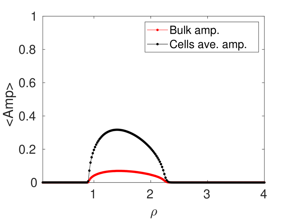
In terms of the cell population density $\rho$ , in Figure 13 we plot the numerically computed order parameter $R$ and the corresponding average amplitudes of predicted oscillations, as computed from the ODEs (4.0.1), for $1000$ cells. Since the cell population is fixed at $m=1000$ , increasing the population density $\rho$ corresponds to decreasing the area $|\Omega|$ of the 2-D bounded domain $\Omega$ . The results in Figure 13 are for the Sel’kov kinetic parameters $\mu=2$ , $\epsilon_{0}=0.15$ , the reaction-time parameter $\tau=0.5$ , and the permeabilities $k_{1}=10.0531$ and $k_{2}=2.5133$ . The remaining Sel’kov parameter value $\alpha$ was fixed at $\alpha=0.9$ for the identical cells, and was chosen uniformly from the interval $0.9220\leq\alpha\leq 0.9520$ for the defective cells. As seen from Figure 2, each cell has Sel’kov kinetic parameters that are chosen so that intracellular steady-state is linearly stable when there is no coupling to the bulk medium. From Figure 13 we observe that there are unique critical values of $\rho$ at which the order parameter $R$ switches from $0$ to $1$ (perfectly out of phase to perfect synchrony) and from $1$ to $0$ (perfect synchrony to perfectly out of phase). These transitions occur in a switch-like manner, in the sense that when intracellular oscillations emerge they all synchronize simultaneously. When $R$ switches from $0$ to $1$ , the synchronous intracellular oscillations that are triggered can be interpreted as a quorum sensing transition in the sense that it occurs for $1000$ cells only when the domain area $|\Omega|$ is small enough. Similarly, the cells desynchronize simultaneously as $\rho$ increases past a further threshold, leading to a linearly stable steady state. For identical cells, this linearly stable steady-state when $\rho$ exceeds a threshold was predicted theoretically in §4.1. Having two critical values of $\rho$ , labeled by $\rho_{1}$ and $\rho_{2}$ , at which the dynamics of the cells change state agrees with our earlier observation in Figure 12 that cell population density plays a dual role of initiating and then quenching intracelluar oscillations. When the cells are all identical, the critical population densities are $\rho_{1}=0.8$ and $\rho_{2}=2.77$ , when 600 of the cells are identical (remaining 400 are defective) we have $\rho_{1}=0.9$ and $\rho_{2}=2.34$ , and when only $100$ of the cells are identical (remaining 900 are defective) we have $\rho_{1}=1.14$ and $\rho_{2}=1.76$ . For any $\rho$ in $\rho_{1}\leq\rho<\rho_{2}$ , we have $R=1$ and perfect synchrony in the intracellular dynamics. On the other hand, when $\rho<\rho_{1}$ , we have $R=0$ so that the cells are either perfectly out of phase or there are no oscillations. This occurs when there are too few cells relative to the area of the domain, as there is insufficient secreted chemical from the cells to trigger synchronous oscillations. Similarly, $R=0$ when $\rho>\rho_{2}$ , since in this case the domain area is sufficiently small so much that the cells behave like a single effective cell, which has a linearly stable steady state.

In Figure 13 we observe that an increase in the relative proportion of defective cells in the population significantly alters the critical values $\rho_{1}$ and $\rho_{2}$ for which synchronous oscillations are triggered and quenched, respectively. As the number of defective cells increases, the range of $\rho$ that predicts perfect synchrony shrinks (see Figures 13(a), 13(b), and 13(c)), and so does the amplitudes of the predicted oscillations (see Figures 13(d), 13(e), and 13(f)). This shows that synchronous intracellular dynamics, resulting from effective communication between the cells, becomes more difficult to sustain as the relative number of defective cells increases.

5 Discussion

We have studied the emergence of oscillatory intracellular dynamics for a collection of $m$ small dynamically active disk-shaped signaling compartments, referred to as “cells”, that are coupled together through a scalar passive bulk diffusion field in a bounded 2-D domain. In our theoretical model, originating from [19] (see also [20] and [32]) and later extended and formalized in [9], each cell secretes across its boundary only one signaling chemical into the common bulk medium, while it receives feedback across its boundary from the entire collection of cells. This boundary efflux and influx of signaling material is regulated by permeability parameters. The resulting PDE-ODE model (1.0.1), given in dimensionless form in (2.1.1), was studied in the limit of a small common cell radius $\varepsilon\ll 1$ and in the limit where the bulk diffusion coefficient $D$ is asymptotically large, on the range $D\gg\mathcal{O}(\nu^{-1})\gg\mathcal{O}(1)$ where $\nu\equiv{-1/\log\varepsilon}\ll 1$ . In this limit, where the bulk region becomes well-mixed and the bulk concentration becomes spatially homogeneous, a matched asymptotic analysis was used to reduce the dimensionless PDE-ODE model into the system of ODEs (2.2.18) with global coupling. A similar reduction, but for identical cells, was done in [9].

For the specific case of Sel’kov reaction kinetics, we have used this ODE system to provide a detailed study of the emergence of intracellular oscillations in a collection of cells that is due to the cell-cell coupling through the bulk medium, and which otherwise would not occur for isolated cells. As such we have assumed that the Sel’kov kinetic parameters are chosen so that each cell is a conditional oscillator, and so its dynamics has only a stable steady-state when uncoupled from the bulk. For identical cells, the emergence of intracellular oscillations is found to arise via a Hopf bifurcation of the globally coupled system as parameters are varied.

One key focus has been to provide a detailed bifurcation study of the role of cell membrane permeabilites and the Sel’kov kinetic parameters on the emergence of intracellular oscillations. Our numerical bifurcation study using XPPAUT [6] has considered two main scenarios: one where all the cells are identical, and the other where there is a defector cell that is coupled to a group identical cells. A cell is considered defective if its Sel’kov kinetic parameters or permeabilities are different from those of the group of identical cells. Our results were presented in the form of one- and two-parameter global bifurcation diagrams of steady-states and periodic solution branches of the ODEs (2.2.18). Some highlights of the effect of a defector cell on a small group of identical cells include the following: Small changes in the influx rate of a single defective cell, relative to the common influx rate of the group, can act as a switch that extinguishes intracellular oscillations for the entire collection of cells (see Figures 3(c) and 3(d)). Intracellular oscillations of an entire group of cells can be extinguished by a single defective cell that reduces its efflux rate (see Figures 4(c) and 4(d)). Intracellular oscillations of an entire group of identical cells can be extinguished (see Figure 6) or triggered (see Figure 7) through increases or decreases, respectively, in the Sel’kov kinetic parameter $\alpha$ of one defective cell. A more detailed discussion of the effect of a defector cell on a small group of identical cells is given in §3.

Our second key focus was to use the ODE system (2.2.18) to study quorum sensing behavior associated with a large collection of either identical cells or a mixture of identical and defective cells. In terms of a cell density parameter, defined by $\rho\equiv{m/|\Omega|}$ , we showed that quorum sensing is characterized by the switch-like emergence of synchronous intracellular oscillations as $\rho$ crosses through a critical threshold $\rho_{1}$ (see Figures 12 and 13). Moreover, we showed that further increases in the cell density parameter eventually leads to a switch-like quenching of the oscillations when a second threshold density $\rho_{2}$ is reached. For the case of identical cells, we showed that these two thresholds $\rho_{1}$ and $\rho_{2}$ are Hopf bifurcation points associated with a cubic polynomial (see (4.1.8)), while the existence of the second threshold follows from (4.1.12). The qualitative explanation underlying the quenching threshold is that for large $\rho$ the collection of cells behaves like a single “effective” cell, which has no intracellular oscillations since it is a conditional Sel’kov oscillator. For two different mixtures of identical and defective cells, for which the Sel’kov kinetic parameter $\alpha$ was uniformly distributed in some interval, the Kuramoto order parameter in (4.2.1) was computed numerically to establish intervals in the cell density parameter $\rho$ where synchronous intracellular oscillations occur.

There are several possible extensions of our modeling framework and analysis that should be considered. One main direction would be to analyze (2.1.1) for the finite bulk diffusion regime $D={\mathcal{O}}(1)$ for an arbitrary collection of non-identical small cells in a bounded 2-D domain. In particular, it would be interesting to investigate the effect of various spatial factors, such as diffusion sensing and the role of cell-clustering (cf. [8]), on the emergence of intracellular oscillations for a collection of cells whose reaction kinetics are conditional Sel’kov oscillators. In this context, the spatial diffusion gradient and the overall spatial configuration of cells should determine which cells can effectively communicate and synchronize their dynamics. In particular, is a chimera-type state involving distinct intracellular oscillations for different cell-clusters within the entire group possible in this parameter regime?

Our PDE-ODE system (2.1.1) with Sel’kov reaction kinetics provides a simple conceptual model that predicts the switch-like emergence of intracellular oscillations with increasing cell density, known as quorum sensing, and this feature is qualitatively similar to that seen in many biological and chemical settings (cf. [4], [10], [12], [18], [14], [29], [28], [31], [30]). As a second main direction, it would be worthwhile to investigate triggered intracellular oscillations and quorum sensing behavior when the Sel’kov kinetics in our theoretical PDE-ODE system (2.1.1) are replaced with specific biologically-motivated reaction kinetics, such as the detailed model of [34] and [11] for the glycolytic pathway in yeast cells and the model of [18] for bacterial communication of Escherichia coli cells. In other settings, such as in the modeling of bioluminescence emitted by the marine bacterium Vibrio fischeri, the quorum sensing behavior of microbial cells due to an autoinducer bulk field does not involve the triggering of intracellular oscillations, but instead is believed to involve the sudden transition to a new stable steady-state (the bioluminescent state) as the cell population increases past a threshold (cf. [17]). It would be interesting to incorporate the intracellular signaling pathways of [17] into our PDE-ODE system (2.1.1) to show that quorum sensing in this context results from a saddle-node structure of equilibria and the sudden transition between stable states as the number of cells increases. Other modeling approaches to analyze quorum sensing behavior associated with sudden transitions between stable steady-states as the cell density increases past a threshold are given in [33] and [5].

Finally, other cell-cell communication problems mediated by a bulk diffusion field involve two-bulk diffusing species that mediate interactions between small signalling compartments. In this direction, it would be interesting to reframe the class of agent-based models considered in [24] for Turing pattern formation into an extended version of our PDE-ODE system (2.1.1) where there are now two-bulk diffusing species, consisting of an activator and an inhibitor field. For this scenario, it would be interesting to investigate, by using the permeabilities as bifurcation parameters, whether a Turing bifurcation can occur even when the activator and inhibitor bulk diffusion fields have very similar diffusion coefficients, as is typical in real-world biological systems.

Acknowledgements

Michael Ward gratefully acknowledges the financial support from the NSERC Discovery grant program.

Appendix A Non-dimensionalization of the coupled PDE-ODE model

In this appendix, the dimensional coupled PDE-ODE model (1.0.1) is non-dimensionalized. With $[z]$ denoting the dimension of $z$ , the dimensional units of the variables in this model are


$\displaystyle[\mathcal{U}]$	$\displaystyle=\frac{\text{moles}}{(\text{length})^{2}}\,,\qquad[\mu_{c}]=\text{moles}\,,\qquad[D_{B}]=\frac{(\text{length})^{2}}{\text{time}}\,,\qquad[k_{R}]=[k_{B}]=\frac{1}{\text{time}}\,,$	(A.0.1a)
$\displaystyle\quad[\boldsymbol{\mu}_{j}]$	$\displaystyle=\text{moles}\,,\qquad[\beta_{1,j}]=\frac{\text{length}}{\text{time}}\,,\qquad[\beta_{2,j}]=\frac{1}{\text{length}\times\text{time}}\quad\text{for}\quad j=1,\ldots,m\,.$	(A.0.1b)

We assume that the cells are circular with a common radius $R_{0}$ , which is small relative to the length-scale of the domain $L$ , and so we define a small parameter $\varepsilon={R_{0}/L}\ll 1$ . We then introduce dimensionless variables defined by

\displaystyle U=\frac{L^{2}}{\mu_{c}}\,\mathcal{U}\,,\qquad\boldsymbol{x}=\frac{\boldsymbol{X}}{L}\,,\qquad t=k_{R}\,T\,,\qquad\boldsymbol{u}_{j}=\frac{\boldsymbol{\mu}_{j}}{\mu_{c}}\,.

(A.0.2)

Observe that the dimensionless time-scale that is chosen is the time-scale for the reaction kinetics of the cells. By introducing (A.0.2) into (1.0.1), we obtain that the dimensionless bulk concentration satisfies


	$\displaystyle\frac{k_{R}}{k_{B}}\,U_{t}=D\Delta U-\,U\,,\qquad$	$\displaystyle\boldsymbol{x}\in\Omega\setminus\cup_{j=1}^{m}\Omega_{\varepsilon_{j}}\,;$	(A.0.3a)
	$\displaystyle\varepsilon\,D\,\partial_{n}U=\frac{\varepsilon\,\beta_{1,j}}{L\,k_{B}}\,\,U-\frac{\varepsilon\,\beta_{2,j}L}{k_{B}}\,\,u_{j}^{1}$	$\displaystyle\qquad\text{on}\quad\partial\Omega_{\varepsilon_{j}}\,;\qquad\partial_{n}U=0\quad\text{on}\quad\partial\Omega\,,$	(A.0.3b)
where $D\equiv D_{B}/(L^{2}\,k_{B})$ is the dimensionless bulk diffusivity, $\Omega_{\varepsilon_{j}}$ for $j=1,\dots,m$ are disks of a common radius $\varepsilon$ , and $\Delta$ is the Laplace operator with respect to $\boldsymbol{x}$ . This PDE for the dimensionless bulk concentration is coupled to the intracellular dynamics of the $j^{\text{th}}$ cell using the dimensionless integro-differential equation given by

	$\displaystyle\frac{\text{d}\boldsymbol{u}_{j}}{\text{d}t}=\boldsymbol{F}_{j}(\boldsymbol{u}_{j})+\frac{\boldsymbol{e}_{1}}{\varepsilon}\,\frac{k_{B}}{k_{R}}\,\int_{\partial\Omega_{\varepsilon_{j}}}\left(\frac{\varepsilon\,\beta_{1,j}}{L\,k_{B}}\,U-\frac{\varepsilon\,\beta_{2,j}L}{k_{B}}\,u_{j}^{1}\right)\,\,\text{d}S_{x}\,,$		(A.0.3c)

where we used $\text{d}S_{\boldsymbol{X}}=L\,\text{d}S_{\boldsymbol{x}}$ . In terms of the dimensionless variables

\displaystyle\tau\equiv\frac{k_{R}}{k_{B}}\,,\qquad D\equiv\frac{D_{B}}{L^{2}\,k_{B}}\,,\qquad d_{1,j}\equiv\frac{\varepsilon\,\beta_{1,j}}{L\,k_{B}}\,,\quad\text{and}\quad d_{2,j}\equiv\frac{\varepsilon\,\beta_{2,j}L}{k_{B}}\,,

(A.0.4)

the dimensionless form of the coupled PDE-ODE model (1.0.1) is given by


	$\displaystyle\tau\,U_{t}=D\Delta U-\,U\,,\qquad$	$\displaystyle\boldsymbol{x}\in\Omega\setminus\cup_{j=1}^{m}\Omega_{\varepsilon_{j}}\,;$	(A.0.5a)
	$\displaystyle\varepsilon\,D\,\partial_{n}U=d_{1,j}\,\,U-d_{2,j}\,\,u_{j}^{1}$	$\displaystyle\qquad\text{on}\quad\partial\Omega_{\varepsilon_{j}}\,;\qquad\partial_{n}U=0\quad\text{on}\quad\partial\Omega\,,$	(A.0.5b)
in the bulk region. This PDE is coupled to the intracellular dynamics of the $j^{\text{th}}$ cell through

	$\displaystyle\frac{\text{d}\boldsymbol{u}_{j}}{\text{d}t}=\boldsymbol{F}_{j}(\boldsymbol{u}_{j})+\frac{\boldsymbol{e}_{1}}{\varepsilon\,\tau}\,\,\int_{\partial\Omega_{\varepsilon_{j}}}\left(d_{1,j}\,U-d_{2,j}\,u_{j}^{1}\right)\,\,\text{d}S_{x}\,.$		(A.0.5c)

Appendix B Gallery of Numerical Simulations

Here, we present some numerical simulations of the reduced system of ODEs (2.2.18).

References

[1] K. L. Asfahl and M. Schuster. Social interactions in bacterial cell-cell signaling. FEMS Microbiology Reviews, 41(1):92–107, 2017.
[2] M. Chaplain, M. Ptashnyk, and M. Sturrock. Hopf bifurcation in a gene regulatory network model: Molecular movement causes oscillations. Math. Mod. Meth. Appl. Sci., 25(6):1179–1215, 2015.
[3] S. Danø, M. F. Madsen, and P. G. Sorensøn. Quantitative characterization of cell synchronization in yeast. Proceedings of the National Academy of Sciences, 104(31):12732–12736, 2007.
[4] S. De Monte, F. d’Ovidio, S. Danø, and P. G. Sørensen. Dynamical quorum sensing: Population density encoded in cellular dynamics. Proceedings of the National Academy of Sciences, 104(47):18377–18381, 2007.
[5] J. D. Dockery and J. P. Keener. A mathematical model for quorum sensing in pseudomonas aeruginosa. Bull Math Biol., 63(1):95–116, 2001.
[6] B. Ermentrout and Analyzing Simulating. Animating dynamical systems: A guide to xppaut for researchers and students (software, environments, tools). Society for Industrial and Applied Mathematics, 2002.
[7] K. Fujimoto and Sawai S. A design principle of group-level decision making in cell populations. PLoS Computational Biology, 9(6):e1003110, 2013.
[8] M. Gao, H. Zheng, Y. Ren, R. Lou, F. Wu, X. Yu, W. Liu, and X. Ma. A crucial role for spatial distribution in bacterial quorum sensing. Scientific reports, 6:34695, 2016.
[9] J. Gou and M. J. Ward. An asymptotic analysis of a 2-D model of dynamically active compartments coupled by bulk diffusion. Journal of Nonlinear Science, 26(4):979–1029, 2016.
[10] T. Gregor, K. Fujimoto, N. Masaki, and S. Sawai. The onset of collective behavior in social amoebae. Science, 328(5981):1021–1025, 2010.
[11] M. A. Henson, Müller D., and M. Reuss. Cell population modelling of yeast glycolytic oscillations. Biochem J., 368:433–446, 2002.
[12] K. Kamino, K. Fujimoto, and Sawai S. Collective oscillations in developing cells: Insights from simple systems. Develop. Growth Differ., 53:503–517, 2011.
[13] Y. Kuramoto. Self-entrainment of a population of coupled non-linear oscillators. In International symposium on mathematical problems in theoretical physics, pages 420–422. Springer, 1975.
[14] E. J. Leaman, B. Q. Geuther, and B. Behkam. Quantitative investigation of the role of intra-/intercellular dynamics in bacterial quorum sensing. ACS synthetic biology, 7(4):1030–1042, 2018.
[15] B. W. Li, X. Z. Cao, and C. Fu. Quorum sensing in populations of spatially extended chaotic oscillators coupled indirectly via a heterogeneous environment. Journal of Nonlinear Science, 27(6):1667–1686, 2017.
[16] B. W. Li, C. Fu, H. Zhang, and X. Wang. Synchronization and quorum sensing in an ensemble of indirectly coupled chaotic oscillators. Physical Review E, 86(4):046207, 2012.
[17] P. Melke, P. Sahlin, A. Levchenko, and H. Jonsson. A cell-based model for quorum sensing in heterogeneous bacterial colonies. PLoS Computational Biology, 6(6):e1000819, 2010.
[18] P. Mina, M. di Benardo, N. J. Savery, and K. Tsaneva-Atanasova. Modeling emergence of oscillations in communicating bacteria: a structured approach from one to many cells. J. Royal Society Interface, 10:20120612, 2012.
[19] J. Müller, C. Kuttler, B. A. Hense, M. Rothballer, and A. Hartmann. Cell–cell communication by quorum sensing and dimension-reduction. Journal of Mathematical Biology, 53(4):672–702, 2006.
[20] J. Müller and H. Uecker. Approximating the dynamics of communicating cells in a diffusive medium by ODEs — homogenization with localization. Journal of Mathematical Biology, 67(5):1023–1065, 2013.
[21] V. Nanjundiah. Cyclic AMP oscillations in dictyostelium discoideum: models and observations. Biophysical Chemistry, 72(1-2):1–8, 1998.
[22] J. Noorbakhsh, D. Schwab, A. Sgro, T. Gregor, and P. Mehta. Modeling oscillations and spiral waves in Dictyostelium populations. Phys. Rev. E., 91:062711, 2015.
[23] Nykamp D. Q. The idea of synchrony of phase oscillators. From Math Insight: http://mathinsight.org/synchrony_phase_oscillator_idea.
[24] E. M. Rauch and M. Millonas. The role of trans-membrane signal transduction in turing-type cellular pattern formation. J. Theor. Biol., 226:401–407, 2004.
[25] D. J. Schwab, A. Baetica, and P. Mehta. Dynamical quorum-sensing in oscillators coupled through an external medium. Physica D, 241(21):1782–1788, 2012.
[26] E. E. Sel’Kov. Self-oscillations in glycolysis 1. A simple kinetic model. European Journal of Biochemistry, 4(1):79–86, 1968.
[27] L. F. Shampine and M. W. Reichelt. The Matlab ODE suite. SIAM journal on scientific computing, 18(1):1–22, 1997.
[28] A. F. Taylor, M. Tinsley, and K. Showalter. Insights into collective cell behavior from populations of coupled chemical oscillators. Phys. Chemistry Chem Phys., 17(31):20047–20055, 2015.
[29] A. F. Taylor, M. Tinsley, F. Wang, Z. Huang, and K. Showalter. Dynamical quorum sensing and synchronization in large populations of chemical oscillators. Science, 323(5914):614–6017, 2009.
[30] M. R. Tinsley, A. F. Taylor, Z. Huang, and K. Showalter. Emergence of collective behavior in groups of excitable catalyst-loaded particles: Spatiotemporal dynamical quorum sensing. Phys. Rev. Lett., 102:158301, 2009.
[31] M. R. Tinsley, A. F. Taylor, Z. Huang, F. Wang, and K. Showalter. Dynamical quorum sensing and synchronization in collections of excitable and oscillatory catalytic particles. Physica D, 239(11):785–790, 2010.
[32] H. Uecke, J. Müller, and B. A. Hense. Individual-based model for quorum sensing with background flow. Bulletin of mathematical biology, 76(7):1727–1746, 2014.
[33] J. P. Ward, J. R. King, A. J. Koerber, P. Williams, J. M. Croft, and R. E. Sockett. Mathematical modelling of quorum sensing in bacteria. Mathematical Medicine and Biology, 18(3):263–292, 2001.
[34] J. Wolf and R. Heinrich. Effect of cellular interaction on glycolytic oscillations in yeast: a theoretical investigation. Biochem J., 345:321–334, 2000.