Yokohama National University,
Hodogaya, Yokohama, 240-8501, Japan
Localization in quantum walks with periodically arranged coin matrices
Abstract
There is a property called localization, which is essential for applications of quantum walks. From a mathematical point of view, the occurrence of localization is known to be equivalent to the existence of eigenvalues of the time evolution operators, which are defined by coin matrices. A previous study proposed an approach to the eigenvalue problem for space-inhomogeneous models using transfer matrices. However, the approach was restricted to models whose coin matrices are the same in positions sufficiently far to the left and right, respectively. This study shows that the method can be applied to extended models with periodically arranged coin matrices. Moreover, we investigate localization by performing the eigenvalue analysis and deriving their time-averaged limit distribution.
1 Introduction
The study of quantum walks, which began in the early 2000s [1, 2], has spread and attracted much attention, especially for its applications in quantum information [3, 4, 5, 6, 7, 8]. One of the most characteristic properties of the quantum walk is localization, an essential property for manipulating particles. Numerical and theoretical analyses have been actively conducted, and we are particularly interested in the mathematical analysis of localization [9, 10, 11, 8, 12, 13]. It has been known that localization occurs in various quantum walk models. This study focuses on one-dimensional two-state quantum walks, which are considered the fundamental discrete-time quantum walks.
From a mathematical point of view, the investigation of localization can be regarded as an eigenvalue problem. This is because the occurrence of localization is equivalent to the existence of eigenvalues of the time evolution operator, and the corresponding eigenvectors are related to how likely the walker localizes [12, 14]. In a previous study [15], an eigenvalue analysis method using the transfer matrix was proposed. The eigenvalue analysis was performed for two-phase quantum walks with one defect, including a one-defect model where the time evolution differs at the origin and a two-phase model where the time evolution differs in the negative and positive parts, respectively. The localization phenomenon in the one-defect model has been used in quantum search algorithms [16, 3, 17], and the relationship between topological insulators and localization in the two-phase quantum walk has attracted much attention [18, 19]. Several other studies also used transfer matrices for deriving stationary measures [20, 21]. Furthermore, a previous study [14, 22] showed that the method could be applied to a more general model with a finite number of defects, which satisfies the following conditions:
where and are integers, and denotes the coin matrix determining the time evolution in the position . Models with periodic coin matrices have also been actively studied [23, 24, 25]. In particular, the model with self-duality studied in [25] is inspired by the well-studied Aubry-André model [26], and the Fourier transform method was applied. However, our approach can extend the discussion to models that cannot be handled by the Fourier transform method and simplify the eigenvalue problem since we only need to deal with 2 2 (transfer) matrices instead of the large matrix. In this study, we consider a two-phase periodic model with a finite number of defects that includes all of the above important models; the model has and different coin matrices arranged periodically in positions and , respectively.
This paper is organized as follows. In Section 2, we define our model with periodically arranged coin matrices and its transfer matrix. This section also shows that the eigenvalue analysis via transfer matrix is applicable for the model. The necessary and sufficient condition for the eigenvalue problem is given in Theorem 2.3. Also, further discussion about the time-averaged limit distribution using eigenvalues and eigenvectors is provided. With the main theorem, Section 3 focuses on analyzing concrete eigenvalues for more specific models, which can be seen as natural generalizations of homogeneous, one-defect, and two-phase models to periodic models.
2 Definitions and method
Firstly, we introduce two-state quantum walks on the integer lattice . The Hilbert space is given as defined by
where denotes the set of complex numbers. For , we write , where is the transpose operator. The time evolution operator is defined by the product of a coin operator on and a shift operator on . Here, and are defined by
where is a sequence of unitary matrices called coin matrices. We define where , then the periodicities of the model are defined by for positions and for positions , where is the set of positive integers. For , we define by remainder of divided by , that is,
We treat the model whose coin matrices satisfy the following:
The model has a finite number of defects in and periodic coin matrices for each of and . Here, we write as follows:
with and for .
We let denote the initial state of the model. Then, the probability distribution at time is defined by
where is the set of non-negative integers. Here, we say that the quantum walk model exhibits localization if there exists an initial state and a position satisfying
As a well-known fact that the quantum walk model exhibits localization if and only if the time evolution operator has an eigenvalue [12], which means that there exists and such that
Let denotes the set of eigenvalues of henceforward. Subsequently, let be a unitary operator on defined by
for . Here the inverse of is given as
Furthermore, for , and , we introduce the transfer matrix as followings:
We abbreviate the transfer matrix as and as henceforward. Here, satisfies if and only if satisfies the following equation for all :
| (1) |
For more details, see [15]. In this paper, we define notation for the products of matrices by the following:
For and , we define as follows:
where and This can be rewritten as
| (2) |
with
for Here, is a map constructed by transfer matrices, where satisfies equation (1) (but not necessarily satisfies ). For , has as a parameter. We let be a set of all possible obtained by varying :
Corollary 2.1.
Let , if and only if there exists such that , and associated eigenvector of becomes .
Note that where but not necessarily is the stationary measure of the quantum walk studied in [27, 28, 21, 20, 29]. We define sign function for real numbers as follows:
Then, two eigenvalues of can be written as expressed as below:
where . Note that the eigenvalues are independent of .
Corollary 2.2.
is a real number.
Proof.
Let
Here, holds for all , which implies that holds for all . Also, holds, thus we have and becomes a real number.
Subsequently, since for
holds, which also means . From Corollary 2.2, we know that and hold, and we have the main theorem.
Theorem 2.3.
For , if and only if the following two statements hold:
Proof.
From Corollary 2.1, if and only if there exists such that given by satisfies . If , both and become 1. Since is given as (2), we have for all . Therefore, the first condition is necessary for . Next, we assume that , then and hold. Thus, from (2), satisfies if and only if there exists such that
for all and
for all . Here denotes “if and only if”. However,
holds for all and
holds for all . Thus, the conditions can be summarized in the second condition of the theorem. Therefore, the statement is proved. ∎
This theorem implies that the eigenvalue problem is to find the solution of a single equation obtained from the second condition of the theorem in the range of . We can also see that if , the associated eigenvector is given as where
with
Furthermore, we can quantitatively evaluate localization by deriving time-averaged limit distribution defined by
The time-averaged limit distribution can be calculated by the eigenvectors of [12]. For multiplicity and complete orthonormal basis , the following holds:
Here, we show some important facts for calculating .
Lemma 2.4.
has at most a finite number of eigenvalues with the multiplicity of 1, that is,
and
Proof.
By definition and Theorem 2.3, If , then
becomes zero matrix and . This is clearly a contradiction. By similar discussion for we have
Also,
is immediately shown. Subsequently, we can see that
Furthermore, has to be a root of the equation
Hence, the number of satisfying the above equation is finite, and we complete the proof. ∎
Therefore, can be written as
| (3) |
3 Results
3.1 Homogeneously periodic model
Proposition 3.1.
Let and . The coin matrices become
where . Then, the model does not exhibit localization, that is, .
Proof.
From (3), we can also see that the time-averaged limit distribution is always for all positions . As a remark, when for some (excluded case), the model exhibits localization in the finite interval since the quantum walker is reflected at position where . This fact is described in detail by [25] as a lemma for the specific case
where is a rational number. With our Proposition 3.1, we can say that their lemma claims the only case in which the model exhibits localization. Our result contributes to solving one of the open problems mentioned in [25] for the general coin matrices. Moreover, note that when , and if initial state satisfies for all odd positions or all even positions , this model can be regarded as a time-dependent two-period quantum walks studied in [30].
3.2 Periodic model with one-defect
Next, we consider a one-defect model with a different coin matrix acts only on the origin in the homogeneously periodic model defined above. This is an extension of the usual one-defect model treated in previous study [15] by replacing coin matrices in positive and negative parts with periodic coins. The model is given by setting , and the transfer matrix can also be written as . Then, coin matrices become
We get the analytical result for this model with . From Theorem 2.3, if and only if followings hold:
where denotes the real part of a complex number.
Proposition 3.2.
Let . Then,
where

3.3 Two-phase periodic model
Next, we consider a two-phase model where two different groups of periodic coin matrices act on each of non-negative and negative parts, respectively. This is an extension of the usual two-phase model treated in previous study [15] by replacing coin matrices in each of non-negative and negative parts with periodic coins. The model is given by setting . We write
for . Then, the coin matrices become
where . We get analytical results for this model with . From Theorem 2.3, if and only if followings hold:
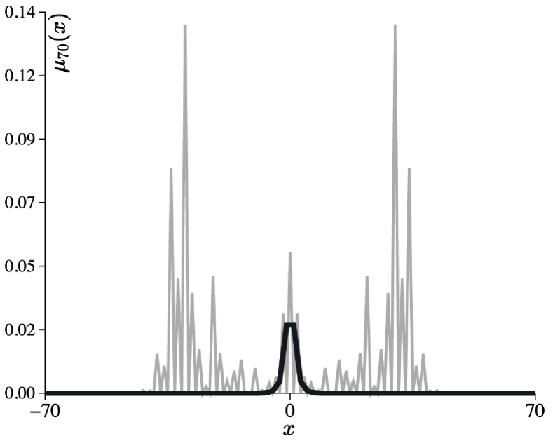
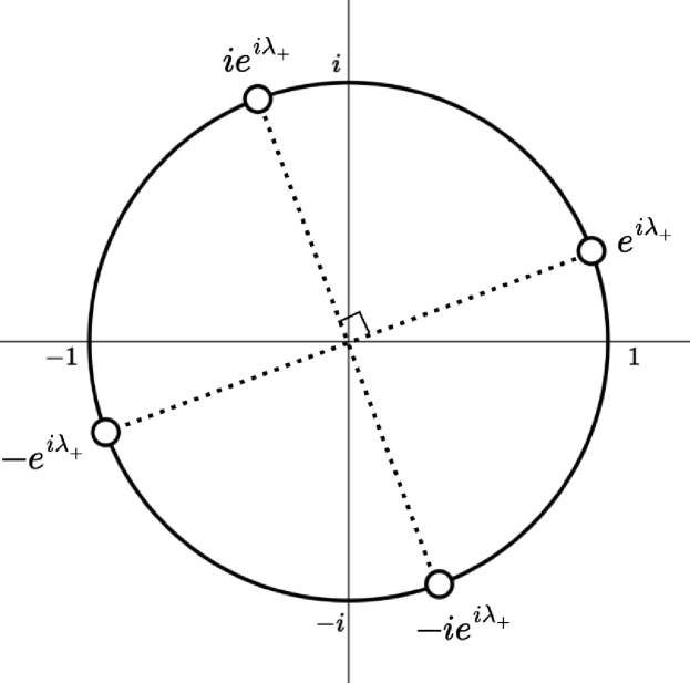
Proposition 3.3.
Let , Then, if and only if and and becomes
where
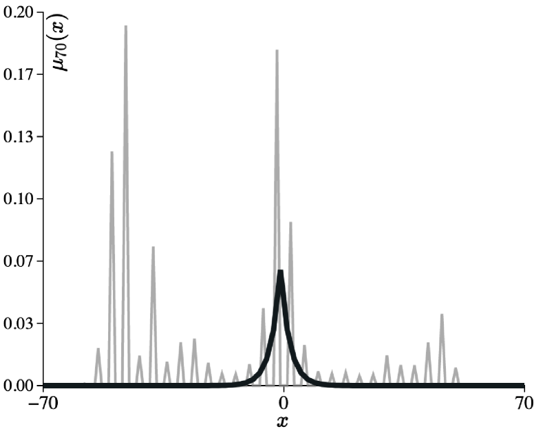
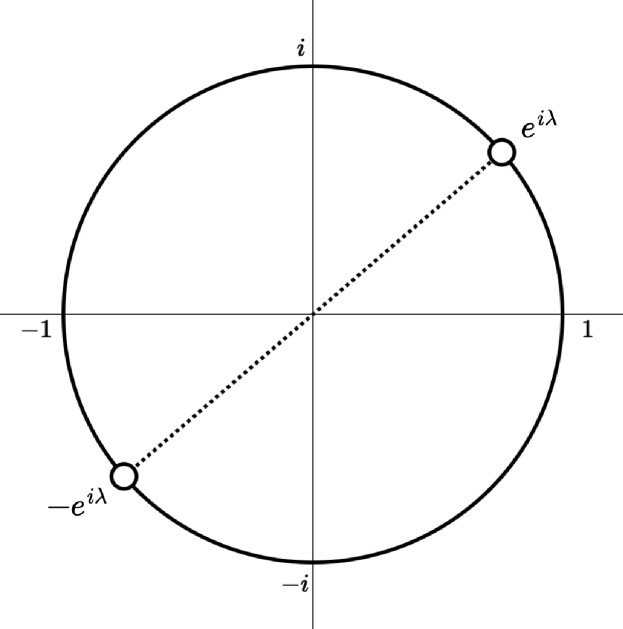
Proposition 3.4.
Let , Then, if and only if and . In this case,
where
4 Summary
In previous studies [15, 14], the eigenvalue analysis using a transfer matrix was performed for a model with homogeneous coin matrices in positions sufficiently far to the left and right, respectively, which include one-defect and two-phase models. This study focuses on the eigenvalue problem for a more generalized model in which the coin matrices are arranged periodically in positions sufficiently far to the left and right, respectively. Theorem 2.3 is the main theorem, and it successfully provides the necessary and sufficient conditions for the eigenvalue problem. Furthermore, we showed in Lemma 2.4 that the model has at most a finite number of eigenvalues with the multiplicity of 1, and we further discussed about the analytical formulation of the time-averaged limit distribution. Based on the main theorem, we considered the more specific models, which can be seen as generalizations of homogeneous, one-defect, and two-phase models. Proposition 3.1 showed that if periodic coin matrices are arranged homogeneously, the model does not exhibit localization. Finally, Propositions 3.2, 3.3 and 3.4 derived the concrete eigenvalues for specific models with periodicity 2.
For future research, further analysis using the transfer matrix for more general or different types of models, such as higher-dimensional and split-step [18] quantum walks, would be interesting.
Acknowledgements
The author expresses sincere thanks and gratitude to Kei Saito for helpful comments and discussion.
References
- [1] Andris Ambainis et al. “One-dimensional quantum walks” In Proceedings of the thirty-third annual ACM symposium on Theory of computing Hersonissos, Greece: Association for Computing Machinery, 2001, pp. 37–49
- [2] Norio Konno “Quantum Random Walks in One Dimension” In Quantum Inf. Process. 1.5, 2002, pp. 345–354
- [3] Andrew M Childs and Jeffrey Goldstone “Spatial search by quantum walk” In Phys. Rev. A 70.2 American Physical Society, 2004, pp. 022314
- [4] Andrew M Childs “Universal computation by quantum walk” In Phys. Rev. Lett. 102.18, 2009, pp. 180501
- [5] Neil B Lovett et al. “Universal quantum computation using the discrete-time quantum walk” In Phys. Rev. A 81.4, 2010, pp. 042330
- [6] Andrew M Childs, David Gosset and Zak Webb “Universal computation by multiparticle quantum walk” In Science 339.6121, 2013, pp. 791–794
- [7] P R N Falcão et al. “Universal dynamical scaling laws in three-state quantum walks” quant-ph/2108.10275
- [8] Takuya Machida “Limit theorems of a 3-state quantum walk and its application for discrete uniform measures” In Quantum Inf. Comput. 15.5&6, 2015, pp. 406–418
- [9] M J Cantero, F A Grünbaum, L Moral and L Velázquez “The CGMV method for quantum walks” In Quantum Inf. Process. 11.5 Springer ScienceBusiness Media LLC, 2012, pp. 1149–1192
- [10] Shimpei Endo, Takako Endo, Takashi Komatsu and Norio Konno “Eigenvalues of Two-State Quantum Walks Induced by the Hadamard Walk” In Entropy 22.1, 2020, pp. 127
- [11] Norio Inui and Norio Konno “Localization of multi-state quantum walk in one dimension” In Phys. A: Stat. Mech. Appl. 353, 2005, pp. 133–144
- [12] Etsuo Segawa and Akito Suzuki “Generator of an abstract quantum walk” In Quantum Stud.: Math. Found. 3.1, 2016, pp. 11–30
- [13] Antoni Wójcik et al. “Trapping a particle of a quantum walk on the line” In Phys. Rev. A 85.1 American Physical Society, 2012, pp. 012329
- [14] Chusei Kiumi and Kei Saito “Strongly trapped space-inhomogeneous quantum walks in one dimension” math-ph/2105.10962
- [15] Chusei Kiumi and Kei Saito “Eigenvalues of two-phase quantum walks with one defect in one dimension” In Quantum Inf. Process. 20.5 Springer ScienceBusiness Media LLC, 2021, pp. 171
- [16] Neil Shenvi, Julia Kempe and K Birgitta Whaley “Quantum random-walk search algorithm” In Phys. Rev. A 67.5 American Physical Society, 2003, pp. 052307
- [17] Andris Ambainis, Julia Kempe and Alexander Rivosh “Coins make quantum walks faster” In Proceedings of the sixteenth annual ACM-SIAM symposium on Discrete algorithms Vancouver, British Columbia: Society for IndustrialApplied Mathematics, 2005, pp. 1099–1108
- [18] Takuya Kitagawa, Mark S Rudner, Erez Berg and Eugene Demler “Exploring topological phases with quantum walks” In Phys. Rev. A 82.3 American Physical Society, 2010, pp. 033429
- [19] Takako Endo, Norio Konno and Hideaki Obuse “Relation between two-phase quantum walks and the topological invariant” In Yokohama Math. J. 64, 2020
- [20] Hikari Kawai, Takashi Komatsu and Norio Konno “Stationary measure for two-state space-inhomogeneous quantum walk in one dimension” In Yokohama Math. J. 64, 2018, pp. 111–130
- [21] Hikar Kawai, Takashi Komatsu and Noriko Konno “Stationary measures of three-state quantum walks on the one-dimensional lattice” In Yokohama Math. J. 63, 2017, pp. 59–74
- [22] Chusei Kiumi “Eigenvalues of two-phase three-state quantum walks with one defect” math-ph/2111.14300
- [23] Noah Linden and James Sharam “Inhomogeneous quantum walks” In Phys. Rev. A 80.5 APS, 2009, pp. 052327
- [24] Rashid Ahmad, Uzma Sajjad and Muhammad Sajid “One-dimensional quantum walks with a position-dependent coin” In Commun. Math. Phys. 72.6 IOP Publishing, 2020, pp. 065101
- [25] Yutaka Shikano and Hosho Katsura “Localization and fractality in inhomogeneous quantum walks with self-duality” In Phys. Rev. E 82 American Physical Society, 2010, pp. 031122
- [26] S Aubry and G André “Analyticity breaking and Anderson localization in incommensurate lattices” In Ann. Israel Phys. Soc. 3, 1980, pp. 18
- [27] Takako Endo and Norio Konno “The stationary measure of a space-inhomogeneous quantum walk on the line” In Yokohama Math. J. 60, 2014, pp. 33–47
- [28] Caishi Wang, Xiangying Lu and Wenling Wang “The stationary measure of a space-inhomogeneous three-state quantum walk on the line” In Quantum Inf. Process. 14.3 Springer ScienceBusiness Media LLC, 2015, pp. 867–880
- [29] Takako Endo, Takashi Komatsu, Norio Konno and Tomoyuki Terada “Stationary measure for three-state quantum walk” In Quantum Inf. Comput. 19.11&12 Rinton Press, 2019, pp. 901–912
- [30] Takuya Machida and Norio Konno “Limit Theorem for a Time-Dependent Coined Quantum Walk on the Line” In Natural Computing Springer Japan, 2010, pp. 226–235