Localization-delocalization Transition in an electromagnetically induced photonic lattice

Localized light can be used as a versatile tool for various manipulation and processing in optical information. It thus can be considered as one of the foundation for information dissemination. Past studies show that lots of promising methods, such as designing the optical localization propagation in optical fibers, utilizing artificial periodic structures in the photonic crystal and constructing random structures with Anderson localization effect, can implement the light localization Akahane et al. (2003); Park et al. (2004); Joannopoulos et al. (2008); Smith et al. (2004); Schurig et al. (2006); Han et al. (2014). In particular, one of the key ingredients of these schemes is to engineer the spatial characteristics of the optical medium, which shows unprecedented capabilities in controlling the flow of light as well as matter wavesHu et al. (2005); Zhang and Liu (2008); Bhandari (1997); Lu et al. (2014); Ozawa et al. (2019).

Recently, another distinct approach to generate spatially periodic structures via the electromagnetically induced transparency (EIT) scheme Ling et al. (1998), either in hot atomic vapours Sheng et al. (2015); Zhang et al. (2018); Yuan et al. (2019) or ultracold atoms Radwell et al. (2015); Yang et al. (2020), has attracted considerable attention. Many intriguing phenomena, such as optical lattice solitons Fleischer et al. (2003); Michinel et al. (2006); Zhang et al. (2011), photon-atom bound state Longo et al. (2010), photonic Floquet topological insulators Rechtsman et al. (2013) and optical analogs of quantum random walks Peruzzo et al. (2010), have been explored.

In this work, we propose a four-level tripod-type scheme in atomic ensembles to generate an electromagnetically induced photonic moiré lattice Wang et al. (2020); Fu et al. (2020) through the EIT mechanism. By taking advantage of the tunable atomic coherence, it is shown that the moiré pattern is highly flexible via changing the twist angle between two superimposed periodic patterns with square primitive. Both periodic (commensurable) and aperiodic (incommensurable) structure can be achieved. Interestingly, we find a LDT of the light propagating in the aperiodic photonic moiré lattice, which manifests the typical flat-band feature of the moire lattice.

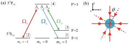
Let us take ${}^{87}\rm{Rb}$ atomic system as an example to show our proposed four-level tripod-type scheme, which is schematically presented in Fig.1(a). The signal, coupling, pump fields drive the transitions $|1\rangle\to|4\rangle,|2\rangle\to|4\rangle,|3\rangle\to|4\rangle$, respectively, where $|1\rangle$, $|2\rangle$, $|3\rangle$ can be chosen from $\mathrm{5^{2}S_{1/2}}$ state of ${}^{87}\rm{Rb}$, such as $|F=1,m_{F}=\pm 1\rangle$ and $|F=2,m_{F}=1\rangle$, while $|4\rangle$ can be selected from $\mathrm{5^{2}P_{1/2}}$ state, such as $|F^{\prime}=1,m_{F}=0\rangle$. Here we consider both the signal and pump beams are injected into atomic ensemble along the z-axis. The coupling field is consisted of two groups of orthogonalized paired-beams paraxially propagating along the $z$-direction.

Under the rotating-wave approximation, the density-matrix equations for our proposed 4-level tripod-type atomic system can be expressed as Wang et al. (2014)

	$\displaystyle\dot{\rho}_{11}=$	$\displaystyle-\frac{i}{2}\Omega_{s}\rho_{14}+\frac{i}{2}\Omega_{s}^{*}\rho_{41}+\Gamma_{41}\rho_{44}$
	$\displaystyle\dot{\rho}_{22}=$	$\displaystyle-\frac{i}{2}\Omega_{c}\rho_{24}+\frac{i}{2}\Omega_{c}^{*}\rho_{42}+\Gamma_{42}\rho_{44}$

	$\displaystyle\dot{\rho}_{33}=$	$\displaystyle-\frac{i}{2}\Omega_{p}\rho_{34}+\frac{i}{2}\Omega_{p}^{*}\rho_{34}\rho_{43}+\Gamma_{43}\rho_{44}$
	$\displaystyle\dot{\rho}_{44}=$	$\displaystyle\frac{i}{2}(\Omega_{s}\rho_{14}-\Omega_{s}^{*}\rho_{41})+\frac{i}{2}(\Omega_{c}\rho_{24}-\Omega_{c}^{*}\rho_{42})$
		$\displaystyle+\frac{i}{2}(\Omega_{p}\rho_{34}-\Omega_{p}^{*}\rho_{43})-\Gamma\rho_{44}$
	$\displaystyle\dot{\rho}_{21}=$	$\displaystyle i(\Delta_{s}-\Delta_{c})\rho_{21}+\frac{i}{2}\Omega_{c}^{*}\rho_{41}-\frac{i}{2}\Omega_{s}\rho_{24}$
	$\displaystyle\dot{\rho}_{31}=$	$\displaystyle i(\Delta_{s}-\Delta_{p})\rho_{31}+\frac{i}{2}\Omega_{p}^{*}\rho_{41}-\frac{i}{2}\Omega_{s}\rho_{34}$
	$\displaystyle\dot{\rho}_{41}=$	$\displaystyle\frac{i}{2}\Omega_{s}\rho_{11}+\frac{i}{2}\Omega_{c}\rho_{21}+\frac{i}{2}\Omega_{p}\rho_{31}-\frac{i}{2}\Omega_{s}\rho_{44}$
		$\displaystyle+i\Delta_{s}\rho_{41}-\frac{\Gamma}{2}\rho_{41}$
	$\displaystyle\dot{\rho}_{32}=$	$\displaystyle i(\Delta_{c}-\Delta_{p})\rho_{32}+\frac{i}{2}\Omega_{p}^{*}\rho_{42}-\frac{i}{2}\Omega_{c}\rho_{34}$
	$\displaystyle\dot{\rho}_{42}=$	$\displaystyle\frac{i}{2}\Omega_{s}\rho_{12}+\frac{i}{2}\Omega_{c}\rho_{22}+\frac{i}{2}\Omega_{p}\rho_{32}-\frac{i}{2}\Omega_{c}\rho_{44}$
		$\displaystyle+i\Delta_{c}\rho_{42}-\frac{\Gamma}{2}\rho_{42}$
	$\displaystyle\dot{\rho}_{43}=$	$\displaystyle\frac{i}{2}\Omega_{s}\rho_{13}+\frac{i}{2}\Omega_{c}\rho_{23}+\frac{i}{2}\Omega_{p}\rho_{33}-\frac{i}{2}\Omega_{p}\rho_{44}$
		$\displaystyle+i\Delta_{p}\rho_{43}-\frac{\Gamma}{2}\rho_{43}$		(1)

where $\Gamma_{nm}$ is the natural decay rate between level $|n\rangle$ and $|m\rangle$ and $\Gamma=\Gamma_{41}+\Gamma_{42}+\Gamma_{43}$. $\Omega_{s}=\mu_{41}E_{s}/\hbar$, $\Omega_{c}=\mu_{42}E_{c}/\hbar$ and $\Omega_{p}=\mu_{43}E_{p}/\hbar$ are Rabi frequencies of signal, coupling and pump fields, where $\mu_{ij}$ is the electric dipole matrix element related to the atomic transition between $|i\rangle$ and $|j\rangle$. $E_{s(c,p)}$ is the strength of corresponding electric field. $\Delta_{s}=\omega_{s}-\omega_{14}$, $\Delta_{c}=\omega_{c}-\omega_{24}$ and $\Delta_{p}=\omega_{p}-\omega_{34}$ denote the frequency detunings. Since the signal field is much weaker than both coupling and pump fields, from Eq .(II) we can obtain the following relations

	$\displaystyle\rho_{21}$	$\displaystyle=\frac{-\Omega_{c}^{*}/2}{\Delta_{s}-\Delta_{c}}\rho_{41}$
	$\displaystyle\rho_{31}$	$\displaystyle=\frac{-\Omega_{p}^{*}/2}{\Delta_{s}-\Delta_{p}}\rho_{41}.$		(2)

Substituting Eq .(II) into Eq .(II), $\rho_{41}$ can be solved as

$$\rho_{41}=-\left[(\Delta_{s}+\frac{i\Gamma}{2})+\frac{|\Omega_{c}|^{2}/4}{\Delta_{c}-\Delta_{s}}+\frac{|\Omega_{p}|^{2}/4}{\Delta_{p}-\Delta_{s}}\right]^{-1}\frac{\Omega_{s}}{2}$$

(3)

The susceptibility of atomic medium can be determined through the following formula

	$\displaystyle\chi=$	$\displaystyle 2N\mu_{14}\rho_{41}/\epsilon_{0}E_{s}$		(4)
	$\displaystyle=$	$\displaystyle\frac{-N|\mu_{14}|^{2}}{\epsilon_{0}}\left[(\Delta_{s}+\frac{i\Gamma}{2})+\frac{|\Omega_{c}|^{2}/4}{\Delta_{c}-\Delta_{s}}+\frac{|\Omega_{p}|^{2}/4}{\Delta_{p}-\Delta_{s}}\right]^{-1}$

where $N$ is the atomic density. The refractive index can be obtained via the relation $n=\sqrt{1+\chi}\approx 1+\chi/2$. From Eq .(4), one can notice that the spatial profile of the susceptibility is highly dependent on the distribution of the coupling fields, and thus can produce various structures by shaping them. To show that, here we consider that the coupling fields are consisted of two groups of orthogonalized paired-standing waves paraxially propagating along the z-axis (captured by a small angle $\phi$ to the z-axis), as depicted in Fig.1(b) by the solid and dashed lines, respectively.

The two groups of orthogonalized paired-standing waves can form two superimposed square patterns. And the total spatial pattern is highly tunable through changing the twisted angle $\theta$ as shown in Fig.1(b). To be more specific, the standing waves as shown in Fig.1(b) can be expressed as

	$\displaystyle\vec{E}_{c1}(\vec{r},t)$	$\displaystyle=E_{c}^{\prime}\cos k_{0}x[e^{i(k_{z}z-\omega_{c}t)}\hat{x}+e^{i(k_{z}z-\omega_{c}t-\pi/2)}\hat{y}]$
	$\displaystyle\vec{E}_{c2}(\vec{r},t)$	$\displaystyle=E_{c}^{\prime}\cos k_{0}y[e^{i(k_{z}z-\omega_{c}t+\pi/2)}\hat{x}+e^{i(k_{z}z-\omega_{c}t)}\hat{y}]$
	$\displaystyle\vec{E}_{c3}(\vec{r},t)$	$\displaystyle=E_{c}^{\prime\prime}\cos k_{0}x^{\prime}[e^{i(k_{z}z-\omega_{c}t)}\hat{x}^{\prime}+e^{i(k_{z}z-\omega_{c}t-\pi/2)}\hat{y}^{\prime}]$
	$\displaystyle\vec{E}_{c4}(\vec{r},t)$	$\displaystyle=E_{c}^{\prime\prime}\cos k_{0}y^{\prime}[e^{i(k_{z}z-\omega_{c}t+\pi/2)}\hat{x}^{\prime}+e^{i(k_{z}z-\omega_{c}t)}\hat{y}^{\prime}]$		(5)

where $k_{z}=k_{c}\cos\phi$ and $k_{0}=k_{c}\sin\phi$. Unit vectors $\hat{x}^{\prime},\hat{y}^{\prime}$ are related to $\hat{x},\hat{y}$ via the relation $\left[x^{\prime},y^{\prime}\right]^{\mathsf{T}}=S\cdot\left[x,y\right]^{\mathsf{T}}$, where $S=[\cos\theta,-\sin\theta;\sin\theta,\cos\theta]$ is the operator of two dimensional rotation. Therefore, the intensity of coupling field can be expressed as

	$\displaystyle\left|E_{c}(x,y)\right|^{2}=$	$\displaystyle 2E_{c}^{\prime 2}\Big{|}(\cos k_{0}y\cdot\hat{x}+\cos k_{0}x\cdot\hat{y})$
	$\displaystyle+$	$\displaystyle\alpha(\cos k_{0}y^{\prime}\cdot\hat{x}^{\prime}+\cos k_{0}x^{\prime}\cdot\hat{y}^{\prime})\Big{|}^{2}$		(6)

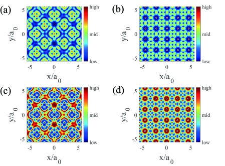
where $\alpha=E_{c}^{\prime\prime}/E_{c}^{\prime}$. As shown in Fig.2, when varying the twisted angle $\theta$ and amplitude ratio $\alpha$, the interference of coupling fields will produce different spatial pattern and induce an effective 2D photonic lattice in $xy$ plane. For instance, the periodic structure of refractive index lattice is produced when $\theta$ is a Pythagorean angle, e.g., $\theta=\arctan 4/3$ (see Fig.2 (b) and (d)), otherwise, the aperiodic structure is induced, e.g., $\theta=\pi/6$ (see Fig.2 (a) and (c))

In the following, we will demonstrate the effect of the spatial profiles of our proposed refractive index lattice through investigating the light propagation within it. The propagation of signal beam $\vec{E}_{s}(\vec{r},t)$ in the atomic medium is governed by the following electric field wave equation

$$\nabla^{2}\vec{E}_{s}+\frac{\omega_{s}^{2}}{c^{2}}\epsilon(\vec{r})\vec{E}_{s}=0$$

(7)

where $\epsilon=1+\chi$ is the relative dielectric constant. We then rewrite $\vec{E}_{s}(\vec{r},t)$ as $\vec{E}_{s}(\vec{r},t)=\psi(\vec{r})[\exp{(ik_{s}z-i\omega_{s}t)}\hat{x}+\exp{(ik_{s}z-i\omega_{s}t+\pi/2)}\hat{y}]$ with $\psi(\vec{r})$ being the field amplitude. Then, from Eq. (7) a Schrödinger-type equation of $\psi(\vec{r})$ can be obtained

$$i\frac{\partial}{\partial z}\psi=-\frac{1}{2k_{s}}\left(\frac{\partial^{2}}{\partial x^{2}}+\frac{\partial^{2}}{\partial y^{2}}\right)\psi-\frac{k_{s}\Delta n(x,y)}{n_{0}}\psi$$

(8)

where $\Delta n(x,y)\approx\chi/2$ and $k_{s}=2\pi n_{0}/\lambda_{s}$ being the wave vector of signal beam. $n_{0}$ is ambient refractive index.

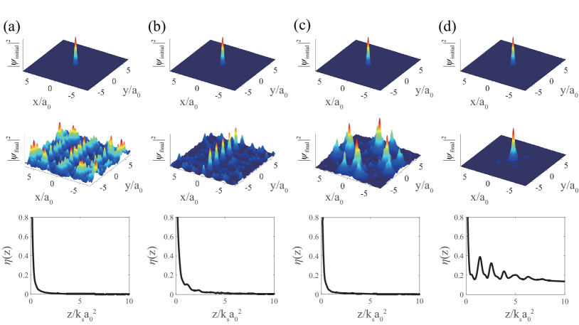
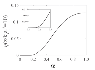
To investigate the light propagation in the refractive index lattices as shown in Fig.2, we initialize the signal beam as a Gaussion wavepacket and numerically simulate its propagation. As shown in Fig.3, when $\theta$ is chosen as a Pythagorean angle, for instance, $\theta=\arctan 4/3$, the refractive index lattices possess a spatially periodic structure and the initial Gaussion wavepacket displays the delocalization behavior for arbitrary amplitude ratio $\alpha$ of the two superimposed periodic patterns. When the refractive index lattices possess a spatial aperiodic structure, for instance, $\theta=\pi/6$, we find that there is a threshold of $\alpha$. Below that threshold, as shown in Fig.3 (c), the light propagation still shows the delocalization behavior. However, if $\alpha$ exceeds the threshold, as shown in Fig.3 (d), the signal beam turns out to be localized. Therefore, there is a localization-delocalization transition (LDT) in aperiodic moiré lattice, when tuning the amplitudes of the two superimposed periodic patterns. To quantitatively analyze the LDT here, we introduce the factor inverse participation ratio (IPR)Evers and Mirlin (2000) defined as $\eta(z)=\int|\psi(\vec{r})|^{4}dxdy/\left(\int|\psi(\vec{r})|^{2}dxdy\right)^{2}$. The localized behavior can be captured by the non-zero IPR. As shown in Fig.4, the threshold of amplitude ratio in the aperiodic moiré lattice separating two distinct regimes in the LDT can be determined by the non-zero point of IPR when varying $\alpha$.

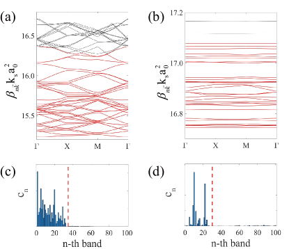
To understand the localization of light in aperiodic moiré lattice, we calculate its single-particle dispersion relation through approximating the non-Pythagorean twist angle by a Pythagorean one Wang et al. (2020). For instance, here we use $\theta=\arctan{(120/209)}$ to approximate $\theta=\pi/6$. Under such an approximation, the single-particle dispersion of aperiodic lattice can be obtained by the plane-wave expansion method through introducing the Bloch basis $\psi_{n\vec{k}}=\sum_{\vec{G}}u_{n\vec{k},\vec{G}}|\vec{k}+\vec{G}\rangle$ with the Bloch vector $\vec{k}$ and reciprocal lattice vector $\vec{G}$. Here $n$ labels the band index. Then, the single-particle dispersion relation can be obtained through solving the eigen-problem via the following relation

	$\displaystyle\frac{(\vec{k}+\vec{G})^{2}}{2k_{s}}u_{n\vec{k},\vec{G}}-\frac{k_{s}}{n_{0}}\sum_{\vec{G^{\prime}}}\langle\vec{k}+\vec{G}|\Delta n(x,y)|\vec{k}+\vec{G^{\prime}}\rangle u_{n\vec{k},\vec{G^{\prime}}}$			(9)
	$\displaystyle=\beta_{n\vec{k}}u_{n\vec{k},\vec{G}}$

where $\beta_{n\vec{k}}$ is the dispersion relation of 2D Bloch waves. As shown in Fig.5, when the amplitude ratio $\alpha$ increases, more lower bands become extremely flat. Since the flat bands support quasi-nondiffracting localized modes, the initially localized beam launched into such moiré lattice will remain localized. To show that, we define a quantity $c_{n}\equiv\langle\psi_{n}|\psi_{0}\rangle$ with $|\psi_{0}\rangle$ labeling the initial Gaussion wavepacket and $|\psi_{n}\rangle$ standing for the eigenstates solved from Eq. (9), to decompose the initial state into the eigenstates of aperiodic lattice. It can capture the band occupation probability of the chosen initial state. For instance, as shown in Fig.5 (a) and (c), when the amplitude ratio $\alpha$ is below the threshold, the occupied bands of the initial wavepacket ($c_{n}\neq 0$) are dispersive. Therefore, the light propagator presents the delocalized behavior. While increasing $\alpha$ above the threshold, the occupied bands of the initial wavepacket are flat. Therefore, such flat bands drive the LDT in aperiodic moiré lattice, since the flat bands support quasi-nondiffracting localized modes.

In summary, we propose a four-level tripod-type EIT scheme in atomic ensembles to induce a photonic moiré lattice. Such a lattice shows great tunability of changing the spatial structure. Both periodic and aperiodic structures can be achieved. We further explore the LDT behavior in the aperiodic moiré lattice through investigating the light propagation. A threshold of amplitude ratio of two superposed patterns has been found. Such a phenomenon can be understood through analysis of the flat-band physics of moiré lattice. Our proposal would provide a promising approach to manipulate the light propagation through electromagnetically induced photonic lattices and thus have potential applications in optical information techniques.

This work is supported by the National Key R$\&$D Program of China (2021YFA1401700), NSFC (Grants No. 12074305, 12147137, 11774282), the National Key Research and Development Program of China (2018YFA0307600), Xiaomi Young Scholar Program (R. T., S. L., M. A. and B. L.), and Shaanxi Academy of Fundamental Sciences (Mathematics, Physics) (Grant No. 22JSY036), Xi’an Jiaotong University through the Young Top Talents Support Plan, Basic Research Funding (Grant No. xtr042021012) (Z. C.). We also thank the HPC platform of Xi’An Jiaotong University, where our numerical calculations was performed.

References

- Akahane et al. (2003) Y. Akahane, T. Asano, B.-S. Song, and S. Noda, Nature 425, 944 (2003).
- Park et al. (2004) H.-G. Park, S.-H. Kim, S.-H. Kwon, Y.-G. Ju, J.-K. Yang, J.-H. Baek, S.-B. Kim, and Y.-H. Lee, Science 305, 1444 (2004).
- Joannopoulos et al. (2008) J. D. Joannopoulos, S. G. Johnson, J. N. Winn, and R. D. Meade, Princeton Univ. Press, Princeton, NJ (2008).
- Smith et al. (2004) D. R. Smith, J. B. Pendry, and M. C. Wiltshire, Science 305, 788 (2004).
- Schurig et al. (2006) D. Schurig, J. J. Mock, B. Justice, S. A. Cummer, J. B. Pendry, A. F. Starr, and D. R. Smith, Science 314, 977 (2006).
- Han et al. (2014) T. Han, X. Bai, J. T. Thong, B. Li, and C.-W. Qiu, Adv. Mater. 26, 1731 (2014).
- Hu et al. (2005) X. Hu, Y. Liu, J. Tian, B. Cheng, and D. Zhang, Appl. Phys. Lett. 86, 121102 (2005).
- Zhang and Liu (2008) X. Zhang and Z. Liu, Nat. Mater. 7, 435 (2008).
- Bhandari (1997) R. Bhandari, Phys. Rep. 281, 1 (1997).
- Lu et al. (2014) L. Lu, J. D. Joannopoulos, and M. Soljačić, Nat. Photonics 8, 821 (2014).
- Ozawa et al. (2019) T. Ozawa, H. M. Price, A. Amo, N. Goldman, M. Hafezi, L. Lu, M. C. Rechtsman, D. Schuster, J. Simon, O. Zilberberg, et al., Rev. Mod. Phys. 91, 015006 (2019).
- Ling et al. (1998) H. Y. Ling, Y.-Q. Li, and M. Xiao, Phys. Lett. A 57, 1338 (1998).
- Sheng et al. (2015) J. Sheng, J. Wang, M.-A. Miri, D. N. Christodoulides, and M. Xiao, Opt. Express 23, 19777 (2015).
- Zhang et al. (2018) Z. Zhang, J. Feng, X. Liu, J. Sheng, Y. Zhang, Y. Zhang, and M. Xiao, Opt. Lett. 43, 919 (2018).
- Yuan et al. (2019) J. Yuan, C. Wu, Y. Li, L. Wang, Y. Zhang, L. Xiao, and S. Jia, Opt. Express 27, 92 (2019).
- Radwell et al. (2015) N. Radwell, T. W. Clark, B. Piccirillo, S. M. Barnett, and S. Franke-Arnold, Phys. Rev. Lett. 114, 123603 (2015).
- Yang et al. (2020) H. Yang, T. Zhang, Y. Zhang, and J.-H. Wu, Phys. Lett. A 101, 053856 (2020).
- Fleischer et al. (2003) J. W. Fleischer, T. Carmon, M. Segev, N. K. Efremidis, and D. N. Christodoulides, Phys. Rev. Lett. 90, 023902 (2003).
- Michinel et al. (2006) H. Michinel, M. J. Paz-Alonso, and V. M. Pérez-García, Phys. Rev. Lett. 96, 023903 (2006).
- Zhang et al. (2011) Y. Zhang, Z. Wang, Z. Nie, C. Li, H. Chen, K. Lu, and M. Xiao, Phys. Rev. Lett. 106, 093904 (2011).
- Longo et al. (2010) P. Longo, P. Schmitteckert, and K. Busch, Phys. Rev. Lett. 104, 023602 (2010).
- Rechtsman et al. (2013) M. C. Rechtsman, J. M. Zeuner, Y. Plotnik, Y. Lumer, D. Podolsky, F. Dreisow, S. Nolte, M. Segev, and A. Szameit, Nature 496, 196 (2013).
- Peruzzo et al. (2010) A. Peruzzo, M. Lobino, J. C. Matthews, N. Matsuda, A. Politi, K. Poulios, X.-Q. Zhou, Y. Lahini, N. Ismail, K. Wörhoff, et al., Science 329, 1500 (2010).
- Wang et al. (2020) P. Wang, Y. Zheng, X. Chen, C. Huang, Y. V. Kartashov, L. Torner, V. V. Konotop, and F. Ye, Nature 577, 42 (2020).
- Fu et al. (2020) Q. Fu, P. Wang, C. Huang, Y. V. Kartashov, L. Torner, V. V. Konotop, and F. Ye, Nat. Photonics 14, 663 (2020).
- Wang et al. (2014) L. Wang, F. Zhou, P. Hu, Y. Niu, and S. Gong, J. Phys. B: At., Mol. Opt. Phys. 47, 225501 (2014).
- Evers and Mirlin (2000) F. Evers and A. Mirlin, Phys. Rev. Lett. 84, 3690 (2000).