Local Deformation for Interactive Shape Editing
Abstract.
We introduce a novel regularization for localizing an elastic-energy-driven deformation to only those regions being manipulated by the user. Our local deformation features a natural region of influence, which is automatically adaptive to the geometry of the shape, the size of the deformation and the elastic energy in use. We further propose a three-block ADMM-based optimization to efficiently minimize the energy and achieve interactive frame rates. Our approach avoids the artifacts of other alternative methods, is simple and easy to implement, does not require tedious control primitive setup and generalizes across different dimensions and elastic energies. We demonstrates the effectiveness and efficiency of our localized deformation tool through a variety of local editing scenarios, including 1D, 2D, 3D elasticity and cloth deformation.
1. Introduction
Local deformation is a core component in modeling and animation. In a localized deformation, only the parts of the shape near where the user is currently manipulating move—everything else stays still, ensuring that the user can focus entirely on one region of the shape without worrying about inadvertent changes elsewhere. However, existing localized deformation tools tend to have practical impediments for interactive design: they are either too slow to run, unaware of the geometry, introduce artifacts, or require a careful control point setup.
When global deformation is acceptable, a widely useful approach is to solve for the deformation by minimizing an elastic energy defined over the shape, subject to positional constraints derived from the user’s input. This paradigm has many advantages. The deformation accounts for the geometry of the shape, generalizes well to 2D, 3D, and cloth, and the elastic energy can be used to model a wide range of both real-world and stylized materials. Unfortunately elastic energy minimization is by its nature global, and jointly solves for all the degrees of freedom in the shape. This necessitates a rigging step to “pin down” certain aspects of the deformation lest the optimizer move them. This limits the applicability of such methods to situations where a suitable rig is available, or the region of influence for a deformation is known in advance.
We seek to combine the advantages of elastic energy minimization with the locality of sculpting-style tools. In doing so, we also want the locality of a deformation to be automatic, natural and efficient. The locality of an edit should be automatic in that the region of influence (ROI) of the deformation should scale automatically depending on the size of the desired deformation. In addition, although we do not require a rig, in cases where a rig or other constraints have been placed on the shape, the ROI needs to automatically adapt to them. We further want the notion of locality to be natural in that it adjusts to both the geometry of the shape and the elastic energy driving its deformation, where changes to either will lead to a fitting change in the ROI. Finally, we require that the method be fast enough to run in real time.
We achieve this with the following contributions:
-
•
We introduce a novel deformation regularizer, called a smoothly clamped (SC-L1) loss which augments an elastic energy with a notion of locality. SC-L1 regularization is simple to implement, and avoids artifacts of previous methods.
-
•
We enable real-time localized deformation with an ADMM-based optimization algorithm for SC-L1-regularized deformation which is significantly faster than prior work using a group lasso regularizer.
We illustrate the utility of SC-L1 regularization on a wide range of examples, including multiple different elastic energies, 1D curves, 2D and 3D meshes, and cloth. This provides a localized deformation tool which avoids artifacts of other regularizers, is easy to implement, generalizes across different dimensions and material models, and performs fast enough to run in real time.
2. Related Work
Shape deformation algorithms in computer graphics have typically fallen into one of two categories, which we will call the direct approach and the optimization approach. In the direct approach, the shape’s deformation is an explicit function of the user’s input, often either by modifying some high-level parameterization or by applying a pre-specified deformation field. In the optimization approach, the shape deformation is an indirect product of the user’s input combined with an elastic energy, and the deformation itself is only known after an optimization process has converged to minimize this energy. These two approaches differ in how (and often whether) they enforce the locality of a deformation.
2.1. Locality in High-Level Parameterizations
A time-honored and common approach for localized deformation is the direct manipulation of high-level parameters. From the onset, a notion of locality is baked into these parameters, which can directly encode the shape itself, often using splines (Hoschek et al., 1993) or a “rig” to control a shape’s deformation, as with cage-based generalized barycentric coordinates (Joshi et al., 2007; Lipman et al., 2008), linear-blend skinning (Magnenat-Thalmann et al., 1989; Jacobson et al., 2011; Wang et al., 2015), lattice deformers (Sederberg and Parry, 1986; Coquillart, 1990), wire curves (Singh and Fiume, 1998), or learned skinning weights (Genova et al., 2020), to list a few.
Approaches of this nature, although popular in computer graphics, have a few disadvantages. Firstly, since the locality is baked into the parameterization, it cannot easily adapt based on changes in the deformation. Secondly, without an optimization step, even in cases where a capable elastic energy is within reach there is no way to incorporate it into the deformation.
2.2. Locality in Deformation Fields
Instead of providing localized deformation via pre-chosen parameters, it is also possible to define a localized deformation field, then apply it to a shape. These methods often follow a “sculpting” metaphor, and include simple move, scale, pinch, and twist edits as well as more sophisticated operations (Cani and Angelidis, 2006). Recently, De Goes and James (2017) introduced regularized Kelvinlets, which provides real-time localized volumetric control based on the regularized closed-form solutions of linear elasticity. These closed-form solutions were later extended to handle dynamic secondary motions (De Goes and James, 2018), sharp deformation (de Goes and James, 2019) and anisotropic elasticity (Chen and Desbrun, 2022).
These approaches allow for local deformation with real-time feedback. However, as they are designed for digital sculpting, these methods usually require the user to explicitly pick the falloff of the brushes. Furthermore, these methods are usually based on Euclidean distance, unaware of the shape’s geometry. In contrast, our method is shape-aware and enables automatic dynamic region of influence with interactive feedback.
2.3. Localized Optimization via an ROI
The most natural formulation of optimization-based deformation editing is by solving globally for the entire shape’s deformation at once (Smith et al., 2019; Zhu et al., 2018; Shtengel et al., 2017). Nevertheless, there are methods attempting to enforce locality in the shape optimization process. Previous methods of this sort have often computed the ROI of a manipulation as a preprocessing step, then restricting the optimization to only move parts of the shape within this ROI. The ROI can be taken as an input (Alexa, 2006) or based on a small amount of user markup (Kho and Garland, 2005; Zimmermann et al., 2007; Luo et al., 2007). Other methods combine deformation energies with handle-based systems, including skeleton rigs (Jacobson et al., 2012; Hahn et al., 2012; Kavan and Sorkine, 2012) and cages (Ben-Chen et al., 2009).
Unfortunately, in many contexts, the ROI is hard or impossible to know in advance. This is particularly the case when constraints are involved, or where it is not known in advance if a deformation will be small (best fitting a small ROI) or large (best fitting a large ROI). In addition, the correct ROI may also depend on the elastic energy driving the deformation, thus difficult to account for when the ROI calculation is decoupled in a separate step.
2.4. Localized Optimization via Sparsity Norms
Sparsity-inducing norms, such as the smooth norm, have been widely applied to many domains and problems including medical image reconstruction (Xiang et al., 2022), sparse component analysis (Mohimani et al., 2007) and UV mapping (Poranne et al., 2017). To allow an adaptive ROI while preserving the benefits of optimization-based deformation, a few works have adopted a sparsity-inducing norm, typically a or norm, in their energy, which is then minimized by Alternating Direction Method of Multipliers (ADMM) (Boyd et al., 2011; Peng et al., 2018; Zhang et al., 2019) or Augmented Lagrangian Method (ALM) (Bertsekas, 1996). We refer the readers to (Xu et al., 2015) for a survey on sparsity in geometry modelling and processing.
Several methods of this variety rely on sparsity-inducing norm formulated as a sum of norms, referred to as or norms, or a group lasso penalty. They have been applied in a preprocessing phase to compute sparse deformation modes for interactive local control (Neumann et al., 2013; Deng et al., 2013; Brandt and Hildebrandt, 2017). However, the deformation is limited by the linear deformation modes and thus struggles with large deformation.
Another class of methods adds a sparsity-induced regularization to an elastic energy optimization to achieve local deformation. Gao et al. (2012) applied different sparsity norms to the as-rigid-as-possible energy (Sorkine and Alexa, 2007) to create various deformation styles. Recently, Chen et al. (2017) used regularization on vertex positions to locally control the deformation. However, their direct use of the norm will create artifacts when the control point is not on the boundary of the shape (see Fig. 3(b) and Fig. 13(b)). Moreover, their method requires one ADMM solve in each global iteration, which renders the optimization less efficient and slow in runtime. Also, their framework is limited to 2D deformation with ARAP energy only, while our framework generalizes across dimensions and a variety of energy models.
Our algorithm, inspired by sparsity-seeking regularizers such as that used by (Chen et al., 2017; Fan and Li, 2001), addresses these shortcomings. In particular, we propose a simple and novel sparsity-inducing norm that eliminates artifacts arising from the norm, and our efficient optimization scheme leads to interactive performance.
3. Overview
The main idea of our method is to use a novel regularization term to produce local deformation with a dynamic region of influence (ROI). Our method takes a triangle/tetrahedral mesh (or a 1D polyline) and a set of selected vertices as control handles as input. The output of our method is a deformed shape where the deformation is both local and natural and the ROI is automatically adaptive to the deformation. Here the “locality” implies that a handle only dominates its nearby areas without affecting the regions far away.
3.1. SC-L1 Regularization
We suggest a sparsity-inducing regularization term to produce natural local deformation. This regularizer is applied per-vertex to to bias each vertex deformed position to exactly match its initial rest position except in isolated regions of the shape. The most obvious choice for this regularization would be to enforce sparsity either with an -norm, or with a group lasso / regularization defined as as in (Chen et al., 2017).
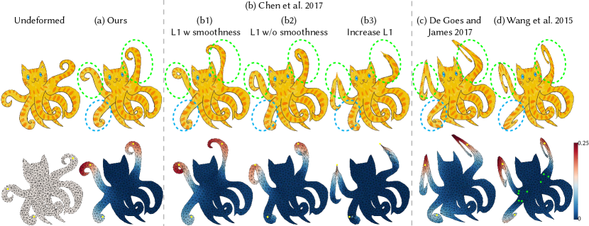
However, direct use of a regularization term leads to artifacts, due to the fact that the -norm competes with the elastic energy by dragging all the vertices towards their original positions. This results in undesired distortion near the deformation handles (see Fig. 3(b) and Fig. 13(b)), making the deformed region look unnatural. Previous -based methods (Chen et al., 2017) focus specifically on ARAP-like deformation, and attempt to alleviate this artifact by adding a Laplacian smoothness term and a weighting term based on biharmonic distance. Unfortunately, as seen in Fig. 3 at the ends of the octocat’s tentacles, artifacts can arise in regions quite close to the deformation handles, and there is not necessarily any setting of these parameters which alleviates these artifacts without oversmoothing the entire deformation.
Inspired by “folded concave” losses in statistical regression (Fan and Li, 2001; Zhang, 2010) and the use of the loss in deformation (Chen et al., 2017), we propose using a smoothly clipped group -norm as our locality-inducing regularization. We call it a SC-L1 loss for “smoothly clamped loss” (see the inset).
We adopt a simple implementation for our SC-L1 loss:
| (1) |
![[Uncaptioned image]](https://cdn.awesomepapers.org/papers/726c1b9e-173f-4053-8262-318cf25291f6/x4.png)
where is the threshold distance beyond which the regularizer is disabled (this is equivalent to a group-variant of the MCP loss in (Zhang, 2010), but we use the term “SC-L1” to emphasize that the minimax concave property is not critical for localized deformation). This function is continuously differentiable and piecewise smooth, and admits a proximal shrinkage operator free of local minima. Near the origin the SC-L1 loss function acts like the group -norm, which drives towards in a sparse-deformation-seeking manner. When , the SC-L1 loss function value is a constant and has no penalty on . For a detailed comparison between our SC-L1 loss function and other alternatives, please see Sec.5 of the supplementary material.
3.2. Local Deformation Energy
We denote as a matrix of vertex positions at the deformed state, and as a matrix containing rest state vertex positions.
The total energy for our local deformation is as follows:
| (2a) | ||||
| (2b) | s.t. | |||
| (2c) | ||||
The first term is an elasticity energy of choice, and can be selected independent of the locality regularization. The second term is the novel “SC-L1 loss” term on the vertex position changes, which measures the locality of the deformation. is the barycentric vertex area of the -th vertex, which ensures the consistency of the result across different mesh resolutions for the same constant . To enable more user control, position constraints and optional affine constraints can be added on selected vertices to achieve different deformation effects. denotes the indices of the vertices with the position constraint, and we call these vertices “handles”. is the -th set of vertex indices where an affine constraint is added. For simplicity, we omit the position constraints and affine constraints in the discussion below, as they can be easily intergrated to the system by removing the corresponding degrees of freedom and using Lagrange multiplier method (see Eq(1) in (Wang et al., 2015)).
Inspired by the local-global strategy in (Brown and Narain, 2021), our local deformation energy (Eq. 2) can be rewritten as:
| (3a) | ||||
| (3b) | s.t. | |||
where is the selection matrix for edges of the -th vertex or element. denotes the symmetric factor computed using the polar decomposition , where is the deformation gradient. Thus is the symmetric factor of deformation gradient of the -th vertex or element. (Note that in general .) The goal of using here is to ensure the local coordinates are invariant to rotations as well as translations. For details, please see (Brown and Narain, 2021).
4. Optimizing With ADMM
A natural way to minimize this energy is to use the alternating direction method of multipliers (Boyd et al., 2011) for the sparsity term, and to use a local-global update strategy for the elasticity term. However, previous -based methods (Chen et al., 2017) apply these two strategies separately in their local and global steps, resulting in an inefficient optimization scheme. As they only support 2D ARAP energy, we discuss further in Sec. 4.1.
We propose a new way to efficiently minimize such energies in Eq. 3 by combining the sparsity-targeted ADMM with the elasticity-focused local-global strategy. We minimize our energy (Eq. 3) using a three-block alternating direction method of multipliers scheme (Boyd et al., 2011) following the local-global update strategy. Our first local step, finding the optimal symmetric factor of the deformation gradient, can be formulated as a minimization problem on its singular values. Our second local step, minimizing the SC-L1 loss term for each , can be solved using a shrinkage step. Our global step, updating vertex positions , is achieved by solving a linear system. We provide an overview of our three-block ADMM scheme in Alg. 1.
4.1. Example I: Local ARAP Energy
We begin by considering how to minimize an as-rigid-as-possible (ARAP) energy (Sorkine and Alexa, 2007) when combined with a SC-L1 loss regularizer. With an ARAP elastic energy, the total energy (Eq. 3) for our local deformation is as follows:
| (4) |
where is a rotation matrix, is a diagonal matrix of cotangent weights, and are matrices of ”spokes and rims” edge vectors of the -th vertex at the rest and deformed states respectively. denotes . Here we use to denote , since we drive the deformation gradient towards a rotation matrix in ARAP energy.
Previous method (Chen et al., 2017) optimizes the version of Eq. 4 in a less efficient way. Their local step optimizes over per-vertex rotation and their global step minimizes over vertex
![[Uncaptioned image]](https://cdn.awesomepapers.org/papers/726c1b9e-173f-4053-8262-318cf25291f6/x5.png)
positions using a two-block ADMM scheme. This leads to an expensive optimization with a full ADMM optimization in each global step, making their method too slow for interactive usage. In contrast, applying our new three-block ADMM scheme to the local ARAP energy results in a much more efficient solver, which is one ADMM optimization itself (see the inset, where the blue regions denote an ADMM optimization). We further show the pseudocode of our three-block ADMM for local ARAP energy in Suppl. Alg.1.
More concretely, by setting , we can further rewrite Eq. 4 as
| (5a) | ||||
| (5b) | s.t. | |||
The above minimization problem can be solved efficiently using the following ADMM update steps:
| (6a) | |||
| (6b) | |||
| (6c) | |||
| (6d) | |||
Here is a fixed penalty parameter. For a detailed derivation of the ADMM update, please see Sec. 2 of the supplementary material.
The various steps in this ADMM-based algorithm are computed as follows:
For updating , local step 1 (Eq. 6a) is an instance of the Orthogonal Procrustes problem, which can be solved in the same way as the rotation fitting step in (Sorkine and Alexa, 2007). The optimal can be computed as from the singular value decomposition of , where .
For updating , following the derivation of the proximal operator of SC-L1 loss in Sec. 1 of the supplementary material, our local step 2 (Eq. 6b) is solved using a SC-L1 loss-specific shrinkage step:
| (7) | |||
| (8) |
To avoid local minima in the shrinkage step, this assumes is set to satisfy (see Sec. 1 of the supplementary material).
For updating , the global step (Eq. 6c) can be achieved by solving a linear system:
| (9) |
where the Laplacian and are defined in the same way as the global step (Eq. 9) in (Sorkine and Alexa, 2007). For fixed an efficient implementation is obtained by precomputing and storing the Cholesky factorization of .
4.2. Example II: Local Neo-Hookean Energy
Our local deformation scheme can be further extended to physics-based elasticity energies, e.g., Neo-Hookean energy. Using the Neo-Hookean energy as our elasticity energy and following the framework of (Brown and Narain, 2021), the optimization problem in Eq. 3 can be written as follows:
| (10a) | ||||
| (10b) | s.t. | |||
where denotes all the elements.
Similarly, by introducing , we can minimize our local Neo-Hookean energy using ADMM. For a detailed derivation, please see Sec. 3 of the supplementary material.
The ADMM update (Alg. 1) for the above minimization problem is as follows:
| (11a) | |||
| (11b) | |||
| (11c) | |||
| (11d) | |||
| (11e) | |||
Here and are fixed penalty parameters.
The local step 2 (updating ) and the global step (updating ) can be solved in the same way as the local ARAP energy (see Sec. 4.1).
For updating , local step 1 (Eq. 11a) can be solved by performing the energy minimization on the singular values of . This is a proximal operator of at the rotation-invariant .
Let us denote the proximal operator of and the singular value decomposition of as:
| (12) | |||
| (13) |
where is the augmented Lagrangian parameter for .
As shown by (Brown and Narain, 2021), we can compute the optimal as:
| (14) | |||
| (15) |
Specifically, one can compute the SVD of and perform the minimization of only on its singular values, while keeping singular vectors unchanged. The above optimization of singular values can be performed using an L-BFGS solver.
4.3. Extension to Other Elastic Energies
Our algorithm can easily generalize across different dimensions and material models. Switching the material model only requires a change on the minimization problem in the local step 1 , which can be optimized over the singular values of the symmetric factor of the deformation gradient.
4.3.1. As-Conformal-As-Possible Energy
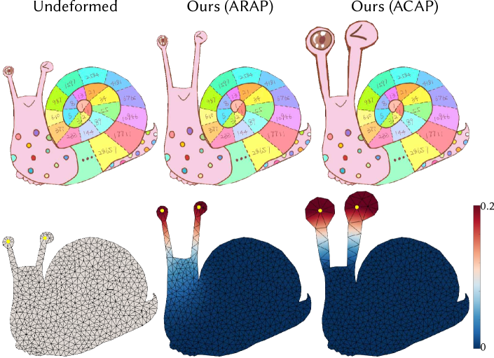
For editing tasks where users intend to locally scale the geometry while preserving the texture, it’s desirable to constrain the angle preservation, or conformality (see Fig. 4 and Fig. 10). We can adapt the ARAP energy to as-conformal-as-possible (ACAP) energy (Bouaziz et al., 2012) by allowing local scaling:
| (16) |
where is a scalar controlling the scaling of the local patch and can be computed analytically (see Sec.4 of the supplementary material).
4.3.2. Cloth
4.3.3. 1D Polyline
Our algorithm can be also extended to the local editing of 1D polyline in vector graphics. The deformation of a polyline can be modeled using the ARAP energy (Eq. 4) with uniform weights.
5. Results
We evaluate our method by comparing it against existing local deformation tools and showcasing its extension to various elastic energies. All the colormaps in our figures visualize the vertex displacement with respect to the rest shape. The accompanying video also includes several animation examples generated using our local deformation tool.
We implement a 2D version of our method in MATLAB with gptoolbox (Jacobson et al., 2018a), and a 3D version in C++ with libigl (Jacobson et al., 2018b) based on the WRAPD framework (Brown and Narain, 2021). We also implement the 2D version of our method in C++ for runtime evaluation and comparison. Benchmarks are performed using a MacBook Pro with an Apple M2 processor and 24GB of RAM for 3D and a Windows desktop with an i9-9900K 3.60 GHz CPU for 2D. Table 2 in the supplementary material shows the performance statistics and relevant parameters of all our examples.
Quality
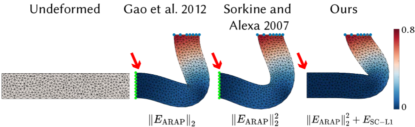
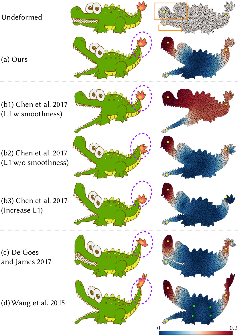
We compare our methods against other local editing tools, including i) -based deformation (Chen et al., 2017), ii) regularized Kelvinlets (De Goes and James, 2017) and iii) biharmonic coordinates (Wang et al., 2015). Among them, the use of -norm regularization (Chen et al., 2017) causes artifacts (see Fig. 3-b and Fig. 13-b). Regularized Kelvinlets technique (De Goes and James, 2017) deforms a shape based on Euclidean distances, thus not shape-aware, creating artifacts when two disjoint parts are close in Euclidean space but far away geodesically (see the blue region in Fig. 3-c and the teeth area in Fig. 13-c). Methods based on biharmonic coordinates, such as (Wang et al., 2015), usually require careful placement of additional fixed control points to pre-determine the ROI. The latter two methods do not minimize any elastic energy in the deformation process, and thus their deformations are more susceptible to shape distortion (see Fig. 13). We additionally compare our method against the sparse deformation method (Gao et al., 2012), which directly introduces a sparsity-induced norm in ARAP energy. As shown in Fig. 2, the resulting deformation is sparse but not local, thus requiring the setup of additional fixed constraints.
In contrast, our method produces the deformation which is local, natural, and shape-aware; it automatically adapts the ROI without the need for careful control primitive setup.
Efficacy
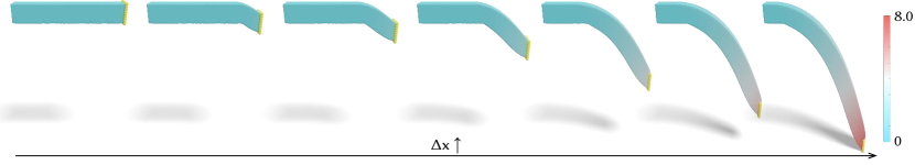
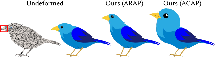
We illustrate the ROI adaptation of our method in different situations: It adapts to different energy models—for example, the local ACAP has a smaller ROI than the local ARAP energy as the former allows for local scaling (see Fig. 4). It also adapts to different extents of deformation. As Fig. 8 demonstrates, the ROI gradually increases as the deformation of the bar becomes larger.
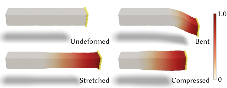
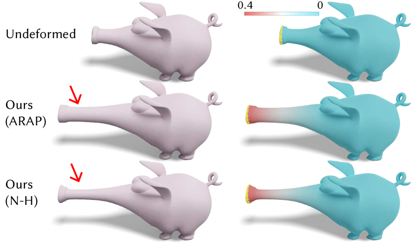
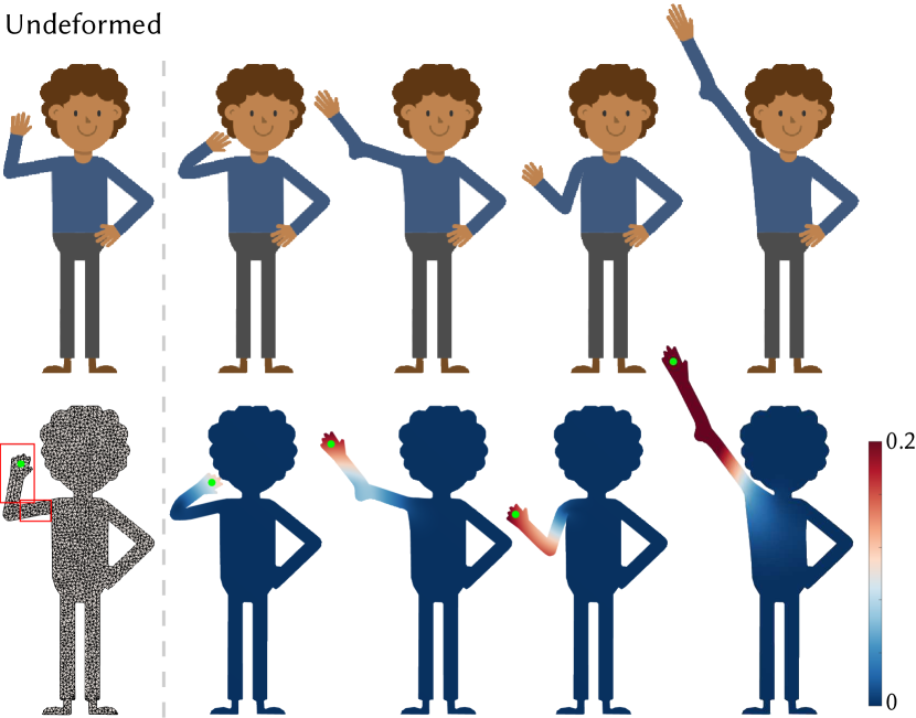
One can configure the local deformation style by choosing various elastic energy models. For example, the local Neo-Hookean energy leads to deformation that preserves volume, while the local ARAP energy is volume agnostic (see Fig. 11). The deformation can be further tuned by introducing additional affine constraints—for instance, to enable the character to wave hands (Fig. 12) or the crocodile to open its mouth (Fig. 13)—in a natural way.
Performance
In terms of performance, our solver is able to efficiently minimize the energy at interactive rate, while the method of (Chen et al., 2017) is too slow to run in realtime. Because their method only supports 2D ARAP energy, in Table 1 of the supplementary material, we evaluate the runtime of our method (using both the SC-L1 loss and loss) and (Chen et al., 2017) on a 2D ARAP local energy and across different mesh resolutions and deformations. Measured with the same convergence threshold, our method runs orders of magnitude faster than (Chen et al., 2017), achieving roughly speedup for small deformation and speedup for large deformation.
Extensibility
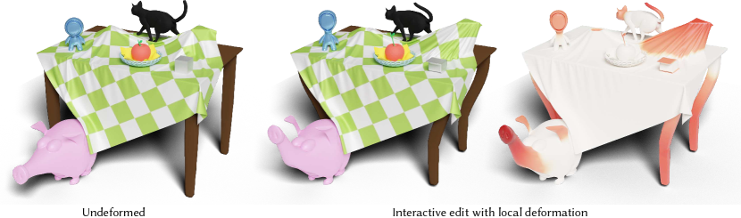
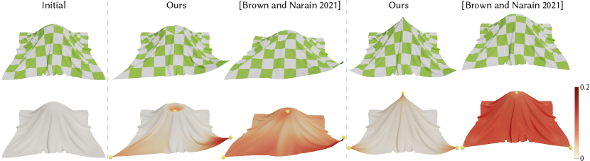
Our method can easily generalize to other dimensions and material models, such as the ACAP deformation, cloth deformation, and 1D polyline deformation (see Fig. 10 and Fig. 4). The local ACAP energy enables local scaling and better preserves the texture around the deformed region. In Fig. 7, the user can interactively edit a polyline and naturally recovers its rest shape, which is a desirable feature by the users. In Fig. 6, to deform a cloth in a physically plausible way, the deformation locality is particularly useful, as otherwise a local edit of the cloth may cause a global change leading to unexpected intersections with other objects. Lastly, to demonstrate our method in a more complex scenario, an editing session involving multiple objects and clothes is shown in Fig. 1.
6. CONCLUSION & FUTURE WORK
We describe a regularization based on an “SC-L1 loss” which provides an effective and simple to implement tool for localizing an elastic energy driven deformation to only those regions of a shape being manipulated by a user. The region of influence induced by our method naturally adapts to the geometry of the shape, the size of the deformation, and the elastic energy being used. Furthermore SC-L1 regularization is generic enough to be applied to a wide range of shapes and elastic energies, including 1D, 2D, 3D and cloth finite element deformation, and is fast enough to be used in real-time. Our proposed approach offers several benefits for shape manipulation: It avoids undesired movement in far-off regions of a shape when only one part is being moved by the user, it allows parts of a shape to be deformed with direct manipulation without a pre-rigging step, and avoids the visual artifacts of previous work.
There remain several issues related to localized shape deformation not addressed by our method. Firstly our regularization is applied independently per-vertex, which makes it difficult to apply to splines, NURBS, or even meshes with highly irregular element sizes, which we mark an important direction for future work. In addition, since we use an ADMM method in the optimization, our approach suffers from the common shortcomings of applying ADMM to non-convex energies, including lack of convergence guarantees and slow convergence when high precision is required. Exploration of other optimization algorithms alleviating these issues is another useful future direction. Finally, although it is out of scope for our work here, we note in particular the usefulness of incorporating localized elastic energy deformation into sculpting workflows for artists. This involves a number of facets: Choosing the correct elastic energy to achieve an artistic effect, providing an intuitive UI to adjust the scale of the ROI (for instance by adjusting and , see Fig. 9 and the supplementary video), and in ensuring that our tool integrates well with other sculpting tools. This is particularly useful when handling large “freeform” deformations, as the elastic energy will tend to fight against such deformations, making other tools more suitable. One simple idea for this is to simply reset the rest shape after each click-and-drag, since each deformation step is then independent of the others, and one could switch between our method and others at each step. We have found this mode of interaction to be useful even when only using our method, as it leads to a simple sculpting-style interface, and we include some examples in the supplementary video.
Acknowledgements.
This work is funded in part by National Science Foundation (1910839). We especially thank George E. Brown for sharing the WRAPD implementation and the help with setting up experiments. We thank Jiayi Eris Zhang and Danny Kaufman for sharing the undeformed scene geometry; Lillie Kittredge and Huy Ha for proofreading; Rundi Wu for the help with rendering; all the artists for sharing the 2D and 3D models and anonymous reviewers for their helpful comments and suggestions.References
- (1)
- Alexa (2006) Marc Alexa. 2006. Mesh Editing Based on Discrete Laplace and Poisson Models. In ACM SIGGRAPH 2006 Courses (Boston, Massachusetts) (SIGGRAPH ’06). Association for Computing Machinery, New York, NY, USA, 51–59.
- Ben-Chen et al. (2009) Mirela Ben-Chen, Ofir Weber, and Craig Gotsman. 2009. Variational Harmonic Maps for Space Deformation. ACM Trans. Graph. 28, 3, Article 34 (Jul 2009), 11 pages.
- Bergou et al. (2006) Miklos Bergou, Max Wardetzky, David Harmon, Denis Zorin, and Eitan Grinspun. 2006. A Quadratic Bending Model for Inextensible Surfaces. In Proceedings of the Fourth Eurographics Symposium on Geometry Processing (Cagliari, Sardinia, Italy) (SGP ’06). Eurographics Association, Goslar, DEU, 227–230.
- Bertsekas (1996) D.P. Bertsekas. 1996. Constrained Optimization and Lagrange Multiplier Methods. Athena Scientific, Nashua.
- Bouaziz et al. (2012) Sofien Bouaziz, Mario Deuss, Yuliy Schwartzburg, Thibaut Weise, and Mark Pauly. 2012. Shape-Up: Shaping Discrete Geometry with Projections. Comput. Graph. Forum 31, 5 (Aug 2012), 1657–1667.
- Boyd et al. (2011) Stephen Boyd, Neal Parikh, Eric Chu, Borja Peleato, and Jonathan Eckstein. 2011. Distributed Optimization and Statistical Learning via the Alternating Direction Method of Multipliers. Found. Trends Mach. Learn. 3, 1 (Jan 2011), 1–122.
- Brandt and Hildebrandt (2017) Christopher Brandt and Klaus Hildebrandt. 2017. Compressed vibration modes of elastic bodies. Computer Aided Geometric Design 52-53 (2017), 297–312. Geometric Modeling and Processing 2017.
- Brown and Narain (2021) George E. Brown and Rahul Narain. 2021. WRAPD: Weighted Rotation-aware ADMM for Parameterization and Deformation. ACM Transactions on Graphics (Proc. SIGGRAPH) 40, 4 (8 2021).
- Cani and Angelidis (2006) Marie-Paule Cani and Alexis Angelidis. 2006. Towards Virtual Clay. In ACM SIGGRAPH 2006 Courses (Boston, Massachusetts) (SIGGRAPH ’06). Association for Computing Machinery, New York, NY, USA, 67–83. https://doi.org/10.1145/1185657.1185676
- Chen and Desbrun (2022) Jiong Chen and Mathieu Desbrun. 2022. Go Green: General Regularized Green’s Functions for Elasticity. In ACM SIGGRAPH 2022 Conference Proceedings (Vancouver, BC, Canada) (SIGGRAPH ’22). Association for Computing Machinery, New York, NY, USA, Article 6, 8 pages.
- Chen et al. (2017) Jiaxu Chen, Long Zhang, Xiaoxu Li, Bo Zhang, and Zhongfu Ye. 2017. Locally controlled as-rigid-as-possible deformation for 2D characters. Computer Animation and Virtual Worlds 28, 6 (2017), e1750. e1750 cav.1750.
- Coquillart (1990) Sabine Coquillart. 1990. Extended Free-Form Deformation: A Sculpturing Tool for 3D Geometric Modeling. SIGGRAPH Comput. Graph. 24, 4 (Sep 1990), 187–196.
- De Goes and James (2017) Fernando De Goes and Doug L. James. 2017. Regularized Kelvinlets: Sculpting Brushes Based on Fundamental Solutions of Elasticity. ACM Trans. Graph. 36, 4, Article 40 (Jul 2017), 11 pages.
- De Goes and James (2018) Fernando De Goes and Doug L. James. 2018. Dynamic Kelvinlets: Secondary Motions Based on Fundamental Solutions of Elastodynamics. ACM Trans. Graph. 37, 4, Article 81 (Jul 2018), 10 pages.
- de Goes and James (2019) Fernando de Goes and Doug L. James. 2019. Sharp Kelvinlets: Elastic Deformations with Cusps and Localized Falloffs. In Proceedings of the 2019 Digital Production Symposium (Los Angeles, California) (DigiPro ’19). Association for Computing Machinery, New York, NY, USA, Article 2, 8 pages.
- Deng et al. (2013) Bailin Deng, Sofien Bouaziz, Mario Deuss, Juyong Zhang, Yuliy Schwartzburg, and Mark Pauly. 2013. Exploring Local Modifications for Constrained Meshes. Computer Graphics Forum 32, 2pt1 (2013), 11–20.
- Fan and Li (2001) Jianqing Fan and Runze Li. 2001. Variable Selection via Nonconcave Penalized Likelihood and its Oracle Properties. J. Amer. Statist. Assoc. 96, 456 (2001), 1348–1360.
- Gao et al. (2012) Lin Gao, Guoxin Zhang, and Yu-Kun Lai. 2012. Lp shape deformation. Science China Information Sciences 55 (05 2012).
- Genova et al. (2020) Kyle Genova, Forrester Cole, Avneesh Sud, Aaron Sarna, and Thomas Funkhouser. 2020. Local Deep Implicit Functions for 3D Shape. In Proceedings of the IEEE/CVF Conference on Computer Vision and Pattern Recognition. 4857–4866.
- Hahn et al. (2012) Fabian Hahn, Sebastian Martin, Bernhard Thomaszewski, Robert Sumner, Stelian Coros, and Markus Gross. 2012. Rig-Space Physics. ACM Trans. Graph. 31, 4, Article 72 (Jul 2012), 8 pages.
- Hoschek et al. (1993) Josef Hoschek, Dieter Lasser, and Larry L. Schumaker. 1993. Fundamentals of Computer Aided Geometric Design. A. K. Peters, Ltd., USA.
- Jacobson et al. (2018a) Alec Jacobson et al. 2018a. gptoolbox: Geometry Processing Toolbox. http://github.com/alecjacobson/gptoolbox.
- Jacobson et al. (2012) Alec Jacobson, Ilya Baran, Ladislav Kavan, Jovan Popović, and Olga Sorkine. 2012. Fast Automatic Skinning Transformations. ACM Trans. Graph. 31, 4, Article 77 (Jul 2012), 10 pages.
- Jacobson et al. (2011) Alec Jacobson, Ilya Baran, Jovan Popović, and Olga Sorkine. 2011. Bounded Biharmonic Weights for Real-Time Deformation. ACM Trans. Graph. 30, 4, Article 78 (Jul 2011), 8 pages.
- Jacobson et al. (2018b) Alec Jacobson, Daniele Panozzo, et al. 2018b. libigl: A simple C++ geometry processing library. https://libigl.github.io/.
- Joshi et al. (2007) Pushkar Joshi, Mark Meyer, Tony DeRose, Brian Green, and Tom Sanocki. 2007. Harmonic Coordinates for Character Articulation. ACM Trans. Graph. 26, 3 (Jul 2007), 71–es.
- Kavan and Sorkine (2012) Ladislav Kavan and Olga Sorkine. 2012. Elasticity-Inspired Deformers for Character Articulation. ACM Trans. Graph. 31, 6, Article 196 (Nov 2012), 8 pages.
- Kho and Garland (2005) Youngihn Kho and Michael Garland. 2005. Sketching Mesh Deformations. ACM Trans. Graph. 24, 3 (Jul 2005), 934.
- Lipman et al. (2008) Yaron Lipman, David Levin, and Daniel Cohen-Or. 2008. Green Coordinates. ACM Trans. Graph. 27, 3 (Aug 2008), 1–10.
- Luo et al. (2007) Qiong Luo, Bo Liu, Zhan-Guo Ma, and Hong-Bin Zhang. 2007. Mesh Editing in ROI with Dual Laplacian. In Computer Graphics, Imaging and Visualisation (CGIV 2007). 195–199. https://doi.org/10.1109/CGIV.2007.57
- Magnenat-Thalmann et al. (1989) N. Magnenat-Thalmann, R. Laperrière, and D. Thalmann. 1989. Joint-Dependent Local Deformations for Hand Animation and Object Grasping. In Proceedings on Graphics Interface ’88 (Edmonton, Alberta, Canada). Canadian Information Processing Society, CAN, 26–33.
- Mohimani et al. (2007) G. Hosein Mohimani, Massoud Babaie-Zadeh, and Christian Jutten. 2007. Fast Sparse Representation Based on Smoothed l0 Norm. In Independent Component Analysis and Signal Separation. Springer Berlin Heidelberg, Berlin, Heidelberg, 389–396.
- Neumann et al. (2013) Thomas Neumann, Kiran Varanasi, Stephan Wenger, Markus Wacker, Marcus Magnor, and Christian Theobalt. 2013. Sparse Localized Deformation Components. ACM Trans. Graph. 32, 6, Article 179 (Nov 2013), 10 pages.
- Peng et al. (2018) Yue Peng, Bailin Deng, Juyong Zhang, Fanyu Geng, Wenjie Qin, and Ligang Liu. 2018. Anderson Acceleration for Geometry Optimization and Physics Simulation. ACM Trans. Graph. 37, 4, Article 42 (Jul 2018), 14 pages. https://doi.org/10.1145/3197517.3201290
- Poranne et al. (2017) Roi Poranne, Marco Tarini, Sandro Huber, Daniele Panozzo, and Olga Sorkine-Hornung. 2017. Autocuts: Simultaneous Distortion and Cut Optimization for UV Mapping. ACM Transactions on Graphics (proceedings of ACM SIGGRAPH ASIA) 36, 6 (2017).
- Sederberg and Parry (1986) Thomas W. Sederberg and Scott R. Parry. 1986. Free-Form Deformation of Solid Geometric Models. In Proceedings of the 13th Annual Conference on Computer Graphics and Interactive Techniques (SIGGRAPH ’86). Association for Computing Machinery, New York, NY, USA, 151–160.
- Shtengel et al. (2017) Anna Shtengel, Roi Poranne, Olga Sorkine-Hornung, Shahar Z. Kovalsky, and Yaron Lipman. 2017. Geometric Optimization via Composite Majorization. ACM Trans. Graph. 36, 4, Article 38 (jul 2017), 11 pages. https://doi.org/10.1145/3072959.3073618
- Singh and Fiume (1998) Karan Singh and Eugene Fiume. 1998. Wires: A Geometric Deformation Technique. In Proceedings of the 25th Annual Conference on Computer Graphics and Interactive Techniques (SIGGRAPH ’98). Association for Computing Machinery, New York, NY, USA, 405–414.
- Smith et al. (2019) Breannan Smith, Fernando De Goes, and Theodore Kim. 2019. Analytic Eigensystems for Isotropic Distortion Energies. ACM Trans. Graph. 38, 1, Article 3 (Feb 2019), 15 pages. https://doi.org/10.1145/3241041
- Sorkine and Alexa (2007) Olga Sorkine and Marc Alexa. 2007. As-Rigid-as-Possible Surface Modeling. In Proceedings of the Fifth Eurographics Symposium on Geometry Processing (Barcelona, Spain) (SGP ’07). Eurographics Association, Goslar, DEU, 109–116.
- Wang et al. (2015) Yu Wang, Alec Jacobson, Jernej Barbič, and Ladislav Kavan. 2015. Linear Subspace Design for Real-Time Shape Deformation. ACM Trans. Graph. 34, 4, Article 57 (Jul 2015), 11 pages. https://doi.org/10.1145/2766952
- Xiang et al. (2022) Jianhong Xiang, Hao Xiang, Linyu Wang, and Yu Zhong. 2022. Medical Image Reconstruction Method Based on Smooth L0 Norm. https://doi.org/10.21203/rs.3.rs-1535219/v1
- Xu et al. (2015) Linlin Xu, Ruimin Wang, Juyong Zhang, Zhouwang Yang, Jiansong Deng, Falai Chen, and Ligang Liu. 2015. Survey on sparsity in geometric modeling and processing. Graphical Models 82 (2015), 160–180.
- Zhang (2010) Cun-Hui Zhang. 2010. Nearly unbiased variable selection under minimax concave penalty. The Annals of Statistics 38, 2 (2010), 894 – 942. https://doi.org/10.1214/09-AOS729
- Zhang et al. (2019) Juyong Zhang, Yue Peng, Wenqing Ouyang, and Bailin Deng. 2019. Accelerating ADMM for Efficient Simulation and Optimization. ACM Trans. Graph. 38, 6, Article 163 (nov 2019), 21 pages. https://doi.org/10.1145/3355089.3356491
- Zhang et al. (2022) Jiayi Eris Zhang, Jèrèmie Dumas, Yun (Raymond) Fei, Alec Jacobson, Doug L. James, and Danny M. Kaufman. 2022. Progressive Simulation for Cloth Quasistatics. ACM Trans. Graph. 41, 6, Article 218 (2022).
- Zhu et al. (2018) Yufeng Zhu, Robert Bridson, and Danny M. Kaufman. 2018. Blended Cured Quasi-Newton for Distortion Optimization. ACM Trans. on Graphics (2018).
- Zimmermann et al. (2007) Johannes Zimmermann, Andrew Nealen, and Marc Alexa. 2007. SilSketch: Automated Sketch-Based Editing of Surface Meshes. In EUROGRAPHICS Workshop on Sketch-Based Interfaces and Modeling, Michiel van de Panne and Eric Saund (Eds.). The Eurographics Association. https://doi.org/10.2312/SBM/SBM07/023-030


Black Man Waving Hand Cartoon Vector.svg from Wikimedia Commons by Videoplasty.com, CC-BY-SA 4.0.
See pages - of figures/supplementary.pdf