¹¹institutetext: Ben-Gurion University of the Negev, Israel
¹¹email: {dinitz, dolev}@cs.bgu.ac.il, [email protected]

Local Deal-Agreement Based Monotonic
Distributed Algorithms for Load Balancing
in General Graphs
(Preliminary Version)

Yefim Dinitz 11 Shlomi Dolev 11 Manish Kumar 11

Abstract

In computer networks, participants may cooperate in processing tasks, so that loads are balanced among them. We present local distributed algorithms that (repeatedly) use local imbalance criteria to transfer loads concurrently across the participants of the system, iterating until all loads are balanced. Our algorithms are based on a short local deal-agreement communication of proposal/deal, based on the neighborhood loads. They converge monotonically, always providing a better state as the execution progresses. Besides, our algorithms avoid making loads temporarily negative. Thus, they may be considered anytime ones, in the sense that they can be stopped at any time during the execution. We show that our synchronous load balancing algorithms achieve $\epsilon$ -Balanced state for the continuous setting and 1-Balanced state for the discrete setting in all graphs, within $O(nD\log(nK/\epsilon))$ and $O(nD\log(nK/D)+nD^{2})$ time, respectively, where $n$ is the number of nodes, $K$ is the initial discrepancy, $D$ is the graph diameter, and $\epsilon$ is the final discrepancy. Our other monotonic synchronous and asynchronous algorithms for the discrete setting are generalizations of the first presented algorithms, where load balancing is performed concurrently with more than one neighbor. These algorithms arrive at a 1-Balanced state in time $O(nK^{2})$ in general graphs, but have a potential to be faster as the loads are balanced among all neighbors, rather than with only one; we describe a scenario that demonstrates the potential for a fast ( $O(1)$ ) convergence. Our asynchronous algorithm avoids the need to wait for the slowest participants’ activity prior to making the next load balancing steps as synchronous settings restrict. We also introduce a self-stabilizing version of our asynchronous algorithm.

Keywords:

Distributed algorithms Deterministic Load balancing Self-Stabilization Monotonic

1 Introduction

The load balancing problem is defined when there is an undirected network (graph) of computers (nodes), each one assigned a non-negative working load, and they like to balance their loads. If nodes $u$ and $v$ are connected by an edge in the graph, then any part of the load of $u$ may be transferred over that edge from $u$ to $v$ , and similarly from $v$ to $u$ . The possibility of balancing loads among computers is a fundamental benefit of the possible collaboration and coordination in distributed systems. The application and scope change over time, for example, the scopes include grid computing, clusters, and clouds.

We assume that computation in the distributed systems is concurrent, that is, at any node, the only way to get information on the graph is by communicating with its neighbors. The initial information at a node is its load and the list of edges connecting it to its neighbors. The ideal goal of load balancing to make all nodes load equal to the average load; usually, some approximation to the ideal balancing is looked for, in order to avoid global operations (such as a preprocessed leader election based load balancing, where a leader node should be able to collect, while the system waits, store and process information from the entire system). An accepted global measure for the deviation of a current state from the balanced one is its (global) discrepancy, defined as $K=L_{max}-L_{min}$ , where $L_{max}$ , resp., $L_{min}$ , is the currently maximum, resp., minimum, node load in the graph. An alternative way to measure the deviation is in terms of local imbalance which is the maximal difference of loads between neighboring nodes. A state is said to be $\epsilon$ -Balanced if that maximal local difference is at most $\epsilon$ (e.g., “locally optimal load balancing” in [15] is a 1-Balanced state in our terms). The continuous and discrete (integer) versions of the problem are distinguished. In the continuous setting, any amount of the load may be transferred over edges, while at the discrete setting, all loads and thus also all transfer amounts should be integers. In this paper, we concentrate on deterministic algorithms solving the problem in a time polynomial in the global input size, that is in the number $n$ of graph nodes and in the logarithm of the maximal load.

The research on the load balancing problem has a long history. The two pioneering papers solving the problem are those of Cybenko [8] and Boillat [7]. Both are based on the concept of diffusion: at any synchronized round, every node divides a certain part of its load equally among its neighbors, keeping the rest of its load for itself; for regular graphs, the load fraction kept for itself is usually set to be equal to that sent to each neighbor. Many further solutions are based on diffusion, see [23, 6, 2, 5, 1, 19]. Most of the papers consider $d$ -regular graphs, and use Markov chains and ergodic theory for deriving the rate of convergence. This approach works smoothly in the continuous setting.

Diffusion methods in the discrete setting requires rounding of every transferred amount, which makes the analysis harder; Rabani et al. [23] made substantial advancement in that direction. However, the final discrepancy achieved by their method is not constant. As mentioned in [14], the discrepancy cannot be reduced below $\Omega(d_{min}\cdot D)$ by a deterministic diffusion-based algorithm, where $D$ is the diameter of the graph and $d_{min}$ is the minimum degree in the graph. The algorithms in papers [13, 14] are based on randomized post-processing, using random walks, for decreasing the discrepancy to a constant with high probability.

One of the alternatives to diffusion is the matching approach. There, a node matching is chosen at the beginning of each synchronized round, and after that every two matched nodes balance their loads. See, e.g., [18, 24]. In known deterministic algorithms, those matching, are usually chosen in advance according to the graph structure; in randomized algorithms, they are chosen randomly. The deterministic matching algorithms of Feuilloley et al. [15] achieve a 1-Balanced final state for general graphs, in time not depending on the graph size $n$ and depending cubically, and also exponentially for the discrete setting, on the initial discrepancy $K$ . These algorithms extensively use communication between nodes. (In the further discussion, we do not relate to the approach and results of Feuilloley et al. [15], since the used computational model is different from that we concentrate on.) Yet another balancing circuits [3, 23] approach is based on sorting circuits [23], where each 2-input comparator balances the loads of its input nodes (instead of the comparison), see e.g., [4]. Randomized matching and balancing circuits algorithms of [24] achieve a constant final discrepancy w.h.p.

All the above-mentioned papers use the synchronous distributed model. The research on load balancing in the asynchronous distributed setting (where the time of message delivery is not constant and might be unpredictably large) is not extensive. The only theoretically based approach suggested for it is turning the asynchronous setting into synchronous by appropriately enlarging the time unit, see e.g., [1].

Note that the suggested solutions ignore the possibility of a short coordinating between nodes. A node just informs each of its neighbor on the load amount transferred to it, if any, and lets the neighbors know on its own resulting load after each round. In previous diffusion based load balancing works, only its own load and the pre-given distribution policy define the decisions at each node; as a maximum, a node also pays attention to the current loads at its neighbors.

The above-mentioned approaches leave the following gaps in the suggested solutions (among others):

•

Following [9, 21], we call an algorithm anytime, if any of its intermediate solutions is feasible and not worse than the previous ones; thus, it may be used immediately in the case of a need/emergency. In particular, this property of algorithms is important for the message-passing settings where the actual time of message delivery might be long. In the suggested solutions to the load balancing problem, to the contrast, either, loads might become negative (see, e.g, [14, 17, 24, 2]), which is not appropriate in an output, or the discrepancy might grow w.r.t. previous states (see, e.g, [23, 24]).
•

The general graph case is more or less neglected in the literature; instead, most of the papers focus on $d$ -regular graphs. There are only a few brief remarks on the possibility of generalizing the results to general graphs, see, e.g., [23, second paragraph].
•

The final discrepancy achieved by the deterministic algorithms is far not a constant.
•

The asynchronous setting is explored quite weakly in the literature. There, no worst-case bounds for achieving the (almost) balanced state are provided.

We suggest using the distributed computing approach in load balancing, based on short agreement between neighboring nodes. By our algorithms, we tried to close the gaps as above, as far as possible. In this paper, we concentrate on deterministic algorithms with deterministic worst-case analysis, leaving the development of randomized algorithms (that fit scenarios in which no hard deadlines are required) for further research.

We develop local distributed algorithms, in the sense that each node uses the information on its neighborhood only, with no global information collected at the nodes. The advantage to this is that there is no “entrance fee”, so that the actual running time of an algorithm can be quite small, if we are lucky, say, if we have a starting imbalance that can be balanced in small areas without influencing the entire system; in Section 3, we describe a scenario, which demonstrates the potential for a fast convergence. Accordingly, we choose the ideal goal of a discrete local algorithm to be a $1$ -Balanced state, rather than a small discrepancy. Indeed, let us consider a graph that is a path of length $2n-1$ , where the node loads are 0, 1, 1, 2, 2, …, $n-1$ , $n-1$ , $n$ , along it. No node has a possibility to improve the load balancing in its neighborhood, while the discrepancy is $n$ , a half of the number of graph nodes.

We say that a load balancing algorithm is monotonic if the following conditions always hold during any its execution: (a) each load transfer is from a higher loaded node to a less loaded one, and (b) the maximal load value never increases and the minimal load value never decreases. By item (b), the discrepancy never increases during any execution of a monotonic algorithm, and negative loads are never created, that is, any monotonic algorithm is anytime.

Our main results are as follows, where $D$ is the graph diameter, and $\epsilon$ is the an arbitrarily small bound for the final discrepancy bound. We call an algorithm a single proposal one, if each node at each round proposes a load transfer to at most one node and accepts a proposal of at most one node, and a distributed proposal one, when proposals can be made/accepted to/from several nodes.

•

In the continuous setting, the first synchronized deterministic algorithm for general graphs, which is monotonic and works in time $O(nD\log(nK/\epsilon))$ .
•

In the discrete setting, the first deterministic algorithms for general graphs achieving a 1-Balanced state in time depending on the initial discrepancy logarithmically. It is monotonic and works in time $O(nD\log(nK/D)+nD^{2})$ .
•

Distributed proposals scheme that generalizes the single proposal scheme of those two algorithms.
•

First asynchronous anytime load balancing algorithm.
•

A self-stabilizing version of our asynchronous algorithm.

Remark: Let us consider the place of single proposal algorithms in the classification of load balancing algorithms. At each round, each node $u$ participates in at most two load transfers: one where it transfers a load and one where it receives a load. In other words, the set of edges with transfers, each oriented in the transfer direction, forms a kind of matching, where both in- and out-degree of any node are at most 1 each. This property may be considered a generalization of the matching approach to load balancing. Therefore, one may call single proposal algorithms “short agreement based generalized matching” ones.

Let us compare the results achieved by our two single proposal algorithms with those achieved by deterministic algorithms in Rabani et al. [23]. As of the scope of [23], details are provided there for the $d$ -regular graphs only, and there is no anytime property. For continuous setting, consider the time bound $O\left(\frac{\ln(Kn^{2}/\epsilon)}{(1-\lambda)}\right)$ of [23] for reaching the discrepancy of $\epsilon$ in the worst case. It is the same as our bound in its logarithmic part. Its factor of $\frac{1}{1-\lambda}$ is $\Theta(n^{2})$ in the worst case, e.g., for a graph that is a cycle. Also, the factor $nD$ in our bound is $\Theta(n^{2})$ in the worst case. We conclude that the worst-case bounds overall graphs of the same size are both $O(n^{2}\log(Kn))$ . Note that the class of instances bad for the time bound $O\left(\frac{\log(Kn)}{1-\lambda}\right)$ is quite wide. Consider an arbitrary graph $G$ and add to it a cycle of length $n$ with a single node common with $G$ . We believe that the time bound for the resulting graph will not be better than for a cycle of length $n$ , that is $O(n^{2}\log(Kn))$ . For the discrete setting, we achieve a 1-Balanced state, which is not achieved in Rabani et al. [23]. As on discrepancy (which is our secondary goal), we guarantee discrepancy $D$ , while the final discrepancy in [23] is $O\left(\frac{d\log n}{1-\lambda}\right)$ ; we believe that in the class of instances as described above but with the added cycle of length $D$ , the latter bound is $O(dD^{2}\log(n))$ .

Summarizing, the main contribution of this paper to the load balancing research is turning attention of the load balancing community: (a) to using standard distributed computing methods, that is to short agreement based local distributed algorithms, (b) to the general graphs case, and (c) to anytime monotonic algorithms, and making first steps in these three directions.

Organization of the paper. Section 1.2 presents a summary of related work. The two single proposal algorithms are presented in Section 2, with the analysis. Section 3 describes and analyzes the distributed proposal algorithms. Section 4 discusses the asynchronous version of load balancing algorithms. Section 5 introduces a self-stabilizing version of our asynchronous algorithm. The conclusion appears in Section 6.

1.1 Diffusion vs Deal-Agreement based Load balancing Algorithms

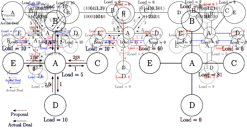
To gain intuition we start with an example. Consider Fig. 1, each node is transferring the load to its neighbor but in the next iteration node $A$ has a large load, which may lead to more iterations of the algorithm for balancing the load. Note that the original load, 5, becomes 21 following the load diffusion. In each round of deal-agreement based load balancing algorithm, each node computes the deal (amount of load accepted by a node without violating the value of TentativeLoad) individually then transfers the load to its neighbors. An example of our deal-agreement based load balancing appears in Fig. 2, node $A$ receives the load from the neighbors according to the proposal up to the value of TentativeLoad but never exceeds the TentativeLoad (load of the node after giving loads to its neighbors). Note that the loads are transferring towards 1-Balanced without violating the condition of monotonicity. Our deal-agreement based algorithm is an anytime and monotonic algorithm that ensures the maximal load bound of nodes is not exceeded. Namely, if there is an upper bound on the loads that can be accumulated in a single node, then starting with loads that respect this bound the bound is not violated due to load exchanges. As opposite to diffusion based algorithms, e.g., load value 21 on node A in Fig. 1 may exceed the capacity of a node.

Refer to caption — Figure 1: Example of Diffusion Load Balancing Algorithm

1.2 Related Work

In this section, we review some related results for load balancing dealing with diffusion, matching, and random-walk based algorithms only.

•

Continuous Diffusion. Continuous load balancing is an “ideal” case (continuous case of Rabani et al. [23]) where the load can be divided arbitrarily. Therefore, it is possible to balance the load perfectly. Muthukrishnan et al. [20] refers the above continuous diffusion model discussed in Rabani et al. [23], as the first order scheme and extend to second order scheme which take $O(\log(Kn))/(1-\lambda))$ time for achieving discrepancy of $O(dn/(1-\lambda))$ , where $\lambda$ is the second largest eigenvalue of diffusion matrix, $K$ is initial discrepancy and $n$ is number of node in the graph. Further progress was made by Rabani et al. [23] who introduced the so-called local divergence, which is an effective way to compute the deviation between actual load and deviation generated by a Markov chain. They proved that the local divergence yields bound on the maximum deviation between the continuous and discrete case for both the diffusion and matching model. They proved that local divergence can be reduced to $O(d\log(Kn)/(1-\lambda))$ in $O(\log(Kn))/(1-\lambda))$ rounds for a d-regular graph.
•

Discrete Diffusion. In discrete load balancing only non-divisible loads are allowed to transfer. In this case, the graph can not be completely balanced. Akbari et al. [2] discussed a randomized and discrete load balancing algorithm for general graph that balances the load up to a discrepancy of $O(\sqrt{d\log n})$ in $O(\log(Kn)/(1-\lambda))$ time, where $d$ in maximum degree, $K$ is the initial discrepancy, and $\lambda$ is the second-largest eigenvalue of the diffusion matrix. Using the algorithm of Akbari et al. [2], discrepancy reduces for other topology also. Such as, for hypercubes, discrepancy reduces to $O(\log n)$ and for expanders and torus graph reduces to $O(\sqrt{\log n})$ .

Randomized diffusion based algorithms [5, 2, 17] are algorithms in which every node distributes its load as evenly as possible among its neighbors and itself. If the remaining load is not possible to distribute without dividing some load then the node redistributes the remaining loads to its neighbors randomly. In Berenbrink et al. [5] authors show randomized diffusion based discrete load balancing algorithm for which discrepancy depends on the expansion property of the graph (e.g., $\lambda$ which is the second-largest eigenvalue of the diffusion matrix and $d$ maximum degree of any node in the graph). Other Quasi-random diffusion based algorithm for general graph [17] considered bounded-error property, where sum of rounding errors on each edge is bounded by some constant time at all time. The discrepancy results of the randomized algorithms in [5, 17] are further improved to $O(d^{2}\sqrt{\log n})$ and $O(d\sqrt{\log n})$ respectively by applying the results from [24], where tighter bounds are obtained for certain graph parameters used in discrepancy bounds of [5, 17].

One of the alternatives to diffusion is the matching approach, also known as the dimension exchange model. In this model for each step, an arbitrary matching of nodes is given, and two matched nodes balance their loads. Friedrich et al. [18] considered a dimension exchange algorithm for the matching model. There every node which is connected to a matching edge computes the load difference over that edge. If the load difference is positive, the load moves between the nodes of that edge. This work reduces the discrepancy to $O\left(\sqrt{\log^{3}n/(1-\lambda)}\right)$ in $O(\log(Kn)/(1-\lambda))$ steps with high probability for general graph. This result [18] is improved by Sauerwald et al. [24] where they achieve constant discrepancy in $O(\log(Kn)/(1-\lambda))$ steps with high probability for regular graph in the random matching model. The constant is independent of the graph and the discrepancy $K$ . The random matching model is an alternative model of balancing circuit, where random matching generated in each round. Additionally, the deterministic matching algorithm of [15] achieves a constant final discrepancy of $O((\log n)^{\epsilon})$ for an arbitrarily small constant $\epsilon>0$ , but after a large number of rounds, depending cubically on the initial discrepancy where $K\geq n$ .

Table 1: Comparison of different Load Balancing algorithms for the general graph (where $n$ is the number of nodes, $d$ is the maximum degree of a node, $K$ is the initial discrepancy, $D$ is the graph diameter, $\lambda$ is the second highest eigenvalue of the diffusion matrix, $\alpha$ is the edge expansion value of the graph, $\epsilon>0$ is an arbitrarily small constant, D’ represent Deterministic algorithm, R’ represent Randomized algorithm, I represent Discrete(Integer), C represent Continuous)

Algorithms	Type	Approach	Transfer	Final discrepancy	Rounds	Anytime
(References)		(Diffusion/	(I/C)	( $L_{max}-L_{min}$ )	(Steps)
		Matching)
Synchronous Model
Rabani et al. [23]	D’	Diffusion/Matching	I	$O\left(\frac{d\log n}{1-\lambda}\right)$	$O\left(\frac{\log(Kn)}{1-\lambda}\right)$	No
			C	$\epsilon$	$O\left(\frac{\ln(Kn^{2}/\epsilon)}{(1-\lambda)}\right)$	No
Muthukrishnan	D’	Diffusion	C	$O\left(\frac{dn}{1-\lambda}\right)$	$O\left(\frac{\log(Kn)}{1-\lambda}\right)$	No
et al. [20]
Akbari et al. [2]	R’	Diffusion	I	$O(\sqrt{d\log n})$ w.h.p	$O\left(\frac{d\log(Kn)}{1-\lambda}\right)$	No
Berenbrink et al. [5]	R’	Diffusion	I	$O\left(d\sqrt{\log n}+\sqrt{\frac{d\log n\log d}{1-\lambda}}\right)$	$O\left(\frac{\log(Kn)}{1-\lambda}\right)$	No
				w.h.p
Friedrich et al. [17]	R’	Diffusion	I	$O\left(\frac{d\log\log n}{(1-\lambda)}\right)$ w.h.p	$O\left(\frac{\log(Kn)}{1-\lambda}\right)$	No
Friedrich et al. [18]	R’	Matching	I	$O\left(\sqrt{\frac{\log^{3}n}{(1-\lambda)}}\right)$ w.h.p	$O\left(\frac{\log(Kn)}{1-\lambda}\right)$	No
Sauerwald et al. [24]	R’	Matching	I	Constant w.h.p	$O\left(\frac{\log(Kn)}{1-\lambda}\right)$	No
Feuilloley et al. [15]	D’	Matching	I	Constant	$O(K^{3}d^{K})$	No
			C	Constant	$O(K^{3}\log d)$	No
Elsässer et al. [13]	R’	Diffusion+	I	Constant	$O\left((\log K)+\frac{(\log n)^{2}}{(1-\lambda)}\right)$	No
		Random Walk			w.h.p
Elsässer et al. [14]	R’	Diffusion+	I	Constant	$O\left(\frac{\log(Kn)}{1-\lambda}\right)$ w.h.p	No
		Random Walk
Elsässer et al. [14]	R’	Diffusion+	I	Constant	$O(D\log n)$ w.h.p	No
		Random Walk
Our Algorithm 1	D’	Deal-Agreement based	C	$\epsilon$	$O(nD\log(nK/\epsilon))$	Yes
		Generalized
		Matching
Our Algorithm 2	D’	Deal-Agreement based	I	1-Balanced	$O(nD\log(nK)+nD^{2})$	Yes
		Generalized
		Matching
Our Algorithm 3	D’	Deal-Agreement based	I	1-Balanced	$O(nK^{2})$	Yes
		Diffusion
Asynchronous Model
Partially Async.:
J. Song [25]	D’	Diffusion	C	$\lceil D/2\rceil$	-	No
Fully Asynchronous:
Aiello et al. [1]	D’	Matching	I	$O\left(\frac{d^{2}\log n}{\alpha}\right)$	$O(K/\alpha)$	No
Ghosh et al. [19]	D’	Matching	I	$O\left(\frac{d^{2}\log n}{\alpha}\right)$	$O(K/\alpha)$	No
Our Algorithm 4	D’	Diffusion	I	1-Balanced	$O(nK^{2})$	Yes
Self-Stabilizing Algo.
Flatebo et al. [16]	D’	-	I	-	-	No

Elsässer et al. [13, 14] propose load balancing algorithms based on random walks. This approach is more complicated than simple diffusion based load balancing. In these algorithms the final stage uses concurrent random walk to reduce the maximum individual load. Load transfer on an edge may be smaller or larger than (Load Difference)/(degree + 1). Elsässer et al. [13] present an approach achieving a constant discrepancy after $O((\log K)+(\log n)^{2}(1-\lambda))$ steps, where $\lambda$ is the second largest eigenvalue of the diffusion matrix and $K$ is initial discrepancy. Elsässer et al. [14] presented a constant discrepancy algorithms which is an improvement of the algorithm of [13] and takes $O\left(\frac{\log(Kn)}{1-\lambda}\right)$ w.h.p. time.

Asynchronous load balancing algorithm, where local computations and messages may be delayed but each message is eventually delivered and each computation is eventually performed. Aiello et al. [1] and Ghosh et al. [19] introduced matching based asynchronous load balancing algorithms with the restriction that in each round only one unit load transfers between two nodes. By this restriction, these asynchronous load balancing algorithms require more time to converge. These algorithms [1, 19] suggest turning the asynchronous setting into synchronous by appropriately enlarging the time unit.

The literature on Self-stabilizing Token Distribution Problem [27, 26], where any number of tokens are arbitrarily distributed and each node has an arbitrary state. The goal is that each node has exactly $k$ tokens after the execution of algorithm. Sudo et al. [27, 26] introduced the algorithm for asynchronous model and rooted tree networks, where root can push/pull tokens to/from the external store and each node knows the value of $k$ .

Two self-stabilizing algorithms for transferring the load (task) around the network are presented by Flatebo et al. [16]. These algorithms are in terms of a new task received from the environment that triggers send task or start task, rather than being activated when no task is received, which is our scope here.

A comparison of our results with existing results is given in Table 1.

2 Single Proposal Load Balancing Algorithms

This section presents two single proposal monotonic synchronous local algorithms for the load balancing problem and their analysis. The continuous version works in time $O(nD\log(nK/\epsilon))$ , while the discrete version works in time $O(nD\log(nK/D)+nD^{2})$ .

2.1 Continuous Algorithm and Analysis

Input: An undirected graph

G=(V,E,load)

Output: Graph

G

with discrepancy at most

\epsilon

3 Execute forever do

4 for every node $u$ do

5 if $u$ has at least one neighbor with a strictly smaller load then

6 Find the neighbor,

v

, with the maximal difference

load(u)-load(v)

(break ties arbitrarily)

u

sends to

v

a transfer proposal of

p_{uv}=(load(u)-load(v))/2

10 for every node $u$ do

11 if there is at least one transfer proposal to $u$ then

12 Find a neighbor,

w

, proposing to

u

the transfer of maximum value,

p_{wu}

13 Node

u

makes a deal: increases its load by

p_{wu}

and informs node

w

on accepting its proposal

16 for every node $u$ do

17 Node

u

updates its load w.r.t. the deal issued by it and the deal made on its proposal, if any, and sends the current value of

load(u)

to every its neighbor

Algorithm 1 Single Proposal: Continuous Version

The execution of Algorithm 1 is composed of three-phase rounds. At the first phase “proposal” of any round, every node sends a transfer proposal to one of its neighbors with the smallest load, if any. At the second phase “deal” of any round, every node accepts a single proposal sent to it, if any. At the third phase “summary”, each node $u$ sends the value of its updated load to all its neighbors, resulting from the agreed transfers to and from it, if any. During the execution of the algorithm, we break the ties arbitrarily.

The rest of this sub-section is devoted to the analysis of Algorithm 1. Let $L_{avg}$ be the average value of $load$ over $V$ ; note that this value does not change as a result of load transfers between nodes. Let us introduce potentials as follows. We define $p(u)=(load(u)-L_{avg})^{2}$ be the potential of node $u$ , and $p(G)=\sum_{u\in V}p(u)$ be the potential of $G$ . Let us call a transfer of load $l$ from node $u$ to its neighbor $v$ fair if $load(u)-load(v)\geq 2l$ .

Lemma 1

Any fair transfer of load $l$ decreases the graph potential by at least $2l^{2}$ .

Proof

Consider the state before a fair transfer of load $l$ from $u$ to $v$ . Denote $a=load(v)$ , $a^{\prime}=load(u)\geq a+2l$ . The potential decrease by the transfer will be $(a^{\prime 2}-(a^{\prime}-l)^{2})+(a^{2}-(a+l)^{2})=l(2a^{\prime}-l)-l(2a+l)$ $=l(2(a^{\prime}-a)-2l)\geq 2l(2l-l)=2l^{2},$ as required.

Note that all transfers in Algorithm 1 are fair. Hence the potential of graph $G$ never increases, implying that its decreases only accumulate.

Lemma 2

If the discrepancy of $G$ at the beginning of some round is $K$ , the potential of $G$ decreases after that round by at least $K^{2}/2D$ .

Proof

Consider an arbitrary round. Let $x$ and $y$ be nodes with load $L_{max}$ and $L_{min}$ , respectively, and let $P$ be a shortest path from $y$ to $x$ , $P=(y=v_{0},v_{1},v_{2},\dots,v_{k}=x)$ . Note that $k\leq D$ . Consider the sequence of edges $(v_{i-1},v_{i})$ along $P$ , and choose its sub-sequence $S$ consisting of all edges with $\delta_{i}=load(v_{i})-load(v_{i-1})>0$ . Let $S=(e_{1}=(v_{i_{1}-1},v_{i_{1}}),e_{2}=(v_{i_{2}-1},v_{i_{2}}),\dots,e_{k^{\prime}}=(v_{i_{k^{\prime}}-1},v_{i_{k^{\prime}}}))$ , $k^{\prime}\leq k\leq D$ . Observe that by the definition of $S$ , interval $[L_{min},L_{max}]$ on the load axis is covered by intervals $[load(v_{i_{j}-1}),load(v_{i_{j-1}})]$ , since $load(v_{i_{1}-1})=L_{min}$ , $load(v_{i_{k^{\prime}}})=L_{max}$ , and for any $2\leq j\leq k^{\prime}$ , $load(v_{i_{j-1}})\geq load(v_{i_{j}-1})$ (we call this $property~{}1$ ). As a consequence, the sum of load differences $\sum_{j=1}^{k^{\prime}}\delta_{i_{j}}$ over $S$ is at least $L_{max}-L_{min}=K$ .

Since for every node $v_{i_{j}}$ , its neighbor $v_{i_{j}-1}$ has a strictly lesser load, the condition of the first if in Algorithm 1 is satisfied for each $v_{i_{j}}$ . Thus, each $v_{i_{j}}$ proposes a transfer to its minimally loaded neighbor; denote that neighbor by $w_{j}$ . Note that the transfer amount in that proposal is at least $\delta_{i_{j}}/2$ . Hence, the sum of load proposals issued by the heads of edges in $S$ is at least $K/2$ (we call this $property~{}2$ ). By the algorithm, each node $w_{i}$ accepts the biggest proposal sent to it, which value is at least $\delta_{i_{j}}/2$ .

Consider the simple case when all nodes $w_{j}$ are different. Then by Lemma 1, the total decrease of the potential at the round, $\Delta$ , is at least $\sum_{j}2(\delta_{i_{j}}/2)^{2}$ . By simple algebra, for a set of at most $D$ numbers with a sum bounded by $K$ , the sum of numbers’ squares is minimal if there are exactly $D$ equal numbers summing to $K$ . We obtain $\Delta\geq D\cdot 2(K/2D)^{2}=K^{2}/2D$ , as required.

Let us now reduce the general case to the simple case as above. Suppose that several nodes $v_{i_{j}}$ proposed a transfer to same node $w$ . Denote by $v_{i_{j^{\prime}}}$ the first such node along $P$ , by $v_{i_{j^{\prime\prime}}}$ the last one, and by $v_{i_{\bar{j}}}$ the node with the maximal load among them. Let us shorten $S$ by replacing its sub-sequence from $e_{j^{\prime}}$ to $e_{j^{\prime\prime}}$ by the single edge $\bar{e}=(w,v_{i_{\bar{j}}})$ , with $\bar{\delta}=load(v_{i_{\bar{j}}})-load(w)>0$ ; we denote the result of the shortcut by $\bar{S}$ . Let us show that $\bar{S}$ obeys property 1. Since $v_{i_{j^{\prime}}}$ proposed to $w$ , we have $load(v_{i_{j^{\prime}}-1})\geq load(w)$ . By property 1 for $S$ , $load(v_{i_{j^{\prime}-1}})\geq load(v_{i_{j^{\prime}}-1})$ , and hence $load(v_{i_{j^{\prime}-1}})\geq load(w)$ , as required. By the choice of $v_{i_{\bar{j}}}$ , we have $load(v_{i_{\bar{j}}})\geq load(v_{i_{j^{\prime\prime}}})$ . By property 1 for $S$ , $load(v_{i_{j^{\prime\prime}}})\geq load(v_{i_{j^{\prime\prime}+1}-1})$ , and hence $load(v_{i_{\bar{j}}})\geq load(v_{i_{j^{\prime\prime}+1}-1})$ , as required. As in the analysis of $S$ , the sum of load differences along $\bar{S}$ is at least $K$ , and the transfer value in the proposal of the head of each edge in $\bar{S}$ is at least a half of the load difference along that edge; Property 2 for $\bar{S}$ follows. Now, node $w$ gets a proposal from $v_{i_{\bar{j}}}$ only, among the heads of edges in $\bar{S}$ . If there are more nodes $w_{j}$ with several proposals from heads of edges in $\bar{S}$ , we make further similar shortcuts of $\bar{S}$ . In this way, we eventually arrive at the simple case obeying both properties 1 and 2, which suffices.

Lemma 3

For any positive $\beta$ , after at most $(2nD+1)\ln(\lceil nK^{2}/\beta\rceil)$ rounds, the potential of $G$ will permanently be at most $\beta$ .

Proof

Consider any state of $G$ , with discrepancy $K$ . The potential of each node is at most $K^{2}$ ; hence, the potential of $G$ is at most $nK^{2}$ . By Lemma 2, the relative decrease of $p(G)$ at any round is at least by a factor of $1-\frac{K^{2}/2D}{nK^{2}}=1-\frac{1}{2nD}$ . Therefore, after $2nD+1$ rounds, the relative decrease of $p(G)$ will be at least by a factor of $e$ . Hence, after $(2nD+1)\ln(\lceil nK^{2}/\beta\rceil)$ rounds, beginning from the initial state, the potential will decrease by a factor of at least $\lceil nK^{2}/\beta\rceil$ . Thus, it becomes at most $\beta$ and will never increase, as required.

Lemma 4

As the result of any single round of Algorithm 1 $:$

1.

If node $u$ transferred load to node $v$ , $load(v)$ does not become greater than $load(u)$ at the end of round.
2.

No node load strictly decreases to $L_{min}$ or below and no node load strictly increases to $L_{max}$ or above. Therefore, the algorithm is monotonic.
3.

The load of at least one node with load $L_{min}$ strictly increases and the load of at least one node with load $L_{max}$ strictly decreases.

Proof

Consider an arbitrary round. By the description of a round, each node $u$ participates in at most two load transfers: one where $u$ receives a load and one where it transfers a load. Let $u$ transfer load $d>0$ to $v$ . Since the transfer is fair, that is $load(u)-load(v)\geq 2d$ , the resulting load of $u$ is not lower than that of $v$ . The additional effect of other transfers to $u$ and from $v$ at the round, if any, can only increase $load(u)$ and decrease $load(v)$ , thus proving the first statement of Lemma.

By the same reason of transfer safety, the new load of $u$ is strictly greater than the old load of $v$ , which is at least $L_{min}$ . The analysis of load of $v$ and $L_{max}$ is symmetric. We thus arrive at the second statement of Lemma.

For the third statement, consider nodes $x$ and $y$ as defined at the beginning of proof of Lemma 2. Denote the node that $x$ proposes a transfer to by $w$ . Let node $w$ accept the proposal of node $z$ (maybe $z\neq x$ ). By the choosing rule at $w$ , $load(z)\geq load(x)=L_{max}$ , that is $load(z)=L_{max}$ . Note that the load of $z$ strictly decreases after the transfer is accepted by $w$ . Moreover, no node transfers load to $z$ , since the load of $z$ is highest among all of the nodes. We consider the load changes related to $y$ similarly, thus proving the third statement.

Theorem 2.1

Algorithm 1 is monotonic. After at most $(6n+3)D\ln(\lceil nK^{2}/(\epsilon^{2}/2)\rceil)=O(nD\log(nK/\epsilon))$ time of its execution, the discrepancy of $G$ will be at most $\epsilon$ .

Proof

Algorithm 1 is monotonic by Lemma 4. By Lemma 3, after $(6n+3)D\ln(\lceil nK^{2}/(\epsilon^{2}/2)\rceil)=O(nD\log(nK/\epsilon))$ time, the potential of $G$ will become permanently be at most $\epsilon^{2}/2$ . In such a state, let $u$ and $v$ be nodes with load $L_{max}$ and $L_{min}$ , respectively. Then, the current potential of $G$ will be at least $p(u)+p(v)=(L_{max}-L_{avg})^{2}+(L_{min}-L_{avg})^{2}\geq 2(K/2)^{2}$ . Thus, $K^{2}/2\leq p(u)+p(v)\leq p(G)\leq\epsilon^{2}/2$ , and the desired bound $K\leq\epsilon$ follows.

2.2 Discrete Algorithm and Analysis

Input: An undirected graph

G=(V,E,load)

Output: Graph

G

in a

1

-Balanced state

3 Execute forever do

4 for every node $u$ do

5 if $u$ has at least one neighbor with a load lesser than its own load by at least 2 then

6 Find the first neighbor in order,

v

, with the maximal difference

load(u)-load(v)

7 Node

u

sends to

v

a transfer proposal of

p_{uv}=\lfloor(load(u)-load(v))/2\rfloor

10 for every node $u$ do

11 if there is at least one transfer proposal to $u$ then

12 Find a neighbor,

w

, proposing to

u

the transfer of the maximum value,

p_{wu}

13 Node

u

makes a deal: increases its load by

p_{wu}

and informs node

w

on accepting its proposal

16 for every node $u$ do

17 Node

u

updates its load w.r.t. the deal issued by it and the deal made on its proposal, if any, and sends the current value of

load(u)

to every its neighbor

Algorithm 2 Single Proposal: Discrete Version

Consider Algorithm 2. All transfers are fair. Hence, the potential of $G$ never increases. Algorithm 2 has a structure similar to that of Algorithm 1. However, the discrete nature of integer loads implies that the final state should be 1-Balanced, and that transfer values should be rounded. Accordingly, the algorithm analysis is different, though based partly on the same ideas and techniques as those in the analysis of Algorithm 1.

The rest of this sub-section is devoted to the analysis of Algorithm 2. Note that there is at least one transfer proposal at some round of Algorithm 2 if and only if the state of $G$ is not 1-Balanced. Hence, whenever a 1-Balanced state is reached, it is preserved forever.

Lemma 5

If the discrepancy of $G$ at the beginning of some round is $K\geq 2D$ , the potential of $G$ decreases after that round by at least $K^{2}/8D$ .

Proof

In this proof, we omit some details similar to those in the proof of Lemma 2. Consider an arbitrary round. Let $x$ and $y$ be nodes with load $L_{max}$ and $L_{min}$ , respectively, and let P be a shortest path from $y$ to $x$ , $P=(y=v_{0},v_{1},v_{2},\dots,v_{k}=x)$ . Note that $k\leq D$ . Consider the sequence of edges $(v_{i-1},v_{i})$ along $P$ , and choose its sub-sequence $S$ consisting of all edges with $\delta_{i}=load(v_{i})-load(v_{i-1})\geq 1$ . Let $S=(e_{1}=(v_{i_{1}-1},v_{i_{1}}),e_{2}=(v_{i_{2}-1},v_{i_{2}}),\dots,e_{k^{\prime}}=(v_{i_{k^{\prime}}-1},v_{i_{k^{\prime}}}))$ , $k^{\prime}\leq k\leq D$ . Observe that by the definition of $S$ , holds: $load(v_{i_{1}-1})=L_{min}$ , $load(v_{i_{k^{\prime}}})=L_{max}$ , and for any $1\leq j\leq k^{\prime}$ , $load(v_{i_{j-1}})\geq load(v_{i_{j}-1})$ . As a consequence, $\sum_{j=1}^{k^{\prime}}\delta_{i_{j}}\geq L_{max}-L_{min}=K$ . The sum of load proposals of all $v_{i_{j}}$ is $\sum_{j=1}^{k^{\prime}}\lfloor\delta_{i_{j}}/2\rfloor\geq\sum_{j=1}^{k^{\prime}}(\delta_{i_{j}}-1)/2=(\sum_{j=1}^{k^{\prime}}\delta_{i_{j}}-D)/2\geq(K-D)/2$ ; by the condition $K\geq 2D$ , this sum is at least $K/4$ . (Note that for any node $v_{i_{j}}$ with $\delta_{i_{j}}=1$ , it may happen that it made no proposal. Accordingly, we accounted the contribution of each such node $v_{i_{j}}$ to the above sum by $\lfloor\delta_{i_{j}}/2\rfloor=0$ .)

Each node $v_{i_{j}}$ with $\delta_{i_{j}}\geq 2$ proposes a transfer to its minimally loaded neighbor; denote it by $w_{j}$ . Note that the transfer amount in that proposal is at least $\lfloor\delta_{i_{j}}/2\rfloor$ . By the algorithm, each node $w_{i}$ accepts the biggest proposal sent to it, of amount of at least $\lfloor\delta_{i_{j}}/2\rfloor$ .

Consider the simple case when all nodes $w_{j}$ are different. Then by Lemma 1, the total potential decrease at the round, $\Delta$ , is at least $2\sum_{j}\lfloor\delta_{i_{j}}/2\rfloor^{2}$ . By simple algebra, for a set of numbers with a fixed sum and a bounded amount of numbers, the sum of numbers’ squares is minimal if the quantity of those numbers is maximal and the numbers are equal. In our case, we obtain $\Delta\geq 2(D(K/4D)^{2})=K^{2}/8D$ , as required.

The reduction of the general case to the simple case is as in the proof of Lemma 2.

Lemma 6

As the result of any single round of Algorithm 2 $:$

1.

If node $u$ transferred load to node $v$ , $load(v)$ does not become greater than $load(u)$ at the end of round.
2.

No node load strictly decreases to $L_{min}$ or below and no node load strictly increases to $L_{max}$ or above. Therefore, the algorithm is monotonic.

The proof is similar to that of Lemma 4.

Lemma 7

After at most $(8nD+1)\ln(\lceil nK^{2}/(2D^{2})\rceil)$ rounds, the discrepancy will permanently be less than $2D$ .

Proof

Assume to the contrary that the statement of Lemma does not hold. By Lemma 6, Algorithm 2 is monotonic, and hence the discrepancy never increases. Therefore, during the first $(8nD+1)\ln(\lceil nK^{2}/(2D^{2})\rceil)$ rounds of the algorithm, the discrepancy permanently is at least $2D$ . Note that since the discrepancy is at least $2D$ , the potential of $G$ is at least $2D^{2}$ .

Consider any state of $G$ , with discrepancy $K\geq 2D$ . The potential of each node is at most $K^{2}$ ; hence, $p(G)\leq nK^{2}$ . By Lemma 5, the relative decrease of $p(G)$ at any round is at least by a factor of $1-\frac{K^{2}/8D}{nK^{2}}=1-\frac{1}{8nD}$ . Therefore, after $8nD+1$ rounds, the relative decrease of $p(G)$ will be more than by a factor of $e$ . Hence after $(8nD+1)\ln(\lceil nK^{2}/(2D^{2})\rceil)$ rounds, beginning from the initial state, the potential will decrease by a factor of more than $\lceil nK^{2}/(2D^{2})\rceil$ . Thus, it becomes less than $2D^{2}$ , a contradiction.

Theorem 2.2

Algorithm 2 is monotonic. After at most $(24n+3)D\ln(\lceil nK^{2}/(D^{2}/2)\rceil)+6nD^{2}=O(nD\log(nK/D)+nD^{2})$ time of its execution, the graph state will become 1-Balanced and fixed.

Proof

Algorithm 2 is monotonic by Lemma 6. By Lemma 7, after $(24n+3)D\ln(\lceil nK^{2}/(2D^{2})\rceil)=O(nD\log(nK/D))$ time, the discrepancy will become less than $2D$ . In such a state, the potential $p(G)$ is less than $n(2D)^{2}=4nD^{2}$ . At each round before arriving at a 1-Balanced state, at least one transfer is executed, and thus the potential decreases by at least 2. Hence after at most $2nD^{2}$ additional rounds in not 1-Balanced states, the potential will vanish, which means the fully balanced state. Summarizing, a 1-Balanced state will be reached after the time as in the statement of Theorem. By the description of the algorithm, it will not change after that.

Remark: We believe that the running time bounds of deal-agreement based distributed algorithms for load balancing could be improved by future research. This is since up to now, we used only a restricted set of tools: the current bounds of Algorithm 1 and the first phase of Algorithm 2 are based on an analysis of a single path in the graph at each iteration, while the bound for the second phase of Algorithm 2 is based on an analysis of a single load transfer at each iteration.

3 Multi-Neighbor Load Balancing Algorithm

In this section, we present another monotonic synchronous load balancing algorithm, which is based on distributed proposals. There, each node may propose load transfers to several of its neighbors, aiming to equalize the loads in its neighborhood as much as possible. This variation, exchanging loads in parallel, is expected to speed up the convergence, as compared with single proposal algorithms. We formalize this as follows. Consider node $p$ and the part $\mathcal{V}_{less}(p)$ of its neighbors with loads smaller than $load(p)$ . The plan of $p$ is to propose to nodes in $\mathcal{V}_{less}(p)$ in such a way that if all its proposals would be accepted, then the resulting minimal load in the node set $\mathcal{V}_{less}(p)\cup\{p\}$ will be maximal. Note that for this, the resulting loads of $p$ and of all nodes that it transfers loads to should become equal. (Compare with the scenario, where we pour water into a basin with unequal heights at its bottom: the water surface will be flat.) Such proposals can be planned as follows.

Input: An undirected graph

G=(V,E,load)

Output: Graph

G

in a

1

-Balanced state

2Each node

p

repeatedly executes line 3 to 19 and 20 to 29 concurrently

4 Upon a PULSE execute

5 Node

p

reads the load of its neighbors

6 Compute

\mathcal{V}_{less}

\mathcal{V}_{less}(p)

\mathcal{V}_{more}

\mathcal{V}_{more}(p)

8 if $q=|\mathcal{V}_{less}|>0$ then

TentativeLoad=load(p)

10 Sort and number

\mathcal{V}_{less}

in a non-decreasing fashion as

p_{1},p_{2},\dots p_{q}

11 for $i=1$ to $q$ do

prop(i)=0

i=1

15 while $TentativeLoad\geq load(p_{i})+prop(i)+2$ do

TentativeLoad=TentativeLoad-1

prop(i)=prop(i)+1

18 if $i<q\land load(p_{i})+prop(i)>load(p_{i+1})+prop(i+1)$ then

i=i+1

20 else

i=1

24 for $i=1$ to $q$ do

25 Send a proposal (

prop(i),TentativeLoad

) to

p_{i}

27 Upon arrival of proposal (ProposeToTransfer, TentativeLoad)

MaxLoad

= Load of Maximum loaded node from

\mathcal{V}_{more}

30 LoadToReceive =

MaxLoad-load(p)-1

32 Sort

\mathcal{V}_{more}

in non-increasing fashion

34 while $|\mathcal{V}_{more}|>0\land$ LoadToReceive $>0$ do

35 ProposeToReceive =

\lfloor

LoadToReceive

/|\mathcal{V}_{more}|\rfloor

37 Final Deal: Receive the additional load ProposeToReceive from each node of

\mathcal{V}_{more}

in Round-Robin fashion:

if Load of node from $\mathcal{V}_{more}$ == TentativeLoad then

Remove node from

\mathcal{V}_{more}

Deal

= min(ProposeToTransfer, ProposeToReceive)

load(p)=load(p)+Deal

load(q)=load(q)-Deal

Algorithm 3 Distributed Proposal: Multi-Neighbor Load Balancing Algorithm

Let us sort the nodes in $\mathcal{V}_{less}(p)$ from the minimal to the maximal load. Consider an arbitrary prefix of that order, ending by node $r$ ; denote by $avg_{r}$ the average of loads of $p$ and the nodes in that prefix. Let the maximal prefix such that $avg_{r}>load(r)$ be with $r=r^{*}$ ; we denote the node set in that prefix by $\mathcal{V}^{\prime}_{less}(p)$ . Node $p$ proposes to each node $q\in\mathcal{V}^{\prime}_{less}(p)$ a transfer of value $avg_{r^{*}}-load(q)>0$ . If all those proposals would be accepted, then the resulting loads of $p$ and of all nodes in $\mathcal{V}^{\prime}_{less}(p)$ will equal $avg_{r^{*}}$ . In the discrete problem setting, some of those proposals should be $\lfloor avg_{r^{*}}-load(q)\rfloor$ and the others be $\lceil avg_{r^{*}}-load(q)\rceil$ , in order to make all proposal values integers; then, the planned resulting loads at the nodes in $\mathcal{V}_{less}(p)\cup\{p\}$ will be equal up to 1.

Let us show advantages of the distributed proposal approach on two generic examples. Consider the following “lucky” example, where the running time of a distributed proposal algorithm is $O(1)$ . Let the graph consist of $n$ nodes: $p$ and $n-1$ its neighbors, with an arbitrary set of edges between the neighbors. Let $load(p)=n^{2}$ and the loads of its neighbors be arbitrary integers between 0 and $n$ . Node $p$ will propose to all its neighbors. If the strategy of proposal acceptance would be by preferring the maximal transfer suggested to it, then all proposals of $p$ will be accepted, and thus the resulting loads in the entire graph will equalize after a single round of proposal/acceptance.

As another example motivating distributed proposals, let us consider the on-line setting where the discrepancy is maintained to be usually small, but large new portions of load can arrive at some nodes at unpredictable moments. Let load $L>>L_{max}$ arrive at node $p$ with $r$ neighbors. The next round will equalize the loads at $p$ and all its neighbors. Then, the maximal load will become at most $L_{max}+(L-L_{max})/((r+1)$ , that is the initial discrepancy jump by at least $L-L_{max}$ will be provably decreased by a factor of $r+1$ in time $O(1)$ .

Algorithm 3 implements the described distributed proposal approach for the discrete problem setting. The proposal acceptance strategy in it is also based on a similar neighborhood-equalizing idea. The set of neighbors of node $p$ with loads greater than $load(p)$ is denoted there by $\mathcal{V}_{more}(p)$ . We believe that the distributed proposal algorithms as a generalization of single proposal ones benefit from the same complexities. Though, we present a simple analysis which assists us in the (proof-based) design of the algorithms.

Lemma 8

As the result of any round of Algorithm 3, the maximum individual load does not increase and the minimum individual load does not decrease.

Proof

Consider an arbitrary round, where $L_{max}$ holds the maximum individual load and $L_{min}$ holds the minimum individual load. When $|\mathcal{V}_{less}|\neq 0$ then node $p$ proposes a proposals to each node of $\mathcal{V}_{less}$ (Line 19) but if the load of any node from $\mathcal{V}_{less}$ exceeds TentativeLoad then remove that node from $\mathcal{V}_{less}$ . Similarly, when the nodes receive the proposal then node $p$ receives the deal from each node in $\mathcal{V}_{more}$ (Line 26) but if the load of any node from $\mathcal{V}_{more}$ reaching less than TentativeLoad then remove that node from $\mathcal{V}_{more}$ . Thus, the maximum individual load does not increase and the minimum individual load does not decrease.

Define the set of nodes with the minimum individual load:

$\mathcal{SL}_{min}=\{p\in\mathcal{N}|load(p)={L}_{min}\}$ , where ${L}_{min}=\min\limits_{p\in\mathcal{N}}load(p)$

Similarly, define the set of nodes with the maximum individual load:

$\mathcal{SL}_{max}=\{p\in\mathcal{N}|load(p)={L}_{max}\}$ , where ${L}_{max}=\max\limits_{p\in\mathcal{N}}load(p)$

Lemma 9

Algorithm 3 guarantees that no node joins the sets $\mathcal{SL}_{min}$ and $\mathcal{SL}_{max}$ .

Proof

First we show that no node joins $\mathcal{SL}_{min}$ . A node $p$ that does not belong to $\mathcal{SL}_{min}$ must give loads in order to join $\mathcal{SL}_{min}$ . However, before proposing the load to send in each round node $p$ compares the TentativeLoad with the load of each node in $\mathcal{V}_{less}$ , So, Algorithm 3 ensures that node $p$ never proposes to give load amount that makes his load less than $L_{min}$ .

Analogously, we show that no node joins $\mathcal{SL}_{max}$ . A node $p$ that does not belong to $\mathcal{SL}_{max}$ must receive enough loads in order to join $\mathcal{SL}_{max}$ . However, before receiving the load in each round node $p$ compares the TentativeLoad with the load of each node in $\mathcal{V}_{more}$ , So, Algorithm 3 ensures that node $p$ never receives load amount that makes its load more than $L_{max}$ . Hence, no node joins the sets $\mathcal{SL}_{min}$ and $\mathcal{SL}_{max}$ .

Corollary 1

In any round, as long as the difference between any neighboring pair is not 1 or 0, then repeatedly, the size of $\mathcal{SL}_{min}$ and/or $\mathcal{SL}_{max}$ monotonically shrinks until the gap between $L_{max}$ and $L_{min}$ is reduced. Therefore the system convergences toward being 1-Balanced while the difference between any neighboring pair is greater than 1.

Proof

Lemma 9 establishes no node joins $\mathcal{SL}_{min}$ and $\mathcal{SL}_{max}$ . Algorithm 3 executes repeatedly until the deals happen, and load transfers from the higher loaded node to a lesser loaded node. So, a member of one of $\mathcal{SL}_{min}$ and $\mathcal{SL}_{max}$ sets leaves. Lemma 8 ensures that no lesser (higher) load value than the values in $\mathcal{SL}_{min}$ ( $\mathcal{SL}_{max}$ , respectively) is introduced. Once one of these sets becomes empty, a new set is defined instead of the empty set, implying a gap shrink between the values in the two sets.

Lemma 10

Algorithm 3 guarantees potential function converges after each load transfer.

Proof

Consider an arbitrary round, where $load(p)$ represents the load node of $p$ and $L_{avg}$ computes the average load in the whole graph. $L_{avg}$ is the same in any round. We consider a potential function for analyzing convergence of algorithm: $\sum(load(p)-L_{avg})^{2}$ . Assumes node $i$ transferring 1 unit load to node $j$ , where $L_{i}>L_{j}$ . Here we analyze that the potential function is decreasing after transferring the load from the higher load to the lower load after each deal. Potential function value before transferring the load: $(load(i)-L_{avg})^{2}+(load(j)-L_{avg})^{2}$ . Potential function value after transferring the load: $(load(i)-1-L_{avg})^{2}+(load(j)+1-L_{avg})^{2}$ . Potential function difference should shrink namely: $((load(i)-L_{avg})^{2}+(load(j)-L_{avg})^{2})-((load(i)-1-L_{avg})^{2}+(load(j)+1-L_{avg})^{2})>0$

After expansion: $load(i)>load(j)+1$ , Which follows our required $load(i)>load(j)+1$ condition for the algorithm to finalize a deal. Since $L_{avg}$ is fixed. According to Algorithm 3, condition ensures legitimate load transfer from the higher load to the lower load. As node $p$ receives the load same as $L_{avg}$ but condition $|\mathcal{V}_{less}|\neq 0$ satisfies, then node $p$ starts transferring the load to the less loaded node by which potential function converges.

Theorem 3.1

Algorithm 3 is monotonic. After $O(nK^{2})$ time the initial discrepancy of $K$ will permanently be 1-Balanced, where $n$ is the total number of nodes in the graph.

Proof

Lemma 8 and 9 establish the monotonicity of Algorithm 3. Since at least one deal is executed in a constant number of message exchanges (read loads, proposals, deals) the algorithm takes time proportional to the total number of deals. Deals are executed until all nodes are 1-Balanced. Thus, if at least one deal is happening in $O(1)$ time then the algorithm will converge in $O(nK^{2})$ time.

4 Asynchronous Load Balancing Algorithms

In this section, we describe our main techniques for achieving asynchronous load balancing. We consider the undirected connected communication graph $G=(V,E,load)$ , in which nodes $v_{i}\in V$ hold an arbitrary non-negative $load(v)$ . Nodes are communicating using message passing along communication graph edges. Neighboring nodes in the graph can communicate by sending and receiving messages in FIFO order. In asynchronous systems, a message sent from a node to its neighbor eventually arrives at its destination. However, unlike in synchronous (and semi-synchronous) systems, there is no time-bound on the time it takes for a message to arrive at its destination. Note that one may suggest using a synchronizer to apply a synchronous algorithm. Such an approach will slow down the load balancing activity to reflect the slowest participant in the system.

We consider that standard settings of asynchronous systems, see e.g., [10, 22]. A configuration of asynchronous systems is described by a vector of states of the nodes and message (FIFO) queues, one queue for each edge. The message queue consists of all the messages sent, over the edge, and not yet received. System configuration is changed by an atomic step in which a message is sent or received (local computations are assumed to take negligible time). An atomic step in which a message is sent in line 26 of Algorithm 4, is called the atomic deal step, or simply a deal.

Our asynchronous load balancing algorithm is based on distributed proposals. There, each node may propose load transfers to several of its neighbor by computing $\mathcal{PV}_{less}(p)$ , which is part of $\mathcal{V}_{less}(p)$ . $\mathcal{PV}_{less}(p)$ is the resulting minimal loaded node set whose load is less than TentativeLoad after all proposals gets accepted. While sending the proposal, each node sends the value of LoadToTransfer (load which can be transferred to neighboring node) and TentativeLoad (load of the node after giving loads to its neighbors) with all set of nodes in $\mathcal{PV}_{less}(p)$ . After receiving the proposal, the node sends an acknowledgment to the sender node; the sender node waits for an acknowledgment from all nodes of $\mathcal{PV}_{less}(p)$ .

The asynchronous algorithm ensures that the local computation between two nodes is assumed to be before the second communication starts. Consider an example when a node $q$ of $\mathcal{PV}_{less}$ receives a proposal, the deal happens between node $p$ and node $q$ . In this case TentativeLoad of node $p$ is always greater than the load of node $q$ (when $q$ responds to the deal) because node $p$ is waiting for acknowledgments from all nodes of $\mathcal{PV}_{less}$ .

Input: An undirected graph

G=(V,E,load)

Output: Graph

G

in a 1-Balanced state

LastReceivedLoad=0

LastGaveLoad=0

5Each node

p

repeatedly executes line 5 to 22, 23 to 30, and 31 to 33 concurrently

6 Execute forever do

load(p)=load(p)+

LastReceivedLoad - LastGaveLoad

9 LastReceivedLoad= 0

10 LastGaveLoad = 0

TLoad(p)=load(p)

12 Node

p

reads the load of its neighbors

13 Compute

\mathcal{V}_{less}

\mathcal{V}_{less}(p)

15 if $|\mathcal{V}_{less}|\neq 0$ then

MinLoad

= Load of minimum loaded node from

\mathcal{V}_{less}

17 LoadToTransfer =

\lfloor(TLoad(p)-MinLoad)/2\rfloor

18 TentativeLoad =

TLoad(p)

- LoadToTransfer

20 for every

q\in\mathcal{V}_{less}

21 if $load(q)<$ TentativeLoad then

\mathcal{PV}_{less}=\mathcal{PV}_{less}\cup\{q\}

P_{p}

= RRProposal(LoadToTransfer,

\mathcal{PV}_{less},

TentativeLoad)

26 For every

q\in\mathcal{PV}_{less}

28 Send (

P_{p}[q]

, TentativeLoad)

Ack_{q}=False

32 Wait until

Ack_{q}=True

for every

q

\mathcal{PV}_{less}

35 upon arrival of ( $Proposal_{q},TentativeLoad_{q}$ ) from neighbor

q

36 if $TentativeLoad_{q}-TLoad(p)>0$ then

Deal=min((TentativeLoad_{q}-TLoad(p)),Proposal_{q})

38 send to

q

AckMsg=Deal

40 LastReceivedLoad = LastReceivedLoad + Deal

TLaod(p)

TLoad(p)

+ Deal

42 else

43 send to

q

AckMsg=0

46 upon ( $AckMsg\ reception\ from\ q$ ) do

47 LastGaveLoad = LastGaveLoad + AckMsg.Deal

Ack_{q}=True

Algorithm 4 Asynchronous Load Balancing Algorithm

35 Procedure RRProposal (LoadToTransfer, $\mathcal{PV}_{less}$ , TentativeLoad)

\mathcal{TV}_{less}=\mathcal{PV}_{less}

37 LeftLoadToTransfer = LoadToTransfer

38 while $|\mathcal{TV}_{less}|>0\land$ LeftLoadToTransfer $>0$ do

m

max(\mathcal{TV}_{less})

41 if $(TentativeLoad-m)\times|\mathcal{TV}_{less}|\leq$ LeftLoadToTransfer then

43 Update

P_{p}

to propose to transfer additional load (TentativeLoad-m) to every node in

\mathcal{TV}_{less}

, and subtract from LeftLoadToTransfer:

if Load of node from $\mathcal{TV}_{less}$ == TentativeLoad then

Remove node from

\mathcal{TV}_{less}

46 else

48 Update

P_{p}

to propose to transfer additional loads LeftLoadToTransfer to node of

\mathcal{TV}_{less}

in Round-Robin fashion, and subtract from LeftLoadToTransfer

50 return

P_{p}

Execution of Algorithm 4 is as follows: Every time each node makes copy of $load(p)$ in $TLoad(p)$ , reads the load of its neighbors and computes $\mathcal{V}_{less}(p)$ and makes a copy in $\mathcal{V}_{less}$ . If $|\mathcal{V}_{less}|\neq 0$ then each node computes MinLoad, which stores the load of the minimum loaded node from $\mathcal{V}_{less}$ . Computes LoadToTransfer by computing $\lfloor(TLoad(p)-MinLoad)/2\rfloor$ . Also computes TentativeLoad by computing $TLoad(p)-LoadToTransfer$ . For each node of $\mathcal{V}_{less}$ whose load is less than TentativeLoad will be added into $\mathcal{PV}_{less}$ . After deciding the nodes in $\mathcal{PV}_{less}$ node $p$ sends proposal to each node of $\mathcal{PV}_{less}$ with proposal and TentativeLoad.

Upon arrival of proposal each node individually checks $TentativeLoad_{q}-TLoad(p)>0$ If satisfied, computes the Deal by computing $min((TentativeLoad_{q}-TLoad(p)),Proposal_{q})$ . Sends the acknowledgement message as Deal to each neighbor, updates the LastReceivedLoad and $TLoad(p)$ by adding Deal into them. Otherwise send 0 as acknowledgement message. Node $p$ waits for acknowledgement from each node of $\mathcal{PV}_{less}$ and once it has received AckMsg with the deal from its neighbors, updates the LastGaveLoad and then node $p$ sets own acknowledgement True.

The Round-Robin Proposal starts by making a copy of $\mathcal{PV}_{less}$ in $\mathcal{TV}_{less}$ and LoadToTransfer in LeftLoadToTransfer. It Keep updating proposal until $|\mathcal{TV}_{less}|>0\land LeftLoadToTransfer>0$ . If this condition satisfies, it store the maximum load of maximum loaded node of $\mathcal{TV}_{less}$ in m. For each node of $\mathcal{TV}_{less}$ if $(TentativeLoad-m)\times|\mathcal{TV}_{less}|\leq LeftLoadToTransfer$ condition satisfied then it update $P_{p}$ to propose to transfer additional load $(TentativeLoad-m)$ to every node in $\mathcal{TV}_{less}$ , and subtract from $LeftLoadToTransfer$ . Any node from $\mathcal{TV}_{less}$ that has already received load equal to TentativeLoad then remove that node from the $\mathcal{TV}_{less}$ . If previous condition does not satisfy, then Update $P_{p}$ to propose to transfer additional loads LeftLoadToTransfer to node of $\mathcal{TV}_{less}$ in the Round-Robin fashion, and subtract from $LeftLoadToTransfer$ and return the proposal $P_{p}$ . Hence, node $p$ updates its own load by adding LastreceivedLoad and subtracting LastGaveLoad. As a result a deal completion happens.

During the execution of Algorithm 4 each node repeatedly executes lines 5 to 22 (send proposal), 23 to 30 (upon arrival of the proposal), and 31 to 33 (upon acknowledgment reception) concurrently and forever.

Lemma 11

In every deal the load transfer is from the higher loaded node to the lower loaded node.

Proof

We analyzed this using the interleaving model, in this model at the given time only a single processor executes an atomic step. Each atomic step consists of internal computation and single communication operation (Send-Receive message). The atomic step may consist of local computations (e.g., computation of load transfer between two nodes). The asynchronous algorithm ensures that the local computation between two nodes is assumed to be before the second communication starts. Consider an example when a node $q$ of $\mathcal{PV}_{less}$ receives a proposal, the deal happens between node $p$ and node $q$ . In this case TentativeLoad of node $p$ is always greater than the load of node $q$ because node $p$ is waiting for acknowledgments from all nodes of $\mathcal{PV}_{less}$ .

Lemma 12

As a result of any round of Algorithm 4, the maximum individual load does not increase and the minimum individual load does not decrease.

Proof

Consider an arbitrary deal, in each deal node $p$ checks with the neighboring nodes ( $\mathcal{V}_{less}$ ), those nodes whose load is less than TentativeLoad will become part of $\mathcal{PV}_{less}$ and receive the proposal from node $p$ . Upon the proposal arrival the node computes the Deal and picks the minimum load among ( $TentativeLoad_{q}-TLoad(p)$ ) and receives the proposal. This ensures that no node receives the additional load by which they exceed the maximum individual load, similarly, no node gives more loads, by which they retain less than the minimum individual load.

Theorem 4.1

Algorithm 4 is monotonic. After $O(nK^{2})$ time the initial discrepancy of $K$ will permanently be 1-Balanced, where $n$ is the total number of nodes in the graph.

Proof

Lemma 11 and 12 establish the monotonicity of algorithm 4. We now show that at least one deal is executed during a constant number of messages exchanges. Assume towards contradiction that no deal is executed, and hence, the loads are constant. The first reads in these fixed loads execution must result in a correct value of loads, and therefore followed by correct proposals and deals, hence, the contradiction. Since at least one deal is executed in a constant number of message exchanges (read loads, proposals, deals) the algorithm takes time proportional to the total number of deals. Deals are executed until all nodes are 1-Balanced. Thus, when at least one deal is happening in $O(1)$ time then the algorithm will converge in $O(nK^{2})$ time.

5 Self-Stabilizing Load Balancing Algorithms

In this section we present the first self-stabilizing load balancing algorithm. Our self-stabilizing load balancing algorithm is designed for an asynchronous message passing system. The system setting for self-stabilizing load balancing algorithms is the same as the system settings in the asynchronous load balancing algorithm. The self-stabilization requirement to reach a suffix of the execution in a set of legal executions starting in an arbitrary configuration. Where execution is an alternating sequence of configurations and atomic steps, such that the atomic step next to a configuration is executed by a node according to its state in the configuration and the attached message queue [10]. In the asynchronous system, deadlock can occur if the sender continuously waits for non-existing acknowledgments. Our Self-Stabilizing Load Balancing Algorithm uses the concept of Self-Stabilizing Data-Link with k-bounded channel [11], which is responsible for the eventual sending and receiving of loads, where in every deal load transfers from higher loaded node to lesser loaded node.

Input: An undirected graph

G=(V,E,load)

Output: Graph G in 1-Balanced state.

LastReceivedLoad=0

LastGaveLoad=0

5Each node repeatedly executes line 5 to 23, 24 to 31, and 32 to 34 concurrently

6 Repeat forever do

load(p)=load(p)+LastReceivedLoad-LastGaveLoad

LastReceivedLoad=0

LastGaveLoad=0

TLoad(p)=load(p)

13 Repeat forever do

14 Node

p

reads the load of its neighbors

15 Compute

\mathcal{V}_{less}

\mathcal{V}_{less}(p)

18 if $|\mathcal{V}_{less}|\neq 0$ then

19 MinLoad = Load of minimum loaded node from

\mathcal{V}_{less}

20 LoadToTransfer =

\lfloor(TLoad(p)-MinLoad)/2\rfloor

21 TentativeLoad =

TLoad(p)-LoadToTransfer

23 for every

q\in\mathcal{V}_{less}

24 if $load(q)<TentativeLoad$ then

\mathcal{PV}_{less}=\mathcal{PV}_{less}\cup load(q)

P_{p}=RRProposal(LoadToTransfer,

\mathcal{PV}_{less},TentativeLoad)

29 Repeat forever do

31 DataLinkSend

(P_{p}[q],TentativeLoad)

Ack_{q}=False

Ack_{q}=True

for every

q

\mathcal{PV}_{less}

Algorithm 5 Self-Stabilizing Load Balancing Algorithm

25 upon DataLinkArrival of from neighbor

q

do ( $Proposal_{q},TentativeLoad_{q}$ )

26 if $TentativeLoad_{q}-TLoad(p)>0$ then

Deal=min((TentativeLoad_{q}-TLoad(p)),Proposal_{q})

28 DataLinkSend to

q

AckMsg=Deal

LastReceivedLoad=LastReceivedLoad+Deal

TLaod(p)=TLoad(p)+Deal

32 else

33 DataLinkSend to

q

AckMsg=0

36 upon ( $AckMsg\ DataLinkReception\ from\ q$ ) do

LastGaveLoad=LastGaveLoad+AckMsg.Deal

Ack_{q}=True

40 Procedure RRProposal ( $LoadToTransfer$ , $\mathcal{PV}_{less}$ , $TentativeLoad$ )

\mathcal{TV}_{less}=\mathcal{PV}_{less}

LeftLoadToTransfer

LoadToTransfer

43 while $|\mathcal{TV}_{less}|>0\land LeftLoadToTransfer>0$ do

m

max(\mathcal{TV}_{less})

46 if $(TentativeLoad-m)\times|\mathcal{TV}_{less}|\leq LeftLoadToTransfer$ then

48 Update

P_{p}

to propose to transfer additional load

(TentativeLoad-m)

to every node in

\mathcal{TV}_{less}

, and subtract from

LeftLoadToTransfer

if Load of node from $\mathcal{TV}_{less}$ == $TentativeLoad$ then

Remove node from

\mathcal{TV}_{less}

51 else

53 Update

P_{p}

to propose to transfer additional loads LeftLoadToTransfer to node of

\mathcal{TV}_{less}

in Round-Robin fashion, and subtract from

LeftLoadToTransfer

55 return

P_{p}

Here we use the concept of Self-Stabilizing Data-Link with k-bounded channel, which is responsible for the eventual sending and receiving of loads. Starting in an arbitrary configuration with arbitrary messages in transit, a reliable data link eliminates the possibility of corrupted messages in the transient, and ensures that the actual load values are communicated among the neighbors. The retransmission of messages helps to avoid deadlocks, ensuring the arrival of an answer when waiting for an answer. In order to deliver the load, the sender repeatedly sends the message $\langle m_{i},0\rangle$ to the receiver and the sender receives enough ACK from the receiver.

The receiver sends ACK only when it receives a message from the sender. The sender waits to receive $2k+1$ ACKs before sending the next message $\langle m_{i},1\rangle$ . During this communication whenever the receiver identifies two consecutive messages $\langle m_{i},0\rangle$ and then $\langle m_{i},1\rangle$ , the receiver delivers $m_{i}$ to the upper layer. Immediately after delivering a message, the receiver “cleans” the possible corrupted incoming messages (including huge value of load by corruption) by ignoring the next k messages. Note that by the nature of transient faults the receiver may accept a phantom deal due to the arrival of a corrupted message that may not have originated from the sender. Still, following one such phantom deal, the links are cleaned and deals are based on actual load reports between neighbors and respects the higher load to lesser load invariant.

The system setting for self-stabilizing load balancing algorithms is the same as the system settings in the asynchronous load balancing algorithm. So additional changes in Algorithm 5 are highlighted in blue color in comparison to Algorithm 4. Self-Stabilizing Data-Link algorithm ensures that message fetched by sender should be delivered by receiver without duplications and omissions. Similarly, DataLinkArrival, DataLinkSend, and DataLinkReception ensure send, arrival, and reception of message without duplications and omissions.

Theorem 5.1

Algorithm 5 ensures that the unknown contents (duplicate and omitted) of the link are controlled, and eliminates undesired messages from the link.

Proof

In asynchronous round of execution the node delivers duplicated or omitted message over k-bounded channel. Data-Link algorithm ensures, that the receiver node sends acknowledgement only when it receives message from sender node. Whenever the sender node sends message to receiver node with either 0 or 1 bit, receiver node responds with an acknowledgement to the sender node. The sender sends messages in the alternate bit to the one that the receiver-node delivers the message from, swallowing of $k$ messages from transit after delivering the message ensures that the load always moves from the higher loaded node to lesser node. Thus, the new incoming loads transfer in without duplicate or omitted messages.

6 Conclusions

We have presented the class of local deal-agreement based load balancing algorithms and demonstrated a variety of monotonic anytime ones. Many details and possible extensions are omitted from this version. Still, we note that our scheme and concept can be easily extended e.g., to transfer loads directly up to a certain distance and/or to restrict the distance of load exchange with other nodes in the graph. The self-stabilizing solution can be extended to act as a super-stabilizing algorithm [12], gracefully, dealing with dynamic settings, where nodes can join/leave the graph anytime, as well as handle loads received/dropped.

References

[1] Aiello, W., Awerbuch, B., Maggs, B.M., Rao, S.: Approximate load balancing on dynamic and asynchronous networks. In: Proceedings of the Twenty-Fifth Annual ACM STOC, May 16-18, 1993, San Diego, CA, USA. pp. 632–641 (1993)
[2] Akbari, H., Berenbrink, P., Sauerwald, T.: A simple approach for adapting continuous load balancing processes to discrete settings. In: ACM PODC ’12, Funchal, Madeira, Portugal, July 16-18, 2012. pp. 271–280 (2012)
[3] Aspnes, J., Herlihy, M., Shavit, N.: Counting networks and multi-processor coordination. In: Proceedings of the 23rd Annual ACM STOC, May 5-8, 1991, New Orleans, Louisiana, USA. pp. 348–358 (1991)
[4] Aspnes, J., Herlihy, M., Shavit, N.: Counting networks and multi-processor coordination. In: Proceedings of the Twenty-Third Annual ACM STOC. p. 348–358. STOC ’91, Association for Computing Machinery, New York, NY, USA (1991)
[5] Berenbrink, P., Cooper, C., Friedetzky, T., Friedrich, T., Sauerwald, T.: Randomized diffusion for indivisible loads. In: Proceedings of the Twenty-Second Annual ACM-SIAM SODA 2011, USA, January 23-25, 2011. pp. 429–439 (2011)
[6] Bertsekas, D.P., Tsitsiklis, J.N.: Parallel and Distributed Computation: Numerical Methods. Prentice-Hall, Inc., USA (1989)
[7] Boillat, J.E.: Load balancing and poisson equation in a graph. Concurrency - Practice and Experience 2(4), 289–314 (1990)
[8] Cybenko, G.: Dynamic load balancing for distributed memory multiprocessors. J. Parallel Distrib. Comput. 7(2), 279–301 (1989)
[9] Dean, T.L., Boddy, M.S.: An analysis of time-dependent planning. In: Proceedings of the 7th National Conference on Artificial Intelligence, St. Paul, MN, USA, August 21-26, 1988. pp. 49–54 (1988)
[10] Dolev, S.: Self-Stabilization. MIT Press, Cambridge, MA, USA (2000)
[11] Dolev, S., Hanemann, A., Schiller, E.M., Sharma, S.: Self-stabilizing end-to-end communication in (bounded capacity, omitting, duplicating and non-fifo) dynamic networks. In: Richa, A.W., Scheideler, C. (eds.) SSS. pp. 133–147 (2012)
[12] Dolev, S., Herman, T.: Superstabilizing protocols for dynamic distributed systems. Chic. J. Theor. Comput. Sci. 1997 (1997)
[13] Elsässer, R., Monien, B., Schamberger, S.: Distributing unit size workload packages in heterogeneous networks. J. Graph Algorithms Appl. 10(1), 51–68 (2006)
[14] Elsässer, R., Sauerwald, T.: Discrete load balancing is (almost) as easy as continuous load balancing. In: Proceedings of the 29th Annual ACM PODC 2010, Zurich, Switzerland, July 25-28, 2010. pp. 346–354 (2010)
[15] Feuilloley, L., Hirvonen, J., Suomela, J.: Locally optimal load balancing. In: Distributed Computing - 29th International Symposium, DISC 2015, Tokyo, Japan, October 7-9, 2015, Proceedings. pp. 544–558 (2015)
[16] Flatebo, M., Datta, A.K., Bourgon, B.: Self-stabilizing load balancing algorithms. In: Proceeding of 13th IEEE Annual International Phoenix Conference on Computers and Communications. pp. 303– (April 1994)
[17] Friedrich, T., Gairing, M., Sauerwald, T.: Quasirandom load balancing. In: Proceedings of the Twenty-First Annual ACM-SIAM SODA 2010, Austin, Texas, USA, January 17-19, 2010. pp. 1620–1629 (2010)
[18] Friedrich, T., Sauerwald, T.: Near-perfect load balancing by randomized rounding. In: Proceedings of the 41st Annual ACM Symposium on Theory of Computing, STOC 2009, Bethesda, MD, USA, May 31 - June 2, 2009. pp. 121–130 (2009)
[19] Ghosh, B., Leighton, F.T., Maggs, B.M., Muthukrishnan, S., Plaxton, C.G., Rajaraman, R., Richa, A.W., Tarjan, R.E., Zuckerman, D.: Tight analyses of two local load balancing algorithms. In: Proceedings of the Twenty-Seventh Annual ACM STOC, 29 May-1 June 1995, Las Vegas, Nevada, USA. pp. 548–558 (1995)
[20] Ghosh, B., Muthukrishnan, S., Schultz, M.H.: First and second order diffusive methods for rapid, coarse, distributed load balancing (extended abstract). In: Proceedings of the 8th SPAA ’96, Padua, Italy, June 24-26, 1996. pp. 72–81 (1996)
[21] Horvitz, E.: Reasoning about beliefs and actions under computational resource constraints. In: UAI ’87: Proc. of the Third Annual Conference on Uncertainty in Artificial Intelligence, Seattle, WA, USA, July 10-12, 1987. pp. 301–324 (1987)
[22] Lynch, N.A.: Distributed Algorithms. Morgan Kaufmann Publishers Inc., San Francisco, CA, USA (1996)
[23] Rabani, Y., Sinclair, A., Wanka, R.: Local divergence of markov chains and the analysis of iterative load balancing schemes. In: 39th FOCS ’98, November 8-11, 1998, Palo Alto, California, USA. pp. 694–705 (1998)
[24] Sauerwald, T., Sun, H.: Tight bounds for randomized load balancing on arbitrary network topologies. In: 53rd FOCS 2012, New Brunswick, NJ, USA, October 20-23, 2012. pp. 341–350 (2012)
[25] Song, J.: A partially asynchronous and iterative algorithm for distributed load balancing. In: The Seventh International Parallel Processing Symposium, Proceedings, Newport Beach, California, USA, April 13-16, 1993. pp. 358–362 (1993)
[26] Sudo, Y., Datta, A.K., Larmore, L.L., Masuzawa, T.: Constant-space self-stabilizing token distribution in trees. In: 25th SIROCCO 2018, Ma’ale HaHamisha, Israel, June 18-21, 2018, Revised Selected Papers. pp. 25–29 (2018)
[27] Sudo, Y., Datta, A.K., Larmore, L.L., Masuzawa, T.: Self-stabilizing token distribution with constant-space for trees. In: 22nd OPODIS 2018, December 17-19, 2018, Hong Kong, China. pp. 31:1–31:16 (2018)

Local Deal-Agreement Based Monotonic Distributed Algorithms for Load Balancing in General Graphs (Preliminary Version)

Abstract

Keywords:

1 Introduction

1.1 Diffusion vs Deal-Agreement based Load balancing Algorithms

1.2 Related Work

2 Single Proposal Load Balancing Algorithms

2.1 Continuous Algorithm and Analysis

Lemma 1

Proof

Lemma 2

Proof

Lemma 3

Proof

Lemma 4

Proof

Theorem 2.1

Proof

2.2 Discrete Algorithm and Analysis

Lemma 5

Proof

Lemma 6

Lemma 7

Proof

Theorem 2.2

Proof

3 Multi-Neighbor Load Balancing Algorithm

Lemma 8

Proof

Lemma 9

Proof

Corollary 1

Proof

Lemma 10

Proof

Theorem 3.1

Proof

4 Asynchronous Load Balancing Algorithms

Lemma 11

Proof

Lemma 12

Proof

Theorem 4.1

Proof

5 Self-Stabilizing Load Balancing Algorithms

Theorem 5.1

Proof

6 Conclusions

References

Local Deal-Agreement Based Monotonic
Distributed Algorithms for Load Balancing
in General Graphs
(Preliminary Version)