Lindbladian Many-Body Localization

Strongly disordered potentials of isolated systems significantly alter quantum dynamics. Spectral statistics of a Hamiltonian characterize thermalizing and non-thermalizing phases. For weak disorder, the eigenvalue-spacing distribution obeys the Wigner-Dyson statistics, and the eigenstate thermalization hypothesis (ETH) Srednicki (1994); Deutsch (1991); Rigol et al. (2008); Rigol (2009); Biroli et al. (2010); Genway et al. (2012); Khatami et al. (2013); Steinigeweg et al. (2013); Beugeling et al. (2014); Kim et al. (2014); Beugeling et al. (2015); Luitz and Bar Lev (2016); Yoshizawa et al. (2018); Hamazaki and Ueda (2019); Khaymovich et al. (2019); Jansen et al. (2019); Nation and Porras (2019); Sugimoto et al. (2021a); Fritzsch and Prosen (2021); Sugimoto et al. (2021b); D’Alessio et al. (2016); Mori et al. (2018) holds, reflecting the universality of Hermitian random matrix theory (RMT) Haake (2010). For strong disorder, eigenvalues obey the Poisson distribution, and eigenstates are described by quasi-local integrals of motion, providing unique features of many-body localization (MBL) Basko et al. (2006); Žnidarič et al. (2008); Pal and Huse (2010); Gogolin et al. (2011); Bardarson et al. (2012); Iyer et al. (2013); Huse et al. (2013); Serbyn et al. (2013); Huse et al. (2014); Kjäll et al. (2014); Nandkishore and Huse (2015); Bera et al. (2015); Ponte et al. (2015); Potter et al. (2015); Schreiber et al. (2015); Luitz et al. (2015); Vosk et al. (2015); Smith et al. (2016); Choi et al. (2016); Imbrie (2016a, b); Khemani et al. (2017); Alet and Laflorencie (2018); Lukin et al. (2019); Abanin et al. (2019).

However, no system is immune to external dissipation Syassen et al. (2008); Barreiro et al. (2011); Yan et al. (2013); Barontini et al. (2013); Labouvie et al. (2015); Patil et al. (2015); Gao et al. (2015); Labouvie et al. (2016); Lüschen et al. (2017); Raftery et al. (2014); Tomita et al. (2017); Lapp et al. (2019); Takasu et al. (2020); Bouganne et al. (2020); Keßler et al. (2021); Noel et al. (2021), which dramatically alters the nature of MBL Nandkishore et al. (2014); Johri et al. (2014); Fischer et al. (2016); Levi et al. (2016); Medvedyeva et al. (2016); Lüschen et al. (2017); van Nieuwenburg et al. (2017); Morningstar et al. (2022); Sels (2021). By coupling a small bath Hamiltonian to an MBL Hamiltonian, the authors of Refs. Nandkishore et al. (2014); Johri et al. (2014) discuss that the signature of MBL on the spectral functions of spins survives under dissipation; however, the total system becomes delocalized and satisfies the ETH. Instead, the authors of Refs. Fischer et al. (2016); Levi et al. (2016); Medvedyeva et al. (2016); Lüschen et al. (2017) incorporate dissipation through the Lindblad equation and show that the local integrals of motion are no longer preserved, rendering the stationary state delocalized. These works mainly focus on how the signature of the Hermitian MBL is altered by dissipation. However, a question remains concerning whether a sharp localization transition exists as a unique phenomenon for a dissipative disordered many-body system. For example, is there a spectral transition described by the Lindbladian super-operator as in the Hamiltonian operator in the Hermitian MBL pre , and, if any, what is the consequence of the transition on the dynamics? Note that the non-Hermitian MBL Hamazaki et al. (2019) describes the post-selected dynamics of continuously measured systems via an effective non-Hermitian Hamiltonian and is inapplicable to generic Lindbladian dynamics.

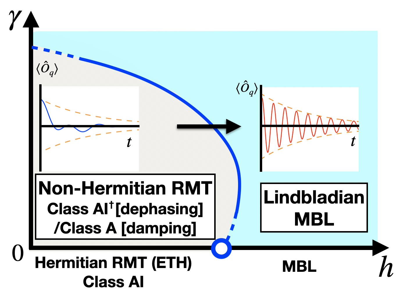
In this work, we show that an unconventional localization occurs for dissipative systems as a spectral transition of the Lindbladian super-operator (rather than the Hamiltonian), which alters the coherent dynamics. In fact, spectral statistics in the middle of the spectrum are characterized by the universality of the non-Hermitian RMT for weak disorder and by the localization of the Lindbladian eigenstates for strong disorder (see Fig. 1). We call the latter unique open dissipative localization as the Lindbladian MBL. Deep in the Lindbladian MBL regime, quantum coherence exhibits a rigid decay whose rate is essentially determined by the decoherence rate for a single-spin system and stabilized at a roughly constant value against the variations of interaction terms and the magnetic field. This rigidity of the decay rate is attributed to localization of off-diagonal degrees of freedom in the Lindbladian eigenstates. The behavior is distinct from interaction-induced many-body decoherence for weak disorder, where eigenmodes with many different frequencies and decay rates govern the dynamics. Using a prototypical Ising model with a dephasing- or damping-type of dissipation, we numerically demonstrate the transition with, e.g., the complex spacing distributions of eigenvalues and the operator-space entanglement entropy (OSEE) of eigenstates.

We consider a one-dimensional Ising model with transverse and longitudinal fields under dissipation. The dynamics is described by the Lindblad equation with $\hbar=1$ Lindblad (1976):

Here, the Hamiltonian is given by $\hat{H}=\sum_{i=1}^{L-1}J\hat{\sigma}_{i}^{z}\hat{\sigma}_{i+1}^{z}+\sum_{i=1}^{L}g\hat{\sigma}_{i}^{x}+\sum_{i=1}^{L}h_{i}\hat{\sigma}_{i}^{z},$ where $h_{i}$ is taken randomly from $[-h,+h]$. Without dissipation, $\hat{H}$ exhibits MBL for sufficiently strong disorder Imbrie (2016a, b). We consider two types of dissipation, namely dephasing $\hat{\Gamma}_{l}=\sqrt{\gamma}\hat{\sigma}^{z}_{l},$ and damping $\hat{\Gamma}_{l}={\sqrt{\frac{\gamma}{2}}}\hat{\sigma}^{-}_{l}$ with $\hat{\sigma}^{-}_{l}=\hat{\sigma}^{x}_{l}-i\hat{\sigma}^{y}_{l}$. Below we mainly consider the case with weak dissipation ($\gamma<g$). The case with large dissipation $(\gamma>g)$ is discussed at the Discussion section.

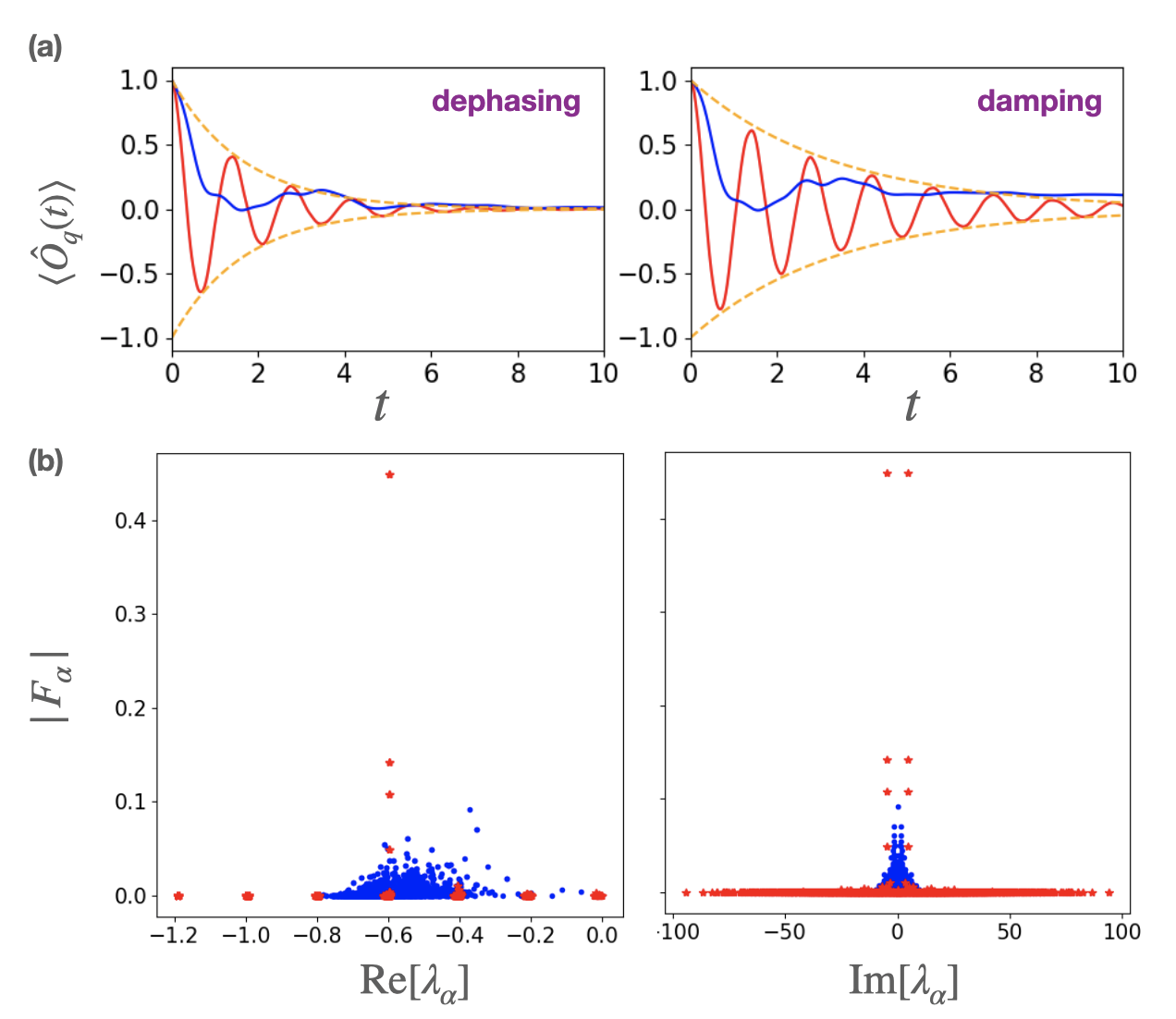
We first discuss the time evolution of coherence measured by $\hat{O}_{q}=\bigotimes_{k=L-q+1}^{L}\hat{\sigma}_{k}^{x}$ starting from an initial state $\hat{\rho}_{q}=\ket{\psi_{q}}\bra{\psi_{q}}$, where $\ket{\psi_{q}}=(\ket{\downarrow}_{1}\cdots\ket{\downarrow}_{L-q})\left(\frac{\ket{\uparrow}_{L-q+1}\cdots\ket{\uparrow}_{L}+\ket{\downarrow}_{L-q+1}\cdots\ket{\downarrow}_{L}}{\sqrt{2}}\right).$ This choice corresponds to measuring the single-spin coherence for $q=1$ and macroscopic coherence of the Greenberger-Horne-Zeilinger state for $q=L$. In Fig. 2(a), we show the time evolution of the quantum expectation value of $\braket{\hat{O}_{q}(t)}$ (not averaged over disorder) for different values of disorder strength. While $\braket{\hat{O}_{q}(t)}$ rapidly relaxes to a stationary value for small $h$, it exhibits a slower oscillatory decay for large $h$. Only for the latter case, the decay rate is almost stabilized at around $2\gamma q~{}(\gamma q)$ for dephasing (damping) pol , which is explained by the decoherence rate for a single-spin system and robust against many-body interactions (see Supplemental Materials Sup ).

To understand the distinction between two regimes, we consider the spectral decomposition of the dynamics Gong and Hamazaki (2022):

where $\hat{R}_{\alpha}$ ($\hat{L}_{\alpha}$) is a right (left) eigenstate of the Lindbladian super-operator $\mathcal{L}$ with an eigenvalue $\lambda_{\alpha}\in\mathbb{C}$ nor . For weak disorder, many eigenstates for different $\lambda_{\alpha}$ contribute to the dynamics, i.e., $|F_{\alpha}|$ in Eq. (2) spreads over many $\alpha$ (see Fig. 2(b)), indicating complicated many-body decoherence characterized by a large number of frequencies and decay rates. On the other hand, for strong disorder, peaks in $|F_{\alpha}|$ appear for several eigenstates in the middle of the spectrum with the other $|F_{\alpha}|$ being vanishingly small. These selected eigenstates lead to an oscillatory decay governed by only a few frequencies and a rigid decay rate despite many-body interactions.

The distinctive behavior of the behavior of $|F_{\alpha}|$ discussed above is attributed to the different regimes characterized by the spectral statistics of the Lindbladian super-operator. For weak disorder, we find that the statistics obey the non-Hermitian RMT. In particular, the trace factors appearing in Eq. (2) in the middle of the spectrum and away from the real axis are described as

and

where $\mathcal{A}_{\hat{O}}$, $\mathcal{B}_{\hat{\rho}}$, and $\mathcal{C}$ are smooth functions of $\lambda_{\alpha}$, and $r_{\alpha}$ and $r^{\prime}_{\alpha}$ are complex random variables normalized as $\mathbb{E}[|r_{\alpha}|]=\mathbb{E}[|r_{\alpha}^{\prime}|]=1$. These forms indicate that every energy eigenstate fluctuates randomly within a sufficiently small two-dimensional eigenvalue window where $\mathcal{A}_{\hat{O}}(\lambda_{\alpha})$, $\mathcal{B}_{\hat{\rho}}(\lambda_{\alpha})$, and $\mathcal{C}(\lambda_{\alpha})$ are almost constant. In this sense, Eqs. (3)-(5) constitute a dissipative generalization of the (off-diagonal) ETH for Hermitian systems, which states that $\braket{E_{a}}{\hat{O}}{E_{b}}$ fluctuates within the small energy windows around $E_{a}$ and $E_{b}$ according to (Hermitian) RMT Khatami et al. (2013) for quantum chaotic systems cla .

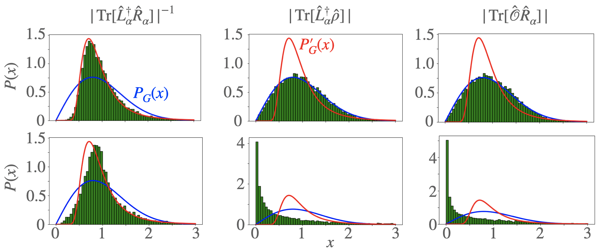
Notably, the distributions of $r_{\alpha}$ and $r^{\prime}_{\alpha}$ obey the non-Hermitian RMT universality Ginibre (1965); Chalker and Mehlig (1998); Mehlig and Chalker (2000). Specifically, the distributions $P(r_{\alpha})$ and $P(r^{\prime}_{\alpha})$ are described by $P_{G}(x):=P(|r_{\alpha}^{G}|=x)=\frac{\pi}{2}xe^{-\frac{\pi}{2}x^{2}},$ which is obtained from the Porter-Thomas distribution, and $P_{G}^{\prime}(x):=P(|r_{\alpha}^{G^{\prime}}|=x)=\frac{32}{\pi^{2}x^{5}}e^{-\frac{4}{\pi x^{2}}},$ which is obtained from the results of a complex Ginibre ensemble Bourgade and Dubach (2019); rea . As shown in Fig. 3, these results are valid for our model with weak disorder, but invalid for strong disorder pea .

As detailed in Supplemental Material Sup , $|\mathrm{Tr}[\hat{O}\hat{R}_{\alpha}]|$ and $|\mathrm{Tr}[\hat{L}_{\alpha}^{\dagger}\hat{\rho}]|$ decrease, and $|\mathrm{Tr}[\hat{L}_{\alpha}^{\dagger}\hat{R}_{\alpha}]|^{-1}$ increases with increasing $L$. Furthermore, $|\mathrm{Tr}[\hat{L}_{\alpha}^{\dagger}\hat{R}_{\alpha}]|^{-1}$ for small $h$ is almost proportional to the dimension $D=2^{L}$ of the Hilbert space. We also find $\mathrm{Tr}[\hat{L}_{\alpha}^{\dagger}\hat{\rho}]\propto D^{-1}$ for small $h$. These scalings agree with the prediction of the non-Hermitian RMT. On the other hand, for strong $h$, the scaling behavior differs from the RMT for both cases. Note that the scaling behavior is not simple for $|\mathrm{Tr}[\hat{O}\hat{R}_{\alpha}]|$ because of the locality of the operator and that of the Lindbladian. In this case, we argue that $|\mathrm{Tr}[\hat{O}\hat{R}_{\alpha}]|\sim e^{-c^{\prime}|\lambda_{\alpha}|}\>(c^{\prime}>0)$ Sup .

The above discussions indicate that, for weak disorder, eigenstates within a small eigenvalue window fluctuate randomly for $|\mathrm{Tr}[\hat{R}_{\alpha}^{\dagger}\hat{L}_{\alpha}]|^{-1},|\mathrm{Tr}[\hat{L}_{\alpha}^{\dagger}\hat{\rho}]|,$ and $|\mathrm{Tr}[\hat{O}\hat{R}_{\alpha}]|$. Consequently, $F_{\alpha}$ also behaves randomly without irregular eigenstates as shown in Fig. 2(b), resulting in many-body decoherence governed by many modes with different frequencies and decay rates. The above discussion establishes the previously unknown connection between dissipative quantum chaos and many-body decoherence in terms of eigenstates with the RMT universality.

We next discuss the strong-disorder case. We start from the phenomenological picture with quasi-local bits Huse et al. (2014) in the MBL phase without dissipation. Then, the Hamiltonian reads

where $\tilde{h}_{l}\simeq h_{l}$, and $J_{lm},J_{lmn},\cdots$ decay exponentially for any far apart two-site indices. The local integral of motion $\hat{\tau}_{l}^{z}$ has a large overlap with $\hat{\sigma}_{l}^{z}$. The Hamiltonian $\hat{H}$ has eigenstates labeled by the eigenvalues $\pm 1$ of $\hat{\tau}_{l}^{z}$, i.e., $\ket{\tau_{1}\cdots\tau_{L}}$. We can express $\hat{\sigma}_{l}$ by $\hat{\tau}_{l}$ as $\hat{\sigma}_{l}^{z}=\sum_{\alpha=x,y,z}Z_{l}^{\alpha}\hat{\tau}_{l}^{\alpha}+\sum_{jk}\sum_{\alpha,\beta=x,y,z}G_{l,jk}^{\alpha\beta}\hat{\tau}_{j}^{\alpha}\hat{\tau}_{k}^{\beta}+\text{(higher order terms)}$, where $Z_{l}^{z}=1-\mathrm{O}((g/h)^{2})$, $Z_{l}^{x,y}=\mathrm{O}(g/h)$, and $G_{l,jk}^{\alpha\beta}$ rapidly decays as a function of $|l-j|$ and $|l-k|$. Also, $G_{l,jk}^{\alpha\beta}=\mathrm{O}((g/h)^{2})$ Imbrie (2016a, b). A similar representation is obtained for $\hat{\sigma}_{l}^{-}$. Then, the Lindbladian reads $\mathcal{L}[\hat{\rho}]=-i[\hat{H},\hat{\rho}]+\mathcal{L}_{Z}+\mathcal{L}_{P}$, where $\mathcal{L}_{Z}=\frac{{Z_{l}^{z}}^{2}}{2}\sum_{l}\left[2\hat{\Gamma}_{l}^{\prime}\hat{\rho}\hat{\Gamma}_{l}^{\prime{\dagger}}-{\left\{\hat{\Gamma}_{l}^{\prime{\dagger}}\hat{\Gamma}_{l}^{\prime},\hat{\rho}\right\}}\right]$ with $\hat{\Gamma}_{l}^{\prime}=\sqrt{\gamma}\hat{\tau}_{l}^{z}$ (dephasing) or $\hat{\Gamma}_{l}^{\prime}=\sqrt{\frac{\gamma}{2}}\hat{\tau}_{-}^{z}$ (damping), and $\mathcal{L}_{P}$ denotes the remaining perturbation.

We briefly discuss the case of dephasing-type dissipation here (see Supplemental Material for details and the case of damping-type dissipation Sup ). The eigenstates of $-i[\hat{H},\hat{\rho}]+\mathcal{L}_{Z}$ can be written as $\hat{R}_{\alpha}=\hat{L}_{\alpha}=\ket{\tau_{1}\cdots\tau_{L}}\bra{\tau_{1}^{\prime}\cdots\tau_{L}^{\prime}}=\hat{\phi}_{1}^{\alpha_{1}}\otimes\hat{\phi}_{2}^{\alpha_{2}}\otimes\cdots\otimes\hat{\phi}_{L}^{\alpha_{L}}$. Here, $\otimes$ represents the tensor product for different localized bits $\hat{\tau}_{i}$, and $\hat{\phi}_{l}^{\alpha_{l}}=\ket{\tau_{l}}\bra{\tau_{l}^{\prime}}$. Specifically, we take $\hat{\phi}^{1}=(\hat{\phi}^{2})^{\dagger}=\ket{+1}\bra{-1}$, $\hat{\phi}^{3}=\ket{+1}\bra{+1}$, and $\hat{\phi}^{4}=\ket{-1}\bra{-1}$, where $\ket{\pm 1}$ is the eigenstate of $\hat{\tau}^{z}$ with an eigenvalue $\pm 1$. The corresponding eigenvalues are $-i\sum_{l}2\tilde{h}_{l}(\delta_{\alpha_{l},1}-\delta_{\alpha_{l},2})-i(\text{small terms including }J_{lm},\cdots)-\sum_{l}2{Z_{l}^{z}}^{2}\gamma(\delta_{\alpha_{l},1}+\delta_{\alpha_{l},2})$.

When we add $\mathcal{L}_{P}$, $\hat{\phi}_{l}^{3}$ and $\hat{\phi}_{l}^{4}$ in different eigenstates are mixed, since the eigenvalue difference is almost zero in this case. In contrast, $\hat{\phi}_{l}^{1}$ and $\hat{\phi}_{l}^{2}$ are typically stable under first-order perturbation, since the transition matrix elements over the eigenvalue difference are $\mathrm{O}(\gamma g/h^{2})\ll 1$ Sup . It follows then that while diagonal degrees of freedom (DDOF) $\hat{\phi}_{l}^{3}$ and $\hat{\phi}_{l}^{4}$ can delocalize, off-diagonal degrees of freedom (ODDOF) $\hat{\phi}_{l}^{1}$ and $\hat{\phi}_{l}^{2}$ can localize. Consequently, eigenstates are not fully mixed, and the RMT prediction breaks down. In the dynamics of coherence considered in Fig. 2 Coh , only the modes with $\alpha_{L-q+1}=\cdots=\alpha_{L}=1$ or 2 contribute to $F_{\alpha}$, and the other modes make negligible contributions to $F_{\alpha}$. The decay rate is then stabilized, and the system evades many-body decoherence. In particular, the decay rate becomes $\sim 2q\gamma(1-\mathrm{O}((g/h)^{2}))$. For the damping case, the decay rate is similarly stabilized at $\sim q\gamma(1-\mathrm{O}((g/h)^{2}))$.

The stabilized dynamics of the coherence (transverse relaxation) is understood from the nontrivial Lindbladian localization of the ODDOF, which cannot be captured by the classical effective rate equation Fischer et al. (2016); Medvedyeva et al. (2016) used for describing the slow longitudinal relaxation in previous studies. Indeed, the DDOF that govern the longitudinal relaxation Fischer et al. (2016); Medvedyeva et al. (2016) are delocalized. A detailed discussion of the difference between longitudinal and transverse relaxation is given in Supplemental Material Sup .

A few remarks are in order here. First, the delocalization/localization of DDOF/ODDOF is reasonable because they undergo zero/strong random fields $\sim 0/\pm 2\tilde{h}_{l}$ in the matrix representation of the Lindbladian Sup . Second, the localization of ODDOF indicates the emergence of a quasi-local weak symmetry Buča and Prosen (2012); Albert and Jiang (2014) $\hat{U}_{w}$ of the Lindbladian, i.e., $\hat{U}_{w}\mathcal{L}[\hat{\rho}]\hat{U}_{w}^{\dagger}=\mathcal{L}[\hat{U}_{w}\hat{\rho}\hat{U}_{w}^{\dagger}]$, which block-diagonalizes the Lindbladian. Third, as for the discussion of the Hermitian MBL, it is not easy to show the existence of localization and the precise transition point when we consider higher-order perturbations and resonant states Šuntajs et al. (2020); Morningstar et al. (2022); Sels (2021). We leave it as a future problem to investigate larger system sizes.

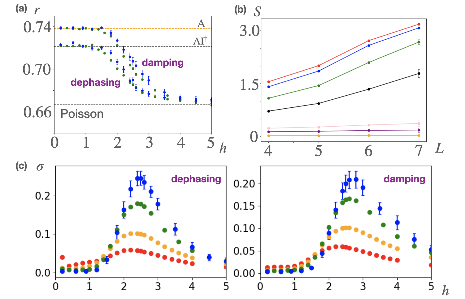
To strengthen evidence for the Lindbladian MBL transition, we calculate the spacing statistics of complex eigenvalues Grobe et al. (1988); Grobe and Haake (1989); Markum et al. (1999); Akemann et al. (2019); Hamazaki et al. (2019, 2020); Jaiswal et al. (2019); Wang et al. (2020); Sá et al. (2020a, b); Tzortzakakis et al. (2020); Huang and Shklovskii (2020); Mudute-Ndumbe and Graefe (2020); Luo et al. (2021); Sá et al. (2021); Rubio-García et al. (2022); Prasad et al. (2022); García-García et al. (2022), particularly the complex spacing ratio $r=\mathbb{E}_{\alpha}\left[\left|\frac{\lambda_{\alpha}-\lambda_{\alpha}^{\mathrm{N}}}{\lambda_{\alpha}-\lambda_{\alpha}^{\mathrm{NN}}}\right|\right]$ Sá et al. (2020a) as a function of $h$ in Fig. 4(a), where $\lambda_{\alpha}^{\mathrm{N}}$ and $\lambda_{\alpha}^{\mathrm{NN}}$ are the nearest and the next-nearest neighbor eigenvalues of $\lambda_{\alpha}$ on the complex plane. For small $h$, $r$ is close to $r_{\mathrm{AI^{\dagger}}}\simeq 0.721$ and $r_{\mathrm{A}}\simeq 0.737$ for dephasing-type and damping-type, respectively. Here, $r_{\mathrm{AI^{\dagger}}}$ and $r_{\mathrm{A}}$ denote the complex spacing ratio for the non-Hermitian random matrices belonging to classes $\mathrm{AI}^{\dagger}$ and $\mathrm{A}$. On the other hand, $r$ decreases with increasing $h$ and eventually approaches the value for the Poisson distribution, $r_{\mathrm{Po}}=2/3$ str . Note that Ref. Yusipov and Ivanchenko (2021) reports a similar eigenvalue transition for different disordered models, but with no mention to eigenstates and the change in the dynamics associated with localization.

We next consider the operator-space entanglement entropy (OSEE) $S_{\alpha}$ Prosen and Pižorn (2007); Pižorn and Prosen (2009) of the (right) eigenstate $\hat{R}_{\alpha}$ for bipartition at the middle of the system $l=\lfloor L/2\rfloor$ OSE . Figure 4(b) shows the system-size dependence of $S_{\alpha}$ averaged over eigenstates in the middle of the spectrum for different disorder strengths. While the OSEE increases with increasing $L$ for small $h$, its shows a much slower increase for large $h$. This is similar to the entanglement transition of the MBL in a closed system.

To find the transition point, we define the variance $\sigma$ of the OSEE with respect to the eigenstates and show its disorder-strength dependence for various $L$ (Fig. 3(c)). The peak develops as we increase the system size, from which the transition point reads as $h_{c}=2.5\pm 0.1\>(2.7\pm 0.1)$ for dephasing (damping). The peak of $\sigma$ at the transition is a dissipative counterpart of the peak of the variance of the entanglement entropy for the isolated MBL Kjäll et al. (2014).

We have discussed the transition for fixed $\gamma$ with $0<\gamma<g$. In contrast, as detailed in Supplemental Material Sup , by changing $\gamma$ (including $\gamma\geq g$), we numerically find that the critical value $h_{c}(\gamma)$ exhibits non-monotonic behavior. Namely, $h_{c}(\gamma)$ first increases and then decreases. This implies that strong dissipation facilitates the Lindbladian MBL. For sufficiently large $\gamma$, we find the breakdown of the non-Hermitian RMT statistics even for small $h$, as shown in Fig. 1. This indicates that a localized regime appears even for the clean system; however, we leave it as a future problem to investigate this possibility for larger system sizes.

In the opposite limit $\gamma\rightarrow 0$, it is nontrivial whether the Lindbladian MBL transition point $h_{c}(\gamma\rightarrow 0)$ coincides with the Hermitian MBL transition point $h_{\mathrm{H},c}$. We conjecture that these two transition points coincide under certain conditions (see Supplemental Material Sup ).

We have demonstrated that localization of Lindbladian eigenstates can occur in the open quantum many-body systems and stabilizes the decay rate of coherence without many-body decoherence despite interactions, if disorder is sufficiently strong. The weakly disordered phase is characterized by the spectral statistics reflecting the universality of non-Hermitian RMT, and the strongly disordered phase is characterized by the Lindbladian MBL.

Our study raises interesting questions. The nature of the transitions between the RMT and the Lindbladian MBL phases using larger system sizes needs to be investigated, which may uncover, e.g., a new type of criticality defined by the spectral statistics of super-operators in dissipative systems. It is also interesting to ask whether the delocalization-localization transitions of the spectrum found in this paper occur for models with different types of Hamiltonians (e.g., particle-number-conserving models) and dissipation (e.g., stochastic hopping Diehl et al. (2008); Yusipov et al. (2017); Vakulchyk et al. (2018); Haga et al. (2021)). Furthermore, it is intriguing to clarify the relation between our phases defined by the middle of the spectrum (relevant for transient-time dynamics) and the other types of MBL phenomenology under dissipation, such as the long-time thermalization Fischer et al. (2016); Levi et al. (2016); Medvedyeva et al. (2016); Lüschen et al. (2017); van Nieuwenburg et al. (2017); Morningstar et al. (2022); Sels (2021) and the non-Hermitian MBL Hamazaki et al. (2019).

References

- Srednicki (1994) M. Srednicki, Phys. Rev. E 50, 888 (1994).
- Deutsch (1991) J. M. Deutsch, Phys. Rev. A 43, 2046 (1991).
- Rigol et al. (2008) M. Rigol, V. Dunjko, and M. Olshanii, Nature 452, 854 (2008).
- Rigol (2009) M. Rigol, Phys. Rev. A 80, 053607 (2009).
- Biroli et al. (2010) G. Biroli, C. Kollath, and A. M. Läuchli, Phys. Rev. Lett. 105, 250401 (2010).
- Genway et al. (2012) S. Genway, A. F. Ho, and D. K. K. Lee, Phys. Rev. A 86, 023609 (2012).
- Khatami et al. (2013) E. Khatami, G. Pupillo, M. Srednicki, and M. Rigol, Phys. Rev. Lett. 111, 050403 (2013).
- Steinigeweg et al. (2013) R. Steinigeweg, J. Herbrych, and P. Prelovšek, Phys. Rev. E 87, 012118 (2013).
- Beugeling et al. (2014) W. Beugeling, R. Moessner, and M. Haque, Phys. Rev. E 89, 042112 (2014).
- Kim et al. (2014) H. Kim, T. N. Ikeda, and D. A. Huse, Phys. Rev. E 90, 052105 (2014).
- Beugeling et al. (2015) W. Beugeling, R. Moessner, and M. Haque, Phys. Rev. E 91, 012144 (2015).
- Luitz and Bar Lev (2016) D. J. Luitz and Y. Bar Lev, Phys. Rev. Lett. 117, 170404 (2016).
- Yoshizawa et al. (2018) T. Yoshizawa, E. Iyoda, and T. Sagawa, Phys. Rev. Lett. 120, 200604 (2018).
- Hamazaki and Ueda (2019) R. Hamazaki and M. Ueda, Phys. Rev. E 99, 042116 (2019).
- Khaymovich et al. (2019) I. M. Khaymovich, M. Haque, and P. A. McClarty, Phys. Rev. Lett. 122, 070601 (2019).
- Jansen et al. (2019) D. Jansen, J. Stolpp, L. Vidmar, and F. Heidrich-Meisner, Phys. Rev. B 99, 155130 (2019).
- Nation and Porras (2019) C. Nation and D. Porras, Phys. Rev. E 99, 052139 (2019).
- Sugimoto et al. (2021a) S. Sugimoto, R. Hamazaki, and M. Ueda, Phys. Rev. Lett. 126, 120602 (2021a).
- Fritzsch and Prosen (2021) F. Fritzsch and T. c. v. Prosen, Phys. Rev. E 103, 062133 (2021).
- Sugimoto et al. (2021b) S. Sugimoto, R. Hamazaki, and M. Ueda, arXiv preprint arXiv:2111.12484 (2021b).
- D’Alessio et al. (2016) L. D’Alessio, Y. Kafri, A. Polkovnikov, and M. Rigol, Advances in Physics 65, 239 (2016).
- Mori et al. (2018) T. Mori, T. N. Ikeda, E. Kaminishi, and M. Ueda, Journal of Physics B: Atomic, Molecular and Optical Physics 51, 112001 (2018).
- Haake (2010) F. Haake, Quantum signatures of chaos, Vol. 54 (Springer Science & Business Media, 2010).
- Basko et al. (2006) D. Basko, I. Aleiner, and B. Altshuler, Annals of physics 321, 1126 (2006).
- Žnidarič et al. (2008) M. Žnidarič, T. Prosen, and P. Prelovšek, Phys. Rev. B 77, 064426 (2008).
- Pal and Huse (2010) A. Pal and D. A. Huse, Phys. Rev. B 82, 174411 (2010).
- Gogolin et al. (2011) C. Gogolin, M. P. Müller, and J. Eisert, Phys. Rev. Lett. 106, 040401 (2011).
- Bardarson et al. (2012) J. H. Bardarson, F. Pollmann, and J. E. Moore, Phys. Rev. Lett. 109, 017202 (2012).
- Iyer et al. (2013) S. Iyer, V. Oganesyan, G. Refael, and D. A. Huse, Phys. Rev. B 87, 134202 (2013).
- Huse et al. (2013) D. A. Huse, R. Nandkishore, V. Oganesyan, A. Pal, and S. L. Sondhi, Phys. Rev. B 88, 014206 (2013).
- Serbyn et al. (2013) M. Serbyn, Z. Papić, and D. A. Abanin, Phys. Rev. Lett. 111, 127201 (2013).
- Huse et al. (2014) D. A. Huse, R. Nandkishore, and V. Oganesyan, Phys. Rev. B 90, 174202 (2014).
- Kjäll et al. (2014) J. A. Kjäll, J. H. Bardarson, and F. Pollmann, Phys. Rev. Lett. 113, 107204 (2014).
- Nandkishore and Huse (2015) R. Nandkishore and D. A. Huse, Annual Review of Condensed Matter Physics 6, 15 (2015).
- Bera et al. (2015) S. Bera, H. Schomerus, F. Heidrich-Meisner, and J. H. Bardarson, Phys. Rev. Lett. 115, 046603 (2015).
- Ponte et al. (2015) P. Ponte, Z. Papić, F. Huveneers, and D. A. Abanin, Phys. Rev. Lett. 114, 140401 (2015).
- Potter et al. (2015) A. C. Potter, R. Vasseur, and S. A. Parameswaran, Phys. Rev. X 5, 031033 (2015).
- Schreiber et al. (2015) M. Schreiber, S. S. Hodgman, P. Bordia, H. P. Lüschen, M. H. Fischer, R. Vosk, E. Altman, U. Schneider, and I. Bloch, Science 349, 842 (2015).
- Luitz et al. (2015) D. J. Luitz, N. Laflorencie, and F. Alet, Physical Review B 91, 081103(R) (2015).
- Vosk et al. (2015) R. Vosk, D. A. Huse, and E. Altman, Phys. Rev. X 5, 031032 (2015).
- Smith et al. (2016) J. Smith, A. Lee, P. Richerme, B. Neyenhuis, P. W. Hess, P. Hauke, M. Heyl, D. A. Huse, and C. Monroe, Nature Physics 12, 907 (2016).
- Choi et al. (2016) J.-y. Choi, S. Hild, J. Zeiher, P. Schauß, A. Rubio-Abadal, T. Yefsah, V. Khemani, D. A. Huse, I. Bloch, and C. Gross, Science 352, 1547 (2016).
- Imbrie (2016a) J. Z. Imbrie, Phys. Rev. Lett. 117, 027201 (2016a).
- Imbrie (2016b) J. Z. Imbrie, Journal of Statistical Physics 163, 998 (2016b).
- Khemani et al. (2017) V. Khemani, S. P. Lim, D. N. Sheng, and D. A. Huse, Phys. Rev. X 7, 021013 (2017).
- Alet and Laflorencie (2018) F. Alet and N. Laflorencie, Comptes Rendus Physique 19, 498 (2018).
- Lukin et al. (2019) A. Lukin, M. Rispoli, R. Schittko, M. E. Tai, A. M. Kaufman, S. Choi, V. Khemani, J. Léonard, and M. Greiner, Science 364, 256 (2019).
- Abanin et al. (2019) D. A. Abanin, E. Altman, I. Bloch, and M. Serbyn, Rev. Mod. Phys. 91, 021001 (2019).
- Syassen et al. (2008) N. Syassen, D. M. Bauer, M. Lettner, T. Volz, D. Dietze, J. J. Garcia-Ripoll, J. I. Cirac, G. Rempe, and S. Dürr, Science 320, 1329 (2008).
- Barreiro et al. (2011) J. T. Barreiro, M. Müller, P. Schindler, D. Nigg, T. Monz, M. Chwalla, M. Hennrich, C. F. Roos, P. Zoller, and R. Blatt, Nature 470, 486 (2011).
- Yan et al. (2013) B. Yan, S. A. Moses, B. Gadway, J. P. Covey, K. R. Hazzard, A. M. Rey, D. S. Jin, and J. Ye, Nature 501, 521 (2013).
- Barontini et al. (2013) G. Barontini, R. Labouvie, F. Stubenrauch, A. Vogler, V. Guarrera, and H. Ott, Phys. Rev. Lett. 110, 035302 (2013).
- Labouvie et al. (2015) R. Labouvie, B. Santra, S. Heun, S. Wimberger, and H. Ott, Phys. Rev. Lett. 115, 050601 (2015).
- Patil et al. (2015) Y. S. Patil, S. Chakram, and M. Vengalattore, Phys. Rev. Lett. 115, 140402 (2015).
- Gao et al. (2015) T. Gao, E. Estrecho, K. Bliokh, T. Liew, M. Fraser, S. Brodbeck, M. Kamp, C. Schneider, S. Höfling, Y. Yamamoto, F. Nori, Y. Kivshar, A. Truscott, R. Dall, and E. Ostrovskaya, Nature 526, 554 (2015).
- Labouvie et al. (2016) R. Labouvie, B. Santra, S. Heun, and H. Ott, Phys. Rev. Lett. 116, 235302 (2016).
- Lüschen et al. (2017) H. P. Lüschen, P. Bordia, S. S. Hodgman, M. Schreiber, S. Sarkar, A. J. Daley, M. H. Fischer, E. Altman, I. Bloch, and U. Schneider, Phys. Rev. X 7, 011034 (2017).
- Raftery et al. (2014) J. Raftery, D. Sadri, S. Schmidt, H. E. Türeci, and A. A. Houck, Phys. Rev. X 4, 031043 (2014).
- Tomita et al. (2017) T. Tomita, S. Nakajima, I. Danshita, Y. Takasu, and Y. Takahashi, Science advances 3, e1701513 (2017).
- Lapp et al. (2019) S. Lapp, J. Ang’ong’a, F. A. An, and B. Gadway, New Journal of Physics 21, 045006 (2019).
- Takasu et al. (2020) Y. Takasu, T. Yagami, Y. Ashida, R. Hamazaki, Y. Kuno, and Y. Takahashi, Progress of Theoretical and Experimental Physics 2020, 12A110 (2020).
- Bouganne et al. (2020) R. Bouganne, M. B. Aguilera, A. Ghermaoui, J. Beugnon, and F. Gerbier, Nature Physics 16, 21 (2020).
- Keßler et al. (2021) H. Keßler, P. Kongkhambut, C. Georges, L. Mathey, J. G. Cosme, and A. Hemmerich, Phys. Rev. Lett. 127, 043602 (2021).
- Noel et al. (2021) C. Noel, P. Niroula, A. Risinger, L. Egan, D. Biswas, M. Cetina, A. V. Gorshkov, M. Gullans, D. A. Huse, and C. Monroe, arXiv preprint arXiv:2106.05881 (2021).
- Nandkishore et al. (2014) R. Nandkishore, S. Gopalakrishnan, and D. A. Huse, Phys. Rev. B 90, 064203 (2014).
- Johri et al. (2014) S. Johri, R. Nandkishore, and R. Bhatt, arXiv preprint arXiv:1405.5515 (2014).
- Fischer et al. (2016) M. H. Fischer, M. Maksymenko, and E. Altman, Phys. Rev. Lett. 116, 160401 (2016).
- Levi et al. (2016) E. Levi, M. Heyl, I. Lesanovsky, and J. P. Garrahan, Phys. Rev. Lett. 116, 237203 (2016).
- Medvedyeva et al. (2016) M. V. Medvedyeva, T. Prosen, and M. Znidaric, Phys. Rev. B 93, 094205 (2016).
- van Nieuwenburg et al. (2017) E. P. van Nieuwenburg, J. Y. Malo, A. J. Daley, and M. H. Fischer, Quantum Science and Technology 3, 01LT02 (2017).
- Morningstar et al. (2022) A. Morningstar, L. Colmenarez, V. Khemani, D. J. Luitz, and D. A. Huse, Phys. Rev. B 105, 174205 (2022).
- Sels (2021) D. Sels, arXiv preprint arXiv:2108.10796 (2021).
- (73) References Morningstar et al. (2022); Sels (2021) analyzed the Liouvillian gap of the Lindbladian super-operator, which is different from the middle of the spectrum of the Lindbladian considered in our work as an analogue with the Hermitian case.
- Hamazaki et al. (2019) R. Hamazaki, K. Kawabata, and M. Ueda, Phys. Rev. Lett. 123, 090603 (2019).
- Lindblad (1976) G. Lindblad, Comm. Math. Phys. 48, 119 (1976).
- (76) In addition to the exponential decay whose rate is proportional to , the coherence may have a polynomial decay factor due to interactions as in Hermitian cases Serbyn and Abanin (2017); Abanin et al. (2019). However, this factor is negligible compared with the exponential decay.
- (77) See Supplemental Material for details of the relaxation dynamics, structures of the overlaps concerning eigenstates, a phenomenology of the Lindbladian MBL phase, and dissipation dependence of the Lindbladian MBL transition point.
- Gong and Hamazaki (2022) Z. Gong and R. Hamazaki, arXiv preprint arXiv:2202.02011 (2022).
- (79) We normalize the eigenstates such that is satisfied except for the stationary states, for which and .
- (80) We note that a similar conjecture is given for classical Markovian systems, as discussed in Supplemental Material Sup .
- Ginibre (1965) J. Ginibre, Journal of Mathematical Physics 6, 440 (1965).
- Chalker and Mehlig (1998) J. T. Chalker and B. Mehlig, Phys. Rev. Lett. 81, 3367 (1998).
- Mehlig and Chalker (2000) B. Mehlig and J. T. Chalker, Journal of Mathematical Physics 41, 3233 (2000).
- Bourgade and Dubach (2019) P. Bourgade and G. Dubach, Probability Theory and Related Fields , 1 (2019).
- (85) While the analytical formula for ensembles different from a complex Ginibre ensemble (e.g., a real Ginibre ensemble and an ensemble with transposition symmetry Hamazaki et al. (2020)) is not known, we have numerically confirmed this distribution. If is real, then and can be taken to be real, and their distributions may be different from the case of complex eigenvalues. We here do not consider real eigenvalues because their fractions vanish in the limit of large system size.
- (86) The peaks at for and with large indicate that the eigenstates of the Lindbladian and those of or can be orthogonal in the operator space for the localized regime.
- (87) Precisely speaking, this result is for the coherence measured by, e.g., or its product for different ’s. While the dynamics of or its product may be slightly different from that for , its difference becomes smaller if is increased. See Supplemental Material Sup for further discussions and additional numerical results.
- Buča and Prosen (2012) B. Buča and T. Prosen, New Journal of Physics 14, 073007 (2012).
- Albert and Jiang (2014) V. V. Albert and L. Jiang, Phys. Rev. A 89, 022118 (2014).
- Šuntajs et al. (2020) J. Šuntajs, J. Bonča, T. Prosen, and L. Vidmar, Physical Review E 102, 062144 (2020).
- (91) Specifically, let us consider the real part and the absolute value of the imaginary part of , and sort each of them independently as and . We use only those modes whose eigenvalues satisfy and .
- Grobe et al. (1988) R. Grobe, F. Haake, and H.-J. Sommers, Phys. Rev. Lett. 61, 1899 (1988).
- Grobe and Haake (1989) R. Grobe and F. Haake, Phys. Rev. Lett. 62, 2893 (1989).
- Markum et al. (1999) H. Markum, R. Pullirsch, and T. Wettig, Phys. Rev. Lett. 83, 484 (1999).
- Akemann et al. (2019) G. Akemann, M. Kieburg, A. Mielke, and T. c. v. Prosen, Phys. Rev. Lett. 123, 254101 (2019).
- Hamazaki et al. (2020) R. Hamazaki, K. Kawabata, N. Kura, and M. Ueda, Phys. Rev. Research 2, 023286 (2020).
- Jaiswal et al. (2019) A. B. Jaiswal, A. Pandey, and R. Prakash, EPL (Europhysics Letters) 127, 30004 (2019).
- Wang et al. (2020) K. Wang, F. Piazza, and D. J. Luitz, Phys. Rev. Lett. 124, 100604 (2020).
- Sá et al. (2020a) L. Sá, P. Ribeiro, and T. c. v. Prosen, Phys. Rev. X 10, 021019 (2020a).
- Sá et al. (2020b) L. Sá, P. Ribeiro, T. Can, and T. c. v. Prosen, Phys. Rev. B 102, 134310 (2020b).
- Tzortzakakis et al. (2020) A. F. Tzortzakakis, K. G. Makris, and E. N. Economou, Phys. Rev. B 101, 014202 (2020).
- Huang and Shklovskii (2020) Y. Huang and B. I. Shklovskii, Phys. Rev. B 101, 014204 (2020).
- Mudute-Ndumbe and Graefe (2020) S. Mudute-Ndumbe and E.-M. Graefe, New Journal of Physics 22, 103011 (2020).
- Luo et al. (2021) X. Luo, T. Ohtsuki, and R. Shindou, Phys. Rev. Lett. 126, 090402 (2021).
- Sá et al. (2021) L. Sá, P. Ribeiro, and T. c. v. Prosen, Phys. Rev. B 103, 115132 (2021).
- Rubio-García et al. (2022) A. Rubio-García, R. Molina, and J. Dukelsky, SciPost Physics Core 5, 026 (2022).
- Prasad et al. (2022) M. Prasad, H. K. Yadalam, C. Aron, and M. Kulkarni, Phys. Rev. A 105, L050201 (2022).
- García-García et al. (2022) A. M. García-García, L. Sá, and J. J. M. Verbaarschot, Phys. Rev. X 12, 021040 (2022).
- (109) For too strong , further decreases and becomes smaller than .
- Yusipov and Ivanchenko (2021) I. Yusipov and M. Ivanchenko, arXiv preprint arXiv:2112.06214 (2021).
- Prosen and Pižorn (2007) T. c. v. Prosen and I. Pižorn, Phys. Rev. A 76, 032316 (2007).
- Pižorn and Prosen (2009) I. Pižorn and T. c. v. Prosen, Phys. Rev. B 79, 184416 (2009).
- (113) To define the OSEE, we consider a vector representation of , i.e., , where because of the normalization condition. The entire system with the enlarged Hilbert space spanned by can be separated into two parts as , where and with being the complement of the region . Using the reduced density matrix , we define the OSEE as .
- Diehl et al. (2008) S. Diehl, A. Micheli, A. Kantian, B. Kraus, H. Büchler, and P. Zoller, Nature Physics 4, 878 (2008).
- Yusipov et al. (2017) I. Yusipov, T. Laptyeva, S. Denisov, and M. Ivanchenko, Phys. Rev. Lett. 118, 070402 (2017).
- Vakulchyk et al. (2018) I. Vakulchyk, I. Yusipov, M. Ivanchenko, S. Flach, and S. Denisov, Phys. Rev. B 98, 020202 (2018).
- Haga et al. (2021) T. Haga, M. Nakagawa, R. Hamazaki, and M. Ueda, Phys. Rev. Lett. 127, 070402 (2021).
- Weinberg and Bukov (2017) P. Weinberg and M. Bukov, SciPost Phys. 2, 003 (2017).
- Weinberg and Bukov (2019) P. Weinberg and M. Bukov, SciPost Phys 7, 97 (2019).
- Serbyn and Abanin (2017) M. Serbyn and D. A. Abanin, Phys. Rev. B 96, 014202 (2017).