Limitation on the Student-$t$ Linear Regression Model

In regression analysis, outliers in a linear regression model can jeopardize the results by the ordinary least squares (OLS) estimator. The Student-$t$ linear regression model, designed as a linear regression model with the error term having t-distribution, is one of the common methods to solve the outlier problem (Lange et al., 1989). While the Student-$t$ linear regression model has been widely adopted, most studies apply it without careful theoretical consideration.

Bayesian robustness modeling using heavy tailed distributions, which include $t$-distribution, provides the theoretical solution for the outlier problem. For a simple Bayesian model, when both the prior distribution and the likelihood of an observation are normal distributions, the posterior distribution is also a normal distribution, and the posterior mean is a weighted average of the mean of prior distribution and the observation. When the prior distribution and the observation are located far from each other and follow a normal distribution, the posterior distribution is far from both pieces of information; this is called $conflict$. For example, when a single observation $x=15$ follows $N(\mu,1)$ and the prior of the location parameter follows $N(0,1)$, then the posterior distribution follows $N(7.5,0.5)$. In this case, the posterior distribution is not suggested by either the prior distribution or the observation.

For this problem, Dawid (1973) formally provides the theoretical resolution of the conflict between the prior distribution and the data, also known as conflict of information. He uses the pure location model in which the scale parameter is given and clarifies how an outlier is automatically ignored in the posterior distribution when the outlier follows a heavy-tailed distribution. This result occurs because we believe the information about the prior distribution more than we believe the observation.

O’Hagan (1990) presents the concept of $credence$, which measures the degree of the tail’s information. As Andrade and O’Hagan (2006) mention, credence represents how much we are prepared to believe in one source of information rather than another in the case of conflict; it is represented by the index of a regularly varying function. Andrade and O’Hagan (2011) show that in a univariate model, many observations that are located close enough create a larger credence, which equals the sum of each credence of the observations. When an outlier is far from the group of non-outliers with the same heavy-tailed distribution, the information of the group of non-outliers creates larger credibility or credence. Thus, the posterior distribution is located closer to the non-outliers, and is robust against the outlier. Andrade and O’Hagan (2011) establish sufficient conditions for robust modeling against a single outlier in $n$ samples for a univariate model using regular variation theory. The sufficient condition requires the minimum number of non-outliers to be robust against an outlier. O’Hagan and Pericchi (2012) review previous studies on the resolution of the conflict.

O’Hagan (1988) applies heavy-tailed modeling to a Student-$t$ linear regression model without an intercept term under the pure location structure and demonstrates its robustness. For the model without the intercept term, the outlier unconditionally conflicts with non-outliers. Therefore, a univariate model can be directly applied. By contrast, as Peña et al. (2009) mention, we need to be careful about the outlier in the $x$-direction for the model with an intercept term. Peña et al. (2009) show when the outliers in the $x$-direction reach infinity, the result of a Student-$t$ linear model does not enable robustness. Peña et al. (2009) examine the phenomenon using Kullback–Leibler divergence, and propose a down-weighting method that assigns a lower weight to outliers. As Andrade and O’Hagan’s (2011) show the heavy-tail modeling using $t$-distribution is a partial robust modeling. Thus the location-scale modeling completely cannot ignore outliers. Gagnon et al. (2020) theoretically develop a robust linear regression model using a super heavy tailed distribution, which is heavier than $t$-distribution and provides a wholly robust modeling. He et al. (2021), Andrade (2022), and Gagnon and Hayashi (2023) provided theoretical consideration for the Student-$t$ linear regression model. Although the Student-$t$ linear regression model provides partial robustness, the model is widely applied. Thus, it is quite important to clarify how the model works as a robust model.

Our study investigates the conditions for the Student-$t$ linear model with an intercept term for an outlier in the $y$-direction by extending Andrade and O’Hagan’s (2011) conditions. For this purpose, first, we investigate the range in which there is a conflict between an outlier and non-outliers, which is the necessary condition to apply heavy-tail modeling. Then, we clarify the condition of the model’s robustness.

Heavy-tail modeling as a resolution of a conflict between an outlier and non-outliers works when the outlier and the mean of the group of non-outliers are located far enough, and the sufficient condition for the number of non-outliers is satisfied. A linear regression model provides the mean of $y$ conditioned on $x$. Thus, the conflict of information in a linear regression model with an intercept term occurs when an outlier is located far from the regression line, and non-outliers lie close to the regression line created from non-outliers.

The left panel in Figure 1 shows the case in which the outlier conflicts with the group of non-outliers. The figure shows that the outlier is located far from the regression line by OLS. In this case, the Student-$t$ linear regression model is robust against the outlier in the $y$-direction. This is because the information of the conditional distribution of the outlier is less credible than that for the grouped non-outlier data, under the assumption of the same degrees of freedom of $t$-distribution for all data, which represent $credence$. Non-outliers in the left panel of Figure 1 are close to each other and create a large credence, while the outlier does not belong to the regression line suggested by the grouped data and creates a small credence. Meanwhile, as shown in the right panel of Figure 1, when the outlier is in the $x$-direction, which is called the leverage point, all data, including the outlier, are sufficiently close to the regression line, and create larger credence than the regression line without the outlier, which is presented by the dotted line in Figure 1. In this case, the straight line in the right panel of Figure 1 has larger credence than the dotted line does.

The rest of the paper is organized as follows. In Section 2, we provide the condition for the existence of conflict between an outlier and non-outliers in the Student-$t$ linear regression model. Section 3 shows the sufficient conditions for the Student-$t$ linear regression model. Section 4 presents simulation results in a simple linear regression model. Section 5 concludes.

To examine the limitation of the robustness for the Student-$t$ linear model with an intercept term, we consider the following linear regression model. The dependent variable $\bf y$ is an $n\times 1$ vector, the independent variable $\bf X$ is an $n\times(k+1)$ full-rank matrix, $\bf\beta$ is a $(k+1)\times 1$ vector, and $\bf u$ is an $n\times 1$ vector assumed to be independent and identically distributed:

$\displaystyle\bf{y=X\beta+u},$

(1)

where

$$\bf X\it=\left[\begin{array}[]{cccc}1&X_{11}&\ldots&X_{k1}\\ \vdots&\vdots&\ddots&\vdots\\ 1&X_{1n}&\ldots&X_{kn}\end{array}\right].\\$$

Consider the residual of the result from OLS for the model in equation (1):

$\displaystyle\bf{y=X\hat{\beta}_{ols}+e},$

(2)

where

$$\bf e^{\prime}\it=\left[\begin{array}[]{c}e^{1}_{/out},\ldots,e^{n-1}_{/out},e_{out}\end{array}\right],\\$$

and subscripts ${/out}$ and ${out}$ show a non-outlier and an outlier, respectively.

According to Cook and Weiberg (1982) and Chatterjee and Hadi (1988), the prediction or hat matrix, $\bf\hat{y}=Hy$, is given by

$\displaystyle\bf H=X(X^{\it{T}}\bf X)^{\rm{-1}}\bf X.$

(3)

Then the residual is defined as

$\displaystyle\bf{e}=(\bf{I}_{\it n}-\bf{H})\bf{y}.$

(4)

The element of the hat matrix for the model with the intercept term, the ($i,j$)-th element of $\bf H$, $h_{ij}$ is described as

$\displaystyle h_{ij}=\frac{1}{n}+\bf(x_{\it{i}}-\bar{x})^{\it{T}}\bf(\tilde{X}^{\it{T}}\tilde{X})^{-1}(x{{}_{\it{j}}}-\bar{x})\quad(\it i,j=\rm 1,2,\ldots,\it n),$

(5)

where

$$\bf\widetilde{X}\it=\left[\begin{array}[]{ccc}X_{11}-\bar{X}_{1}&\ldots&X_{k1}-\bar{X}_{k}\\ \vdots&\ddots&\vdots\\ X_{1n}-\bar{X}_{1}&\ldots&X_{kn}-\bar{X}_{k}\end{array}\right],\\ \bf x_{\it{i}}=\left[\begin{array}[]{c}X_{1i}\\ \vdots\\ X_{ki}\end{array}\right],\\ \bf\bar{x}\it=\left[\begin{array}[]{c}\bar{X}_{1}\\ \vdots\\ \bar{X}_{k}\end{array}\right],\\$$

and $\bar{X}_{l}=\Sigma_{i=1}^{n}X_{li}/n\quad(l=1,\ldots,k)$.

In the model with the intercept term, for the diagonal elements, which are called $leverage$, $1/n$ is the smallest value and 1 is the largest.

$$\frac{1}{n}\leq h_{ii}\leq 1\quad(\it i=\rm 1,2,\ldots,\it n).$$

(6)

Mohammadi (2016) showed the range of the off-diagonal elements with the intercept term as follows:

$$\frac{1}{n}-\frac{1}{2}\leq h_{ij}\leq\frac{1}{2}\quad(\it i\neq j).$$

(7)

Assume that the non-outliers are located close enough to the regression line. If the outlier moves away from the regression line and does so faster than the group of non-outliers does, then the residual $e_{out}$ reaches infinity as the outlier reaches infinity in the $y$-direction. Since non-outliers create combined credence, if one of the non-outliers conflicts with the outlier, then the group of non-outliers conflicts with the outlier. As shown in Figure 1, when an outlier is located close enough to the group of non-outliers in the $x$-direction, they conflict. Therefore, if the partial derivative of $e_{out}$ with respect to $y_{out}$ is larger than the partial derivative of the closest non-outlier’s residual, the outlier conflicts with the group of non-outliers.

We derived the relationship between the Hat matrix and the range of outliers in a linear regression model. Let $n$th the observation be an outlier. Thus, $h^{out}_{nn}$ represents the element of $\bf H$ of an outlier.

$\displaystyle\frac{\partial e_{out}}{\partial y_{out}}>\frac{\partial e^{max}_{/out}}{\partial y_{out}},$

(8)

where subscript ${/out}$ is a non-outlier.

From the definition, the partial derivative of the residual of an outlier, $e_{out}$, and the residual of a non-outlier, $e^{j}_{/out}$, with respect to outlier, $y_{out}$, can be given as

$\displaystyle\frac{\partial e_{out}}{\partial y_{out}}=1-h^{out}_{nn},$

(9)

and

$\displaystyle\frac{\partial e^{j}_{/out}}{\partial y_{out}}=-h_{nj}.$

(10)

To investigate the limitation in which an outlier conflicts with the group of non-outliers, this study examined the location of an outlier as the outlier goes to infinity in the $y$-direction. To examine the condition, we first see if the observation is an outlier in the first stage and then derive the condition if the non-outliers create a group.

The condition that the observation becomes an outlier is expressed as the outlier moves away from the regression line, where the residual $e_{out}$ reaches infinity as the outlier reaches infinity in the $y$-direction.

$\displaystyle\it\frac{\partial e_{out}}{\partial y_{out}}>\frac{\partial e^{j}_{/out}}{\partial y_{out}}\quad\quad$

$\displaystyle\quad\quad(j=1,\ldots,n-1).$

(12)

Substituting equations (9) and (10) into the condition (12), we have

$\displaystyle 1-\it h^{out}_{nn}>-h_{nj}.$

(13)

Using (6), Lemma 1 is obtained.

∎

The outlier moves away from the regression line faster than the group of non-outliers. Therefore, if the partial derivative of $e_{out}$ with respect to $y_{out}$ is larger than the partial derivative of non-outlier residuals, non-outliers create a group against the outlier. To create a group of non-outliers, the following conditions are required:

$\displaystyle\begin{cases}\rm(i)\quad\it\frac{\partial e_{out}}{\partial y_{out}}>\frac{\partial e_{/out}}{\partial y_{out}}\quad\quad&\rm for\quad\it\frac{\partial e_{/out}}{\partial y_{out}}\geq\rm 0,\\ \\ \rm(ii)\quad\it\frac{\partial e_{out}}{\partial y_{out}}>-\frac{\partial e_{/out}}{\partial y_{out}}\quad\quad&\rm for\quad\it\frac{\partial e_{/out}}{\partial y_{out}}<\rm 0.\end{cases}$

(15)

When Lemma 1 holds, condition (i) in (15) holds: To satisfy condition (ii) in (15), we have

$\displaystyle 1-\it h^{out}_{nn}>h_{nj}$

(16)

for $\partial e_{/out}/\partial y_{out}<\rm 0$. By the range of $h_{nj}$, Lemma 2 is obtained.

∎

As Chatterjee and Hadi (1988) denoted, since a Hat matrix is idempotent and symmetric, $h^{out}_{nn}$ can be written as

	$\displaystyle h^{out}_{nn}$	$\displaystyle=$	$\displaystyle(h^{out}_{nn})^{2}+\Sigma_{j=1}^{n-1}(h_{nj})^{2}$		(18)
		$\displaystyle=$	$\displaystyle(h^{out}_{nn})^{2}+(h_{nj})^{2}+\Sigma_{k\neq j}^{n-1}(h_{nk})^{2}$

By arranging (18), we have

$\displaystyle\frac{1}{4}$

$\displaystyle=$

$\displaystyle\left(h^{out}_{nn}-\frac{1}{2}\right)^{2}+(h_{nj})^{2}+\Sigma_{k\neq j}^{n-1}(h_{nk})^{2}.$

(19)

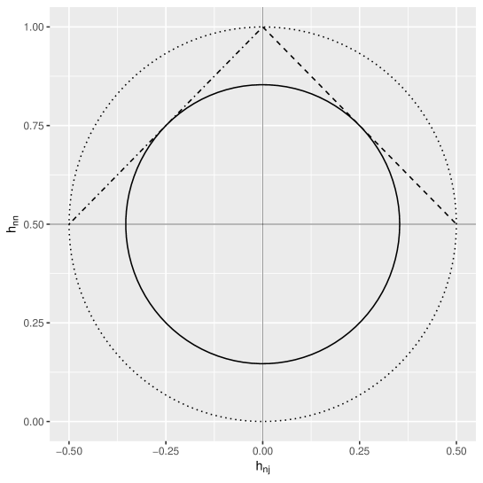
The dashed line and the dot-dashed line in Figure 2 show Lemma 1 and 2 based on the conditions (13) and (16). The dotted circle in Fig 2 shows the case with $\Sigma_{k\neq j}^{n-1}(h_{nk})^{2}=0$, which does not satisfy both Lemma 1 and 2 for $h_{nn}^{out}>0.5$. From the figure, $\Sigma_{k\neq j}^{n-1}(h_{nk})^{2}$ is necessary greater than or equal to $\frac{1}{8}$ to satisfy the conditions of Lemma 1 and 2.

∎

This section investigates the sufficient conditions for a Student-$t$ linear regression model being robust based on Andrade and O’Hagan’s (2011) corollary 4, which shows the conditions for robustness against a single outlier out of $n$ samples in a univariate model. To examine the conditions for the Student-$t$ linear regression model, we adopt the independent Jeffreys priors derived by Fonseca et al. (2008, 2014) under the given degrees of freedom.

As shown in Andrade and O’Hagan (2006), the credence is defined as $c$ for $f(x)\in R_{-c}(c>0)$, where $R_{-c}$ presents that $f(x)$ is regularly varying at $\infty$ with index $c$. For a $t$ distribution, the credence of $t$ distribution with $\gamma$ degrees of freedom is $\gamma+$1 (see Appendix A).

Assume all data, including a single outlier among $n$ observations, are $t$-distributed with degrees of freedom, $\gamma$, $t_{\gamma}(\mu,\sigma)$, which has mean $\mu$ and scale parameter $\sigma$ with $\gamma$ degrees of freedom. As the $t$-distribution is a location-scale family, the likelihood can be denoted as $f(y_{i}|\bf X,\beta,\it\sigma)=\rm 1/\it\sigma\times h[(y_{i}-X^{\prime}_{i}\beta)/\sigma]$. $X^{\prime}_{i}$ is the $i$-th row of $\bf X$.

For simplicity, assume all data have the same likelihood function and the non-outliers are close enough to the conditional mean $X^{\prime}_{i}\beta$. Consider the $n$-th observation is an outlier.

Consider $n$ observations in the present model, and Lemma 1 holds, in which the residual $e_{n}=y_{n}-x^{T}_{n}\beta$ reaches infinity as $y_{n}$ goes to infinity. Then, the following condition holds: $(\gamma+1)<\{n-p\}$.

Then, the posterior distribution partially ignores the outlier:

$$\pi(\beta,\sigma|\mathbf{X},\mathbf{y})\propto\sigma^{\gamma}\pi(\beta,\sigma|\bf{X^{\rm(\it n-\rm 1)}},\mathbf{y}^{\rm(\it n-\rm 1)})\hskip 28.45274pt\textrm{as}\hskip 8.5359pt\it y_{n}\rightarrow\infty,$$

(20)

where the superscript notation ${(n-1)}$ is used to indicate the omission of the $n$-th observation.

When scale parameter $\sigma$ is given, the posterior distribution of $\beta$ in the model is as follows:

	$\displaystyle\pi(\beta|\sigma,\textbf{X}^{(n-1)},\textbf{y}^{(n-1)})$	$\displaystyle\propto$	$\displaystyle\pi(\beta)\cdot\Pi_{i=1}^{n-1}h[(y_{i}-X^{T}_{i}\beta)/\sigma]$
		$\displaystyle\propto$	$\displaystyle\Pi_{i=1}^{n-1}h[(y_{i}-X^{T}_{i}\beta)/\sigma]\in R_{-(n-1)(\gamma+1)}.$

Applying transformation $\tau=\frac{1}{\sigma}\beta$, which is a $p\times$ 1 vector, we obtain

$\displaystyle\pi(\textbf{y}^{(n-1)}|\sigma,\textbf{X}^{(n-1)})$

$\displaystyle=$

$\displaystyle\left(\frac{1}{\sigma}\right)^{n-p-1}\int_{\mathbb{R}^{p}}\Pi_{i=1}^{n-1}h[(y_{i}/\sigma)-X^{T}_{i}\tau]d\tau.$

(22)

When all elements of X are given and bounded, $\int_{\mathbb{R}^{p}}\Pi_{i=1}^{n-1}h[(y_{i}/\sigma)-X^{T}_{i}\tau]d\tau$ in $\sigma$ is $O$(1). Thus, as a function of $\sigma$, it is slowly varying,

$\displaystyle\int_{\mathbb{R}^{p}}\Pi_{i=1}^{n-1}h[(y_{i}/\sigma)-X^{T}_{i}\tau]d\tau\in R_{0}.$

(23)

Thus, the marginal posterior distribution of $\sigma$ given information $\textbf{X}^{(n-1)}$ and $\textbf{y}^{(n-1)}$ becomes

$\displaystyle\pi(\sigma|\textbf{X}^{(n-1)},\textbf{y}^{(n-1)})$

$\displaystyle\propto$

$\displaystyle\pi(\sigma)\cdot\pi(\textbf{y}^{(n-1)}|\sigma,\textbf{X}^{(n-1)})\in R_{-(n-p)}.$

(24)

Again, applying transformation $\tau=\frac{1}{\sigma}\beta$ produces the marginal posterior distribution of $y_{n}$ given information $\textbf{X}^{(n-1)}$ as

	$\displaystyle f(y_{n}|\sigma,\textbf{X}^{(n-1)},\textbf{y}^{(n-1)})\hskip 227.62204pt$		(25)
	$\displaystyle\hskip 71.13188pt=\left(\frac{1}{\sigma}\right)^{n-p}\int_{\mathbb{R}^{p}}h[(y_{n}/\sigma)-X^{T}_{n}\tau]\Pi_{i=1}^{n-1}h[(y_{i}/\sigma)-X^{\prime}_{i}\tau]d\tau.$

When non-outliers are located close enough to the regression line, Andrade and O’Hagan’s (2011) Proposition 1, which gives the convolution of regularly varying densities being distributed as the sum of them, $f*g(x)\sim f(x)+g(x)$, can be applied as $f(y)=h[(y_{n}/\sigma)-X^{T}_{n}\tau]$ and $g(y)=\Pi_{i=1}^{n-1}h[(y_{i}/\sigma)-X^{T}_{i}\tau]$. Since $min((\gamma+1),(n-1)(\gamma+1))=(\gamma+1)$ for $n>2$, when the residual $e_{n}=y_{n}-X^{T}_{n}\beta$ reaches infinity as $y_{n}$ goes to the infinity, we obtain

$\displaystyle\int_{\mathbb{R}^{p}}h[(y_{n}/\sigma)-X^{T}_{n}\tau]\Pi_{i=1}^{n-1}h[(y_{i}/\sigma)-X^{T}_{i}\tau]d\tau\in R_{-(\gamma+1)}.$

(26)

Lemma 1 and 2 show the conditions for the residual $e_{n}=y_{n}-X^{T}_{n}\beta$ reaching infinity as $y_{n}$ goes to infinity. Accordingly, the marginal posterior distribution for $\sigma$ is

$\displaystyle\pi(\sigma|\textbf{y})=\frac{f(y_{n}|\sigma,\textbf{X}^{(n-1)},\textbf{y}^{(n-1)})\pi(\sigma|X^{(n-1)},\textbf{y}^{(n-1)})}{\int_{0}^{\infty}f(y_{n}|\sigma,\textbf{X}^{(n-1)},\textbf{y}^{(n-1)})\pi(\sigma|\textbf{X}^{(n-1)},\textbf{y}^{(n-1)})d\sigma}.$

(27)

Next, consider the case in which $y_{n}$ goes to infinity. As a function of $y_{n}$, the posterior distribution of $f(y_{n}|\sigma,\textbf{X}^{(n-1)},\textbf{y}^{(n-1)})$ takes the form of $\frac{1}{\sigma}g\left(\frac{y_{n}}{\sigma}\right)\in R_{-(\gamma+1)}$. Thus, by the relationship $g\left(\frac{y_{n}}{\sigma}\right)/g\left(y_{n}\right)=\sigma^{(\gamma+1)}$,

$\displaystyle\lim_{y_{n}\rightarrow\infty}\pi(\sigma|\textbf{y})$

$\displaystyle=$

$\displaystyle\frac{\sigma^{\gamma}\pi(\sigma|X^{(n-1)},\textbf{y}^{(n-1)})}{\lim_{y_{n}\rightarrow\infty}\int_{0}^{\infty}\frac{1}{\sigma}g\left(\frac{y_{n}}{\sigma}\right)/g\left(y_{n}\right)\pi(\sigma|\textbf{X}^{(n-1)},\textbf{y}^{(n-1)})d\sigma}.$

(28)

From (24), we obtain

$\displaystyle\pi(\sigma|\textbf{X}^{(n-1)},\textbf{y}^{(n-1)})\propto\sigma^{-(n-p)}l(\sigma).$

(29)

Thus, for the dominator of (28) to exist, $(\gamma+1)<n-p$ must hold. ∎

This study extended Andrade and O’Hagan’s (2011) condition for resolving the outlier problem of the Student-$t$ linear regression model. The model treats outliers as a natural outcome of the data and does not remove them arbitrarily. The condition works when there is conflicting information between outliers and non-outliers. However, in a linear regression model, an outlier does not conflict with non-outliers when the outlier is located far from non-outliers in the $x$-direction. Thus, we first clarified the range of the presence of conflicting information in a linear regression model. Then, we derived the sufficient condition for robustness of the Student-$t$ linear regression model in the above range. Future research should investigate the conditions for many outliers. Furthermore, it would be interesting to extend this study to a model with unknown degrees of freedom for the $t$-distribution.

References

- [1] Andrade, J.A.A. (2022), On the robustness to outliers of the Student-t process, Scandinavian Journal of Statistics.
- [2] Andrade, J.A.A. and O’Hagan, A. (2006), Bayesian robustness modeling using regularly varying distribution. Bayesian Analysis 1, 169–188.
- [3] Andrade, J.A.A. and O’Hagan, A. (2011), Bayesian robustness modelling of location and scale parameters. Scandinavian Journal of Statistics 38(4), 691–711.
- [4] Bingham, N.H., Goldie, C.M., and Teugels, J.L. (1987), Regular Variation. Cambridge University Press, Cambridge.
- [5] Chatterjee, S. and Hadi, A.S. (1988), Sensitivity Analysis in Linear Regression. Wily, New York.
- [6] Cook, R. D. and Weisberg, S. (1982), Residuals and Influence in Regression. New York: Chapman and Hall.
- [7] Dawid, A.P. (1973), Posterior expectations for large observations. Biometrika 60(3), 664–667.
- [8] Fonseca, T.C.O., Ferreira, M.A.R., and Migon, H.S. (2008), Objective Bayesian analysis for the Student- regression model. Biometrika 95(2), 325–333.
- [9] Gagnon, P., Desgagné, A., and Bédard, M. (2020). A New Bayesian Approach to Robustness Against Outliers in Linear Regression. Bayesian Analysis 15, 389–414.
- [10] Gagnon, P. and Hayashi, Y. (2023), Theoretical properties of Bayesian Student-t linear regression. Statistics and Probability Letters 193, 109693.
- [11] He, D., Sun, D., and He, L. (2021), Objective Bayesian analysis for the 21 Student-t linear regression. Bayesian Analysis, 16, 129–145.
- [12] Lange, K.L., Little, R.J.A., and Taylor, J.M.G. (1989), Robust statistical modeling using the t distribution. Journal of the American Statistical Association 84(408), 881–892.
- [13] O’Hagan, (1988), A. Modelling with heavy tails. Bayesian Statistics 3, 345–359.
- [14] O’Hagan, A. (1990), On Outliers and Credence for Location Parameter Inference. Journal of the American Statistical Association , 85, pp.172–176.
- [15] O’Hagan, A. and Pericchi, L. (2012), Bayesian heavy-tailed models and conflict resolution: A review. Brazilian Journal of Probability and Statistics 26(4), 372–401, 2012.
- [16] Peña, D., Zamar, R., and Yan, G. (2009), Bayesian likelihood robustness in linear models. Journal of Statistical Planning Inference 139(7), 2196–2207, 2009.
- [17] Resnick, S.I. (2007), Heavy-tail Phenomena: Probabilistic and Statistical Modeling. Springer, New York.
Appendix A: Regularly varying functions
The tail behavior can be presented by the index of a regularly varying function. The index is defined as follows.
A positive measurable function is regularly varying at with index for an arbitrary positive .