Likelihood Ratio Confidence Sets for
Sequential Decision Making

Nicolas Emmenegger
ETH Zürich
&Mojmír Mutný¹¹footnotemark: 1
ETH Zürich
&Andreas Krause
ETH Zürich Equal contribution.

Abstract

Certifiable, adaptive uncertainty estimates for unknown quantities are an essential ingredient of sequential decision-making algorithms. Standard approaches rely on problem-dependent concentration results and are limited to a specific combination of parameterization, noise family, and estimator. In this paper, we revisit the likelihood-based inference principle and propose to use likelihood ratios to construct any-time valid confidence sequences without requiring specialized treatment in each application scenario. Our method is especially suitable for problems with well-specified likelihoods, and the resulting sets always maintain the prescribed coverage in a model-agnostic manner. The size of the sets depends on a choice of estimator sequence in the likelihood ratio. We discuss how to provably choose the best sequence of estimators and shed light on connections to online convex optimization with algorithms such as Follow-the-Regularized-Leader. To counteract the initially large bias of the estimators, we propose a reweighting scheme that also opens up deployment in non-parametric settings such as RKHS function classes. We provide a non-asymptotic analysis of the likelihood ratio confidence sets size for generalized linear models, using insights from convex duality and online learning. We showcase the practical strength of our method on generalized linear bandit problems, survival analysis, and bandits with various additive noise distributions.

1 Introduction

One of the main issues addressed by machine learning and statistics is the estimation of an unknown model from noisy observations. For example, in supervised learning, this might concern learning the dependence between an input (covariate) $x$ and a random variable (observation) $y$ . In many cases, we are not only interested in an estimate ${\hat{{\theta}}}$ of the true model parameter ${\theta_{\star}}$ , but instead in a set of plausible values that ${\theta_{\star}}$ could take. Such confidence sets are of tremendous importance in sequential decision-making tasks, where uncertainty is used to drive exploration or risk-aversion needs to be implemented, and covariates are iteratively chosen based on previous observations. This setting includes problems such as bandit optimization, reinforcement learning, or active learning. In the former two, the confidence sets are often used to solve the exploration-exploitation dilemma and more generally influence the selection rule (Mukherjee et al.,, 2022), termination rule (Katz-Samuels and Jamieson,, 2020), exploration (Auer,, 2002) and/or risk-aversion (Makarova et al.,, 2021).

Refer to caption — (a) Gaussian $\mathcal{L}$

When we interact with the environment by gathering data sequentially based on previous confidence sets, we introduce correlations between past noisy observations and future covariates. Data collected in this manner is referred to as adaptively gathered (Wasserman et al.,, 2020). Constructing estimators, confidence sets, and hypothesis tests for such non-i.i.d. data comes with added difficulty. Accordingly, and also for its importance in light of the reproducibility crisis (Baker,, 2016), the task has attracted significant attention in the statistics community in recent years (Ramdas et al.,, 2022).

Instead of deriving explicit concentration inequalities around an online estimator, we construct confidence sets implicitly defined by an inclusion criterion that is easy to evaluate in a computationally efficient manner and requires little statistical knowledge to implement. Roughly speaking, given a model $p_{\theta}(y\,|\,x)$ that describes the conditional dependence of the observation $y$ given the covariate $x$ under parameter $\theta$ , we will build sets based on a weighted modification of the sequential likelihood ratio statistic (Robbins et al.,, 1972; Wasserman et al.,, 2020)

R_{t}(\theta):=\frac{\mathcal{L}_{t}(\{{\hat{{\theta}}}_{s}\}_{s=1}^{t})}{\mathcal{L}_{t}(\theta)}:=\frac{\prod_{s=1}^{t}p^{w_{s}}_{{\hat{{\theta}}}_{s}}(y_{s}\,|\,x_{s})}{\prod_{i=1}^{t}p^{w_{s}}_{\theta}(y_{s}\,|\,x_{s})},

(1)

where $\{{\hat{{\theta}}}_{s}\}_{s}$ is a running estimator sequence that we are free to choose, but which may only depend on previously collected data. Parameters $\theta$ for which this statistic is small, i.e., for which $R_{t}(\theta)\leq 1/\alpha$ will be included in the set (and considered plausible). Examples of sets in a parametric and non-parametric setting are shown in Figure 1. The weighting terms $w_{s}\in(0,1]$ are crucial for dealing with inherent irregularities of many conditional observation models but can be flexibly chosen. Classically, these are set to $w_{s}=1$ . The full exposition of our method with choice of estimators and weights is given in Section 2. Apart from being easy to use and implement, our approach also comes with performance guarantees. These sets maintain a provable $1-\alpha$ coverage – a fact we establish using Ville’s inequality for supermartingales (Ville,, 1939), which is known to be essentially tight for martingales (see Howard et al.,, 2018, for a discussion). Therefore, in stark contrast to alternate methods, our confidence sequence is fully data-dependent, making it empirically tighter than competing approaches. Despite the rich history of sequential testing and related confidence sets going back to Wald, (1945) and Robbins et al., (1972), these sets have found little use in the interactive machine learning community, which is a gap we fill in the present paper.

Contributions

In this work, we revisit the idea of using likelihood ratios to generate anytime-valid confidence sets. The main insight is that whenever the likelihood of the noise process is known, the likelihood ratio confidence sets are fully specified. They inherit their geometry from the likelihood function, and their size depends on the quality of our estimator sequence. We critically evaluate the likelihood ratio confidence sets and, in particular, we shed light on the following aspects: Firstly, for generalized linear models, we theoretically analyze the geometry of the LR confidence sets under mild assumptions. We show their geometry is dictated by Bregman divergences of exponential families (Chowdhury et al.,, 2022). Secondly, we show that the size of the confidence set is dictated by an online prediction game. The size of these sets depends on a sequence of estimators $\{{\hat{{\theta}}}_{s}\}_{s=1}^{t}$ that one uses to estimate the unknown parameter ${\theta_{\star}}$ . We discuss how to pick the estimator sequence in order to yield a provably small radius of the sets, by using the Follow-the-Regularized-Leader algorithm, which implements a regularized maximum-likelihood estimator. We prove that the radius of the confidence sets is nearly-worst-case optimal, and accordingly, they yield nearly-worst-case regret bounds when used in generalized linear bandit applications. However, due to their data-dependent nature, they can be much tighter than this theory suggests. Thirdly, we analyze the limitations of classical (unweighted) LR sets when the underlying conditional observation model is not identifiable. In this case, the resulting (inevitable) estimation bias unnecessarily increases the size of the confidence sets. To mitigate this, we propose an adaptive reweighting scheme that decreases the effect of uninformed early bias of the estimator sequence on the size of the sets downstream. The reweighting does not affect the coverage guarantees of our sets and utilizes an elegant connection to (robust) powered likelihoods (Wasserman et al.,, 2020). Finally, thanks to the adaptive reweighting scheme, our sets are very practical as we showcase experimentally. We demonstrate that our method works well with exponential and non-exponential family likelihoods, and in parametric as well as in kernelized settings. We attribute their practical benefits to the fact that they do not depend on (possibly loose) worst-case parameters.

2 The Likelihood Method

The sequential likelihood ratio process (LRP) in (1) is a statistic that compares the likelihood of a given model parameter, with the performance of an adaptively chosen estimator sequence. As noted above, we generalize the traditional definition, which would have $w_{s}\equiv 1$ , and define a corresponding confidence set as

\mathcal{C}_{t}=\left\{\theta\;\middle|\;R_{t}(\theta)\leq 1/\alpha\right\}.

(2)

The rationale is that the better a parameter $\theta$ is at explaining the data $\{(x_{s},y_{s})\}_{s}^{t}$ from the true model ${\theta_{\star}}$ , the smaller this statistic will be, thereby increasing its chances to be included in $\mathcal{C}_{t}$ . When we construct $R_{t}$ , the sequence of $x_{s}$ , $w_{s}$ and ${\hat{{\theta}}}_{s}$ cannot depend on the noisy observation $y_{s}$ . Formally, consider the filtration $(\mathcal{F}_{s})_{s=0}^{\infty}$ with sub- $\sigma$ -algebras $\mathcal{F}_{s}=\sigma(x_{1},\ldots,y_{1},\ldots x_{s},y_{s},x_{s+1})$ . We require that ${\hat{{\theta}}}_{s}$ and $w_{s}$ are $\mathcal{F}_{s-1}$ -measurable. Under these very mild assumptions and with arbitrary weights $w_{s}\in(0,1]$ , we can show coverage, i.e., our (weighted) confidence sets uniformly track the true parameter with probability $1-\alpha$ .

Theorem 1.

The stochastic process $R_{t}({\theta_{\star}})$ in (1) is a non-negative supermartingale with respect to the filtration $(\mathcal{F}_{t})$ and satisfies $R_{0}({\theta_{\star}})\equiv 1$ . In addition, the sequence $\mathcal{C}_{t}$ from (2) satisfies $\mathbb{P}_{\theta_{\star}}\left(\exists t\,:\,{\theta_{\star}}\not\in\mathcal{C}_{t}\right)\leq\alpha.$

The last statement follows by applying Ville’s inequality for super-martingales on $R_{t}({\theta_{\star}})$ . The proof closely follows Wasserman et al., (2020). While coverage is always guaranteed irrespective of the estimator sequence $\{{\hat{{\theta}}}_{s}\}$ , we would like to make the sets as small as possible at fixed coverage, which we do by picking a well-predicting estimator sequence.

2.1 The Estimator Sequence Game

The specification of the LR process (LRP) allows us to choose an arbitrary estimator sequence $\{{\hat{{\theta}}}_{s}\}_{s}$ . To understand the importance of the sequence, let us introduce ${\theta_{\star}}$ to the definition of $R_{t}$ in (1), and divide by $\mathcal{L}_{t}(\{{\hat{{\theta}}}_{s}\}_{s=1}^{t})$ . This gives the equivalent formulation

\mathcal{C}_{t}:=\left\{\theta\leavevmode\nobreak\ \Big{|}\leavevmode\nobreak\ \frac{\mathcal{L}_{t}({\theta_{\star}})}{\mathcal{L}_{t}(\theta)}\leq\frac{1}{\alpha}\frac{\mathcal{L}_{t}({\theta_{\star}})}{\mathcal{L}_{t}(\{{\hat{{\theta}}}_{s}\}_{s=1}^{t})}\leftarrow\text{confidence parameter}\right\}.

We see that the predictor sequence does not influence the geometry of the confidence set, which is fully specified by the likelihood function. We also observe that the ratio on the right-hand side serves as a confidence parameter controlling the size (radius) of the confidence sets measured under the likelihood ratio distance to ${\theta_{\star}}$ . If the confidence parameter goes to zero, only ${\theta_{\star}}$ is in the set. The better the estimator sequence is at predicting the data, the smaller the inclusion threshold, and hence the smaller the sets will ultimately be. Specifically, taking the $\log$ , we would like to minimize

\displaystyle\mathcal{R}_{t}:=\log\frac{\mathcal{L}_{t}({\theta_{\star}})}{\mathcal{L}_{t}(\{{\hat{{\theta}}}_{s}\}_{s=1}^{t})}=\sum_{s=1}^{t}{-\log(p_{{\hat{{\theta}}}_{s}}^{w_{s}}(y_{s}\,|\,x_{s}))}-\sum_{s=1}^{t}{-\log(p_{{\theta_{\star}}}^{w_{s}}(y_{s}\,|\,x_{s}))}.

(3)

The quantity $\mathcal{R}_{t}$ corresponds to a regret in an online prediction game, as will become apparent below.

Online Prediction Game

Online optimization is a mature field in interactive learning (Cesa-Bianchi and Lugosi,, 2006; Orabona,, 2019). The general goal is to minimize a sequence of loss functions as in Eq. (3) and compete against a baseline, which typically is the best-in-hindsight prediction, or – in our case – given by the performance of the fixed parameter ${\theta_{\star}}$ . Specifically, at every timestep $s$ , iteratively, the agent chooses an action ${\hat{{\theta}}}_{s}$ based on $\mathcal{F}_{s-1}$ , and a loss function $f_{s}(\theta)$ is revealed. In most of the online optimization literature, $f_{s}$ can be chosen adversarially. In our prediction game, we know the whole form of loss function $f_{s}(\theta)=-\log(p^{w_{s}}_{\theta}(y_{s}\,|\,x_{s}))$ , as can be seen in (3), and not just $f_{s}({\hat{{\theta}}}_{s})$ . Opposed to traditional assumptions in online prediction, in our case, $f_{s}$ are non-adversarial, but have a stochastic component due to $y_{s}$ . Also, contrary to most instances of online prediction, we do not compare against the best-in-hindsight predictor, but ${\theta_{\star}}$ instead, as this is more meaningful in our setting.

Online Optimization Algorithms

Generally, we seek an algorithm that incurs low regret. Here, we focus on Follow-the-Regularized Leader (FTRL), which corresponds exactly to using regularized maximum likelihood estimation, making it a natural and computationally practical choice. The update rule is defined in Alg. 1 (Line 3). While other algorithms could be considered, FTRL enjoys the optimal regret rate for generalized linear regression as we show later, and is easily implemented. In order to run the algorithm, one requires a sequence of strongly convex regularizers. For now, let us think of it as $\psi_{s}(\theta)=\lambda||\theta||_{2}^{2}$ , which we use in practice. However, one can derive a tighter analysis for a slightly modified, time-dependent regularization strategy for generalized linear models as we show in Sec. 3.3.

2.2 Adaptive Reweighting: Choosing the Right Loss

There is yet more freedom in the construction of the LR, via the selection of the loss function. Not only do we select the predictor sequence, but also the weights of the losses via $w_{t}$ . This idea allows controlling the influence of a particular data point $(x_{t},y_{t})$ on the cumulative loss based on the value of $x_{t}$ . For example, if we know a priori that for a given $x_{t}$ our prediction will be most likely bad, we can opt out of using the pair $(x_{t},y_{t})$ by setting $w_{t}=0$ . Below we will propose a weighting scheme that depends on a notion of bias, which captures how much of the error in predicting $y_{t}$ is due to our uncertainty about ${\hat{{\theta}}}_{t}$ (compared to the uncertainty we still would have knowing ${\theta_{\star}}$ ). Sometimes this bias is referred to as epistemic uncertainty in the literature, while the residual part of the error is referred to as aleatoric. Putting large weight on a data point heavily affected by this bias might unnecessarily increase the regret of our learner (and hence blow up the size of the confidence set). Note that, conveniently, even if we put low weight (zero) on a data point, nothing stops us from using this sample point to improve the estimator sequence in the next prediction round. As we will show below, our reweighting scheme is crucial in defining a practical algorithm for Reproducing Kernel Hilbert Space (RKHS) models and in high signal-to-noise ratio scenarios. Since we do not know ${\theta_{\star}}$ , our strategy is to compute an estimate of the bias of the estimator ${\hat{{\theta}}}_{t}$ and its effect on the value of the likelihood function for a specific $x$ that we played. We use the value of the bias to rescale the loss via $w_{t}$ such that its effect is of the same magnitude as the statistical error (see Algorithm 1; we call this step bias-weighting).

Intuition

To give a bit more intuition, suppose we have a Gaussian likelihood. Then the negative log-likelihood of $(x_{t},y_{t})$ with weighting is proportional to $\frac{w_{t}}{\sigma^{2}}(y_{t}-x_{t}^{\top}{\hat{{\theta}}}_{t})^{2}$ . Now, if $x_{t}$ does not lie in the span of the data points $\{x_{s}\}_{s=1}^{t-1}$ used to compute ${\hat{{\theta}}}_{t}$ , it is in general unavoidable to incur large error, inversely proportional to $\sigma^{2}$ . To see this, let us decompose the projection onto $x_{t}$ as

x_{t}^{\top}({{\hat{{\theta}}}_{t}-{\theta_{\star}}})=\underbrace{x_{t}^{\top}({\hat{{\theta}}}_{t}-\mathbb{E}[{\hat{{\theta}}}_{t}])}_{\text{statistical error}}+\underbrace{x_{t}^{\top}(\mathbb{E}[{\hat{{\theta}}}_{t}]-{\theta_{\star}})}_{\operatorname{bias}_{x_{t}}({\hat{{\theta}}}_{t})},

(4)

where the first term represents the statistical error up to time $t$ , while the second, bias, is deterministic, and independent of the actual realization $y$ , depending only ${\theta_{\star}}$ . Estimators with non-zero bias are biased. Plugging this into the likelihood function, we see that in expectation $\frac{1}{\sigma^{2}}\mathbb{E}[(y_{t}-x_{t}^{\top}{\hat{{\theta}}}_{t})^{2}|\mathcal{F}_{t-1}]\lesssim\frac{1}{\sigma^{2}}{\operatorname{bias}^{2}_{x_{t}}({\hat{{\theta}}}_{t})}+\epsilon^{2}+\frac{C}{t}$ , where $\epsilon^{2}$ is the unavoidable predictive error in expectation (due to a noisy objective) and is a constant independent of $\sigma^{2}$ . $\frac{C}{t}$ is the statistical error, and $C$ is independent of $\sigma^{2}$ . Note that the bias term scales inversely with the variance, and leads to unnecessarily big confidence parameters for small $\sigma^{2}$ .

In fact, the problem is that we use the likelihood to measure the distance between two parameters, but this is only a “good“ distance once the deterministic source of the error (bias) vanishes. For this reason, without weighting, the incurred regret blows up severely in low-noise settings. To counter this, we balance the deterministic estimation bias and noise variance via proper selection of $w_{t}$ . In this case, it turns out that $w_{t}=\frac{\sigma^{2}}{\sigma^{2}+\operatorname{bias}^{2}_{x_{t}}({\hat{{\theta}}}_{t})}$ ensures that the overall the scaling is independent of $\sigma^{2}$ . While the choice of weights $\{w_{s}\}_{s}^{t}$ influences the geometry of the confidence sets, with a good data collection and estimation strategy the bias asymptotically decreases to zero, and hence the weights converge to $1$ .

Bias estimation

In order to generalize this rule beyond Gaussian likelihoods, we need a proper generalization of the bias. Our generalization is motivated by our analysis of generalized linear models, but the method can be applied more broadly. The role of the squared statistical error (variance) is played by the inverse of the smoothness constant of the negative log-likelihood functions $f_{s}$ , denoted by $L$ . This is the usual smoothness, commonly seen in the convex optimization literature. We consider penalized likelihood estimators with strongly convex regularizers (Alg. 1, line 3). For this estimator class, we define the bias via a hypothetical stochastic-error-free estimate ${\hat{{\theta}}}_{t}^{\times}$ , had we access to the expected values of the gradient loss functions (a.k.a. score). We use the first-order optimality conditions and the indicator function of the set $\Theta$ , $i_{\Theta}$ , to define the error-free-estimate ${\hat{{\theta}}}_{t}^{\times}$ , and the bias of the estimator ${\hat{{\theta}}}_{t}$ as

\operatorname{bias}^{2}_{x_{t}}({\hat{{\theta}}}_{t})=(x_{t}^{\top}({\theta_{\star}}-{\hat{{\theta}}}_{t}^{\times}))^{2}\quad\text{with}\quad\mathbb{E}\left[\sum_{s=1}^{t-1}\nabla\log p_{{\hat{{\theta}}}_{t}^{\times}}(y_{s}|x_{s})\right]-\nabla\psi_{t}({\hat{{\theta}}}_{t}^{\times})+i_{\Theta}({\hat{{\theta}}}^{\times}_{t})=0,

(5)

where the expectation denotes a sequence of expectations conditioned on the prior filtration. This notion of bias coincides with the definition of bias in Eq. (4) for the Gaussian likelihood. This quantity cannot be evaluated in general, however, we prove a computable upper bound.

Theorem 2 (Bias estimate).

Let the negative log-likelihood have the form, $-\log p_{\theta}(y_{s}|x_{s})=g(x_{s}^{\top}\theta)$ , where $g:\mathbb{R}\rightarrow\mathbb{R}$ is $\mu$ strongly-convex and let the regularizer be $\psi_{t}(\theta)=\lambda\lvert\lvert\theta\rvert\rvert_{2}^{2}$ making the overall objective strongly convex. Then, defining $\mathbf{{V}}_{t}^{\mu;\lambda}=\sum_{s=1}^{t}\mu x_{s}x_{s}^{\top}+\lambda\mathbf{{I}}$ , we can bound

\operatorname{bias}^{2}_{x}({\hat{{\theta}}}_{t})\leq 2\lambda\lvert\lvert{\theta_{\star}}\rvert\rvert^{2}_{2}x^{\top}(\mathbf{{V}}_{t}^{\mu;\lambda})^{-1}x.

(6)

The proof is deferred to App. A.3, and requires elementary convex analysis.

This leads us to propose the weighting scheme $w_{t}=\frac{1/L}{\operatorname{bias}^{2}_{x_{t}}({\hat{{\theta}}}_{t})+1/L}$ . We justify that this is a sensible choice by analyzing the confidence set on the GLM class in Section 3, which satisfies the smoothness and strong-convexity conditions. We show that this rule properly balances the stochastic and bias components of the error in the regret as in (3). However, this rule is more broadly applicable beyond the canonical representation of GLM or the GLM family altogether.

1:Input: convex set

\Theta\subset\mathbb{R}^{d}

, confidence level

\alpha>0

, likelihood

p_{\theta}(y|x)

, regularizers

\{\psi_{t}\}_{t}

2:for

t\in\mathbb{N}_{0}

{\hat{{\theta}}}_{t}=\arg\min_{\theta\in\Theta}\sum_{s=1}^{t-1}-\log p_{\theta}(y_{s}\,|\,x_{s})+\psi_{t}(\theta)

\triangleright

FTRL

w_{t}=\begin{cases}\frac{1/L}{1/L+\operatorname{bias}^{2}_{x_{t}}({\hat{{\theta}}}_{t})}&\textsc{this work}\\ 1&\textsc{classical}\\ \end{cases}

\triangleright

bias-weighting

\operatorname{bias}_{x_{t}}({\hat{{\theta}}}_{t})

in Eq. (5) or Eq.(6)

\mathcal{C}_{t}=\left\{\theta\in\Theta\;\middle|\;\prod_{s=1}^{t}\frac{p^{w_{s}}_{{\hat{{\theta}}}_{s}}(y_{s}\,|\,x_{s})}{p^{w_{s}}_{\theta}(y_{s}\,|\,x_{s})}\leq\frac{1}{\alpha}\right\}.

\triangleright

Confidence set

6:end for

Algorithm 1 Constructing the LR Confidence Sequence

3 Theory: Linear Models

While the coverage (i.e., “correctness”) of the likelihood ratio confidence sets is always guaranteed, their worst-case size (affecting the “performance”) cannot be easily bounded in general. We analyze the size and the geometry of the LR confidence sequence in the special but versatile case of generalized linear models.

3.1 Generalized Linear Models

We assume knowledge of the conditional probability model $p_{\theta}(y|x)$ , where the covariates $x\in\mathcal{X}\subset\mathbb{R}^{d}$ , and the true underlying model parameter lies in a set $\Theta\subset\mathbb{R}^{d}$ . If $t$ is indexing (discrete) time, then $x_{t}$ is acquired sequentially, and the – subsequently observed – $y_{t}$ is sampled from an exponential family distribution parametrized as

p_{\theta}(y\,|\,x_{t})=h(y)\exp\left(T(y)\cdot x_{t}^{\top}\theta-A(x_{t}^{\top}\theta)\right).

(7)

Here, $A$ is referred to as the log-partition function of the conditional distribution, and $T(y)$ is the sufficient statistic. The function $h$ is the base measure, and has little effect on our further developments, as it cancels out in the LR. Examples of commonly used exponential families (Gaussian, Binomial, Poisson or Weibull) with their link functions can be found in Table 1 in App. A.1.

In order to facilitate theoretical analysis for online algorithms, we make the following assumptions about the covariates $x\in\mathcal{X}$ and the set of plausible parameters $\Theta$ .

Assumption 1.

The covariates are bounded, i.e., $\sup_{x\in\mathcal{X}}\lvert\lvert x\rvert\rvert_{2}\leq 1$ , and the set $\Theta$ is contained in an $\ell_{2}$ -ball of radius $B$ . We will also assume that the log-partition function is strongly convex, that is, that there exists $\mu:=\inf_{z\in[-B,B]}A^{\prime\prime}(z)$ , and that $A$ is L-smooth, i.e. $L:=\sup_{z\in[-B,B]}A^{\prime\prime}(z)$ .

These assumptions are common in other works addressing the confidence sets of GLMs (Filippi et al.,, 2010; Faury et al.,, 2020), who remark that the dependence on $\mu$ is undesirable. However, in contrast to these works, our confidence sets do not use these assumptions in the construction of the sets. We only require these for our theoretical analysis. As these are worst-case parameters, the practical performance can be much better for our sets.

3.2 Geometry and Concentration

Before stating our results, we need to define a distance notion that the convex negative log-likelihoods induce. For a continuously differentiable convex function $f$ , we denote the Bregman divergence as $D_{f}(a,b):=f(a)-f(b)-\nabla f(b)^{\top}(a-b).$ The $\nu$ -regularized sum of log-partition functions is defined as

Z_{t}^{\nu}(\theta):=\sum_{s=1}^{t}w_{s}A(x_{s}^{\top}\theta)+\frac{\nu}{2}\lvert\lvert\theta\rvert\rvert^{2}_{2}.

(8)

This function will capture the geometry of the LR confidence sets. The confidence set size depends mainly on two terms. One refers to a notion of complexity of the space referred to as Bregman information gain: $\Gamma_{t}^{\nu}({\tilde{{\theta}}}_{t})=\log\left(\frac{\int_{\mathbb{R}^{d}}\exp(-\frac{\nu}{2}\lvert\lvert\theta\rvert\rvert^{2}_{2})\mathrm{d}\theta}{\int_{\mathbb{R}^{d}}\exp(-D_{Z_{t}^{\nu}}(\theta,{\tilde{{\theta}}}_{t}))\mathrm{d}\theta}\right)$ , first defined by Chowdhury et al., (2022) as a generalization of the information gain of Srinivas et al., (2009), $\gamma_{t}^{\nu}=\log\left({\det(\sum_{i=1}\frac{\mu}{\nu}x_{i}x_{i}^{\top}+\mathbf{{I}})}\right)$ for Gaussian likelihoods. We will drop the superscript whenever the regularization is clear from context and simply refer to $\gamma_{t}$ . This term appears because one can relate the decay of the likelihood as a function of the Bregman Divergence from ${\theta_{\star}}$ with the performance of a (regularized) maximum likelihood estimator via convex (Fenchel) duality. In particular, if ${\tilde{{\theta}}}_{t}$ is a regularized MLE, $\Gamma_{t}^{\nu}:=\Gamma_{t}^{\nu}({\tilde{{\theta}}}_{t})$ will asymptotically scale as $\mathcal{O}(d\log t)$ (cf. Chowdhury et al.,, 2022, for further discussion). For Gaussian likelihoods and $w_{s}\equiv 1$ , it coincides with the classical information gain independent of ${\tilde{{\theta}}}_{t}$ . The second term that affects the size is the regret $\mathcal{R}_{t}$ of the online prediction game over $t$ rounds we introduced previously in (3). These two parts together yield the following result:

Theorem 3.

Let $\nu>0$ and $\alpha,\delta\in(0,1)$ . For the level $1-\alpha$ confidence set $\mathcal{C}_{t}$ defined in (2) under the GLM in (7), with probability $1-\delta$ , for all $t\geq 1$ , any $\theta\in\mathcal{C}_{t}$ satisfies

\displaystyle D_{Z_{t}^{\nu}}(\theta,{\theta_{\star}})\leq\frac{4L}{\mu}\xi_{t}+2\log\left(\frac{1}{\delta}\right)+2\mathcal{R}_{t},

(9)

where $\xi_{t}=\left(\log\left(\frac{1}{\alpha}\right)+{\nu B^{2}}+\Gamma_{t}^{\nu}\right)$ and $L,\mu$ are defined as above and finally $\mathcal{R}_{t}$ is the regret of the game in Eq. (3).

The set defined via the above divergence does not coincide with the LR confidence set. It is slightly larger due to a term involving $\nu$ (as in Eq. (8)). This is a technical consequence of our proof technique, where the gradient of $Z_{t}^{\nu}$ needs to be invertible, and regularization is added to this end. We note that this $\nu>0$ can be chosen freely. Note that the theorem involves two confidence levels, $\alpha$ and $\delta$ : $\alpha$ is a bound on the Type I error – coverage of the confidence sets – while $\delta$ upper bounds the probability of a large radius – and is therefore related to the power and Type II error of a corresponding hypothesis test. The proof of the theorem is deferred to App. B.2.

To give more intuition on these quantities, let us instantiate them for the Gaussian likelihood case with $w_{s}\equiv 1$ . In this scenario, $Z_{t}^{\nu}(\theta)=\sum_{s=1}^{t}\frac{1}{2\sigma^{2}}\lvert\lvert\theta\rvert\rvert_{x_{s}x_{s}^{\top}}^{2}+\frac{\nu}{2}\lvert\lvert\theta\rvert\rvert_{2}^{2}$ , and the (in this case symmetric) Bregman divergence is equal to $D_{Z_{t}^{\nu}}({\theta_{\star}},\theta)=\frac{1}{2}\lvert\lvert\theta-{\theta_{\star}}\rvert\rvert^{2}_{\mathbf{V}_{t}^{\sigma^{-2};\nu}}$ , where $\mathbf{{V}}_{t}^{\mu;\nu}=\sum_{s=1}^{t}{\mu x_{s}x_{s}^{\top}+\nu\mathbf{I}}$ , which means that our confidence sets are upper bounded by a ball in the same norm as those in the seminal work on linear bandits (Abbasi-Yadkori et al.,, 2011).

3.3 Online Optimization in GLMs: Follow the Regularized Leader

The size of the confidence sets in Theorem 3 depends on the regret of the online prediction game involving the estimator sequence. We now bound this regret when using the Follow-the-Regularized-Leader (FTRL) algorithm in this setting. This high probability bound is novel to the best of our knowledge and may be of independent interest. We state in a weight-agnostic manner first, and then with our particular choice. The latter variant uses a specifically chosen regularizer. In this case, we can track the contribution of each time-step towards the regret separately.

Theorem 4.

Let $\psi_{t}(\theta)=\lambda\lvert\lvert\theta\rvert\rvert_{2}^{2}$ . Assume Assumption 1, and additionally that $A$ is $L$ -smooth everywhere in $\mathbb{R}^{d}$ , and let $w_{t}\in[0,1]$ be arbitrary. Then, with probability $1-\delta$ the regret of FTRL (Alg. 1) satisfies for all $t\geq 1$

\mathcal{R}_{t}\leq\lambda B^{2}+\frac{L}{\mu}(\gamma_{t}^{\lambda}+2\log({1}/{\delta}))+\frac{2L^{2}B^{2}}{\mu}\gamma_{t}^{\lambda}.

(10)

The regret bounds are optimal in the orders of $\gamma_{t}^{\lambda}$ , matching lower bounds of Ouhamma et al., (2021), as for linear models $\gamma_{t}=\mathcal{O}(d\log t)$ . Combining results of Thm. 4 with Thm. 3, we get a confidence parameter that scales with $\mathcal{O}(\sqrt{\gamma_{t}})$ , for confidence sets of the form $||\theta-{\theta_{\star}}||_{\mathbf{{V}}_{t}}$ , which coincides with the best-known confidence sets in this setting in the worst-case (Abbasi-Yadkori et al.,, 2012). The requirement of global $L-$ smoothness can be relaxed to $L-$ smoothness over $\Theta$ . With a more elaborate (but less insightful) analysis, we can show that we achieve a $\tilde{\mathcal{O}}(\gamma_{t})$ bound even in this case. The proofs of these results are deferred to App. C.4, App. C.5 and App. C.6 respectively.

Regret, Weighting and Estimation Bias

Interestingly, the term in Thm. 4 involving the (crude) proxy to the bias – the bound $B$ – is not scaled by the same $L/\mu$ factors as the other terms in the regret bound (10) and in Theorem 3. Namely, the prefactor is $L^{2}/\mu$ instead of $L/\mu$ . This extra dependence manifests itself in the unnecessary penalization through the estimation bias we introduced in Sec. 2.2, particularly in low-noise settings. We addressed this issue by picking the weights $\{w_{t}\}$ . While the above theorem holds for any valid weighting, it does not exhibit the possible improvement from using specific weights.

We argued earlier that the error in prediction should not be measured by the likelihood function if there is deterministic error, since initially, we are fully uncertain about the value of ${\theta_{\star}}^{\top}(\cdot)$ outside the span of previous observations. Of course, if our goal would be to purely pick weights to minimize $\mathcal{R}_{t}$ , then $w_{s}=0$ would lead to zero regret and hence be optimal. However, the likelihood ratio would then be constant, and uninformative. In other words, the associated log-partition Bregman divergence in Theorem 3 would be trivial and not filter out any hypotheses. Clearly, some balance has to be met. With this motivation in mind, we proposed a nonzero weighting that decreases the regret contribution of the bias, namely $w_{t}=\frac{1/L}{1/L+\operatorname{bias}^{2}_{x_{t}}({\hat{{\theta}}}_{t})}$ . The advantage of this choice becomes more apparent when we use the regularizer $\psi_{t}(\theta)=\lambda||\theta||^{2}+A(x_{t}^{\top}\theta)$ to obtain the following result.

Theorem 5.

Let $\psi_{s}(\theta)=\lambda||\theta||^{2}+A(x_{s}^{\top}\theta)$ . Assume Assumption 1, and additionally that $A$ is $L$ -smooth everywhere in $\mathbb{R}^{d}$ , and choose $w_{s}=\frac{1/L}{1/L+\operatorname{bias}_{x_{s}}({\hat{{\theta}}}_{s})^{2}}$ . Additionally, let the sequence of $x_{s}$ be such that, $\sum_{s}(1-w_{s})(f_{s}({\theta_{\star}})-f_{s}(\bar{\theta}_{s+1}))\leq L/\mu\gamma_{t}^{\lambda}$ , where $\bar{\theta}_{s}$ is the FTRL optimizer with the regularizer $\lambda\lvert\lvert\theta\rvert\rvert_{2}^{2}$ from Theorem 4 ¹¹1 Note that $\bar{\theta}_{s+1}$ corresponds to a regularized MLE that did observe the data pair $(x_{s},y_{s})$ .. Then, with probability $1-\delta$ the regret of FTRL (Alg. 1) satisfies for all $t\geq 1$

\mathcal{R}_{t}\leq\lambda B^{2}+\frac{2L}{\mu}\left(\gamma_{t}^{\lambda}+\log\left(\frac{1}{\delta}\right)\right)+\frac{L}{\mu}\sum_{s=1}^{t}\frac{B^{2}}{1/L+\operatorname{bias}^{2}_{x_{s}}({\hat{{\theta}}}_{s})}\Delta\gamma_{s}^{\lambda},

where $\Delta\gamma_{s}^{\lambda}=\gamma_{s+1}^{\lambda}-\gamma_{s}^{\lambda}$ .

One can see that for points where the information gain $\Delta\gamma_{s}$ is large (corresponding to more unexplored regions of the space, where the deterministic source of error is then large), the weighting scheme will make sure that the multiplicative contribution of $B^{2}$ is mitigated, along with having the correct prefactor $L/\mu$ . The reader may wonder how this result is useful when we replace $\operatorname{bias}^{2}_{x_{s}}({\hat{{\theta}}}_{s})$ with the upper bound from Thm. 2. While instructive, our bound still only makes the bias proxy $B^{2}$ appear in front of the information gain $\Delta\gamma_{t}$ , instead of the more desireable bias itself. In the latter case, we could also directly make use of the upper bound and get an explicit result only using an upper bound on the bias. We leave this for future work.

We point out that this choice of $\psi_{s}(\theta)$ in Theorem 5 corresponds to the Vovk-Azoury-Warmuth predictor (Vovk,, 2001; Azoury and Warmuth,, 1999) in the online learning literature. This choice is helpful in order to track the bias contribution more precisely in our proof.

4 Application: Linear and Kernelized Bandits

Our main motivation to construct confidence sets is bandit optimization. A prototypical bandit algorithm – the Upper Confidence Bound (UCB) (Auer,, 2002) – sequentially chooses covariates $x_{s}$ in order to maximize the reward $\sum_{s=1}^{t}r_{\theta_{\star}}(x_{s})$ , where $r_{\theta_{\star}}$ is the unknown pay-off function parametrized by ${\theta_{\star}}$ . UCB chooses the action $x_{s}$ which maximizes the optimistic estimate of the reward in each round, namely

x_{s}=\operatorname*{arg\,max}_{x\in\mathcal{X}}\max_{\theta\in\mathcal{C}_{s-1}}r_{\theta}(x),

(11)

where $\mathcal{C}_{s-1}$ is some confidence set for ${\theta_{\star}}$ , and can be constructed with Algorithm 1 from the first $s-1$ data points. An important special case is when $r_{\theta_{\star}}$ is linear (Abe and Long,, 1999) or modelled by a generalized linear model (Filippi et al.,, 2010). In that case, the inner optimization problem is convex as long as $\mathcal{C}_{s-1}$ is convex. The outer optimization is tractable for finite $\mathcal{X}$ . In the applications we consider, our confidence sets are convex, and we easily solve the UCB oracle using convex optimization toolboxes.

Extension to RKHS

We introduced the framework of LR confidence sets only for finite-dimensional Euclidean spaces. However, it can be easily extended to Reproducing Kernel Hilbert Spaces (RKHS) (Cucker and Smale,, 2002). The definition of the LR process in (1) is still well-posed, but now the sets are subsets of the RKHS, containing functions $f\in\mathcal{H}_{k}$ . An outstanding issue is how to use these sets in downstream applications, and represent them tractably as in Figure 1. Conveniently, even with infinite-dimensional RKHSs, the inner-optimization in (11) admits a Lagrangian formulation, and the generalized representer theorem applies (Schölkopf et al.,, 2001; Mutný and Krause,, 2021). In other words, we can still derive a pointwise upper confidence band as $\operatorname{ucb}(x)=\max_{f\in\mathcal{H}_{k},\lvert\lvert f\rvert\rvert_{k}\leq B,f\in C_{s}}\braket{f,k(x,\cdot)}$ in terms of $\{x_{j}\}_{j=1}^{s}\cup\{x\}$ , leading to a $s+1$ -dimensional, tractable optimization problem.

We also point out that the weighting is even more paramount in the RKHS setting, as the bias never vanishes for many infinite dimensional Hilbert spaces (Mutný and Krause,, 2022). For this purpose, our weighting is of paramount practical importance, as we can see in Figure 2a), where the gray arrow represents the significant improvement from reweighting.

4.1 Instantiation of the Theory for Linear Bandits

Before going to the experiments, we instantiate our theoretical results from Sec. 3 to the important and well-studied special case of linear payoffs. In that case, $r_{\theta}(x)=\langle x,\,\theta\rangle$ and the agent observes $y_{s}=\langle x_{s},\,{\theta_{\star}}\rangle+\eta_{s}$ upon playing action $x_{s}$ , where $\eta_{s}\sim\mathcal{N}(0,\sigma^{2})$ . We are interested in minimizing the so-called cumulative pseudo-regret, namely, $\mathfrak{R}_{t}=\sum_{s=1}^{t}[\langle{x_{\star}},\,{\theta_{\star}}\rangle-\langle x_{s},\,{\theta_{\star}}\rangle]$ , where $x_{\star}$ refers to the optimal action. Using the set from (2) along with Theorem 3 and the FTRL result of Theorem 4 we can get a regret bound for the choice $w_{s}\equiv 1$ .

Theorem 6.

Let $w_{s}\equiv 1$ . For any $\lambda\geq\frac{1}{\sigma^{2}}$ , with probability at least $1-3\delta$ , for all $t\in\mathbb{N}$ we have

\mathfrak{R}_{t}\leq 6\sqrt{t\gamma_{t}^{\lambda}}\left(\sigma\sqrt{\log(1/\delta)+\gamma_{t}^{\lambda}}+\sigma\lambda^{1/2}B+B\sqrt{\gamma_{t}^{\lambda}}\right).

Our results are optimal in both $d$ and $t$ up to constant and logarithmic factors. The proof is deferred to App. D, but is an instantiation of the aforementioned theorems, along with a standard analysis. There, we also compare to the seminal result of Abbasi-Yadkori et al., (2011), which does not suffer from the dependence on $B\sqrt{\gamma_{t}}$ . We attribute this to the incurred bias in the absence of the reweighting scheme.

For the weighted likelihood ratio, we can obtain a result similar to the above, but multiplied by an upper bound on $\sup_{s\geq 1}w_{s}^{-1}$ . This is undesirable, as our experiments will show that the reweighting scheme vastly improves performance. While this could be somewhat mitigated by using the Theorem 5 instead of Theorem 4 to bound the FTRL regret, a better result should be achievable using our weighting scheme that improves upon Theorem 6 and possibly even matches Abbasi-Yadkori et al., (2011) exactly in the worst-case. We leave this for future work.

4.2 Experimental Evaluation

In this subsection, we demonstrate that the practical applicability goes well beyond the Gaussian theoretical result from the previous subsection. In the examples below, we always use the UCB algorithm but employ different confidence sets. In particular, we compare our LR confidence sets for different likelihood families with alternatives from the literature, notably classical sub-family confidence sets (Abbasi-Yadkori et al.,, 2011; Mutný and Krause,, 2021), and the robust confidence set of Neiswanger and Ramdas, (2021). In practice, however, the radius of these confidence sets is often tuned heuristically. We include such sets as a baseline without provable coverage as well. The main take-home message from the experiments is that among all the estimators and confidence sets that enjoy provable coverage, our confidence sets perform the best, on par with successful heuristics. For all our numerical experiments in Figure 2, the true payoff function is assumed to be an infinite dimensional RKHS element. For further details and experiments, please refer to App. E.

Additive Noise Models

Suppose that $r_{\theta_{\star}}$ is linear and we observe $y_{s}=x_{s}^{\top}{\theta_{\star}}+\eta_{s}$ , where $\eta_{s}$ is additive noise, and ${\theta_{\star}}$ is an element of a Hilbert space. We consider classical Gaussian noise as well as Laplace noise in Fig. 2[a), b)]. Notice that in both cases our confidence sets yield lower regret than any other provably valid method. In both cases they are performing as good as heuristic confidence sets with confidence parameter $\beta_{t}\equiv 2\log(1/\delta)$ . The sub-Gaussian confidence sets of Abbasi-Yadkori et al., (2011) (AY 2011) are invalid for the Laplace distribution as it is not sub-Gaussian but only sub-Exponential. For this reason, we compare also with sub-exponential confidence sets derived similarly to those of (Faury et al.,, 2020). The confidence sets of (Neiswanger and Ramdas,, 2021) (NR 2021) perform similarly on Gaussian likelihood, but are only applicable to this setting, as their generalization to other likelihood families involves intractable posterior inference. We note also the difference between the unweighted LR and the weighted one. The examples in Fig. 2 use the true payoff functions $r(x)=-(1.4-3x)\sin(18x)$ , which we model as an element of a RKHS with squared exponential kernel lengthscale $\gamma=6\times 10^{-2}$ on $[0,1.2]$ , which is the baseline function no. 4 in the global optimization benchmark database infinity77 (Gavana,, 2021). Additional experiments can be found in App. E.

Poisson Bandits

A prominent example of generalized linear bandits (GLB) are Poisson bandits, where the linear payoff is scaled by an exponential function. We instantiate our results on a common benchmark problem, and report the results in Fig. 2d). We improve the regret of UCB for GLBs compared to two alternative confidence sets: one that uses a Laplace approximation with a heuristic confidence parameter, and one inspired by considerations in Mutný and Krause, (2021) (MK 2021), also with a heuristic confidence parameter. Note that we cannot compare directly to their provable results in their original form as they do not state them in the canonical form of the exponential family.

Survival Analysis

Survival analysis is a branch of statistics with a rich history that models the lifespan of a service or product (Breslow,, 1975; Cox,, 1997; Kleinbaum and Klein,, 2010). The classical approach postulates a well-informed likelihood model. Here, we use a specific hazard model, where the survival time $T$ is distributed with a Weibull distribution, parametrized by $\lambda$ and $p$ . The rate $\lambda_{\theta}(x)=\exp(x^{\top}\theta)$ differs for each configuration $x$ , and $p$ – which defines the shape of the survival distribution – is fixed and known. We assume that the unknown part is due to the parameter $\theta$ which is the quantity we build a confidence set around to use within the UCB Algorithm. In particular, the probability density of the Weibull distribution is $P(T=t|x)=\lambda_{\theta}(x)pt^{p-1}\exp(-t^{p}\lambda_{\theta}(x))$ . In fact, with $p=2$ , the confidence sets are convex and the UCB rule can be implemented efficiently.

Interestingly, this model admits an alternate linear regression formulation. Namely upon using the transformation $Y=\log T$ , the transformed variables $Y|x$ follow a Gumbel-type distribution, with the following likelihood that can be obtained by the change of variables $P(Y=y|x)=\lambda_{\theta}(x)p\exp(y)^{p}\exp(-\exp(y)^{p}\lambda_{\theta}(x))$ . The expectation over $Y$ allows us to express it as a linear regression problem since $\mathop{{}\mathbb{E}}[Y|x]=-(\theta^{\top}x+\gamma)/p$ , where $\gamma$ is the Euler-Mascheroni constant. More importantly, $Y|x$ is sub-exponential. Hence, this allows us to use confidence sets for sub-exponential variables constructed with the pseudo-maximization technique inspired by Faury et al., (2020). More details on how these sets are derived can be found in App. E. However, these approaches necessarily employ crude worst-case bounds and as can be seen in Figure 2c) the use of our LR-based confidence sequences substantially reduces the regret of the bandit learner.

5 Related Work and Conclusion

Related Work

The adaptive confidence sequences stem from the seminal work of Robbins et al., (1972), who note that these sets have $\alpha$ -bounded Type I error. The likelihood ratio framework has been recently popularized by Wasserman et al., (2020) for likelihood families without known test statistics under the name universal inference. This approach, although long established, is surprisingly uncommon in sequential decision-making tasks like bandits. This might be due to the absence of an analysis deriving the size of the confidence sets (Mutný and Krause,, 2021), a necessary ingredient to obtain regret bounds. We address this gap for generalized linear models. Another reason might be that practitioners might be interested in non-parametric sub-families – a scenario our method does not cover. That being said, many fields such as survival analysis (Cox,, 1997) do have well-informed likelihoods. However, most importantly, if used naively, this method tends to fail when one departs from assumptions that our probabilistic model is identifiable (i.e., $p_{\theta}(\cdot\,|\,x)=p_{{\tilde{{\theta}}}}(\cdot\,|\,x)$ even if $\theta\not={\tilde{{\theta}}}$ ). We mitigate this problem by introducing the scaling parameters $w_{t}$ in Eq. (1) to deal with it.

Prevalent constructions of anytime-valid confidence intervals rely on carefully derived concentration results and for a specific estimator such as the least-squares estimator and noise sub-families such as sub-Gaussian, sub-Bernoulli and sub-Poisson Abbasi-Yadkori et al., (2011); Faury et al., (2020); Mutný and Krause, (2021). Their constructions involve bounding the suprema of collections of self-normalized stochastic processes (Faury et al.,, 2020; Mutný and Krause,, 2021; Chowdhury et al.,, 2022). To facilitate closed-form expressions, worst-case parameters are introduced that prohibitively affect the size of the sets – making them much larger than they need to be.

Chowdhury et al., (2022) use the exact form of the likelihood to build confidence sets for parameters of exponential families. However, their approach is restricted to exponential family distributions. They use self-normalization and mixing techniques to explicitly determine the size of the confidence set and do not use an online learning subroutine as we do here. Neiswanger and Ramdas, (2021) use likelihood ratios for bandit optimization with possibly misspecified Gaussian processes but is not tractable beyond Gaussian likelihoods. The relation between online convex optimization and confidence sets has been noted in so-called online-to-confidence conversions (Abbasi-Yadkori et al.,, 2012; Jun et al.,, 2017; Zhao et al.,, 2022), where the existence of a low-regret learner implies a small confidence set. However, these sets still use potentially loose regret bounds to define confidence sets. Our definition is implicit. We do not necessarily need a regret bound to run our method, as the radius will depend on the actual, instance-dependent performance of the learner.

Conclusion

In this work, we generalized and analyzed sequential likelihood ratio confidence sets for adaptive inference. We showed that with well-specified likelihoods, this procedure gives small, any-time valid confidence sets with model-agnostic and precise coverage. For generalized linear models, we quantitatively analyzed their size and shape. We invite practitioners to explore and use this very versatile and practical methodology for sequential decision-making tasks.

Acknowledgments and Disclosure of Funding

We thank Wouter Koolen and Aaditya Ramdas for helpful discussions as well as for organizing the SAVI workshop where these discussions took place. NE acknowledges support from the Swiss Study Foundation and the Zeno Karl Schindler Foundation. MM has received funding from the Swiss National Science Foundation through NFP75. This publication was created as part of NCCR Catalysis (grant number 180544), a National Centre of Competence in Research funded by the Swiss National Science Foundation.

References

Abbasi-Yadkori et al., (2011) Abbasi-Yadkori, Y., Pál, D., and Szepesvari, C. (2011). Improved algorithms for linear stochastic bandits. In Advances in Neural Information Processing Systems, pages 2312–2320.
Abbasi-Yadkori et al., (2012) Abbasi-Yadkori, Y., Pal, D., and Szepesvari, C. (2012). Online-to-confidence-set conversions and application to sparse stochastic bandits. In Lawrence, N. D. and Girolami, M., editors, Proceedings of the Fifteenth International Conference on Artificial Intelligence and Statistics, volume 22 of Proceedings of Machine Learning Research, pages 1–9, La Palma, Canary Islands. PMLR.
Abe and Long, (1999) Abe, N. and Long, P. M. (1999). Associative reinforcement learning using linear probabilistic concepts. In ICML, pages 3–11. Citeseer.
Auer, (2002) Auer, P. (2002). Using confidence bounds for exploitation-exploration trade-offs. Journal of Machine Learning Research, 3(Nov):397–422.
Azoury and Warmuth, (1999) Azoury, K. S. and Warmuth, M. K. (1999). Relative loss bounds for on-line density estimation with the exponential family of distributions. Machine Learning, 43:211–246.
Baker, (2016) Baker, M. (2016). 1,500 scientists lift the lid on reproducibility. Nature, 533:452–454.
Breslow, (1975) Breslow, N. E. (1975). Analysis of survival data under the proportional hazards model. International Statistical Review / Revue Internationale de Statistique.
Carpentier et al., (2020) Carpentier, A., Vernade, C., and Abbasi-Yadkori, Y. (2020). The elliptical potential lemma revisited. ArXiv, abs/2010.10182.
Cesa-Bianchi and Lugosi, (2006) Cesa-Bianchi, N. and Lugosi, G. (2006). Prediction, Learning, and Games. Cambridge University Press, New York, NY, USA.
Chowdhury et al., (2022) Chowdhury, S. R., Saux, P., Maillard, O.-A., and Gopalan, A. (2022). Bregman deviations of generic exponential families. arXiv preprint arXiv:2201.07306.
Cox, (1997) Cox, D. R. (1997). Some remarks on the analysis of survival data. In Proceedings of the First Seattle Symposium in Biostatistics, pages 1–9. Springer.
Cucker and Smale, (2002) Cucker, F. and Smale, S. (2002). On the mathematical foundations of learning. Bulletin of the American mathematical society, 39(1):1–49.
Faury et al., (2020) Faury, L., Abeille, M., Calauzènes, C., and Fercoq, O. (2020). Improved optimistic algorithms for logistic bandits. In ICML2020: Proceedings of the 37th International Conference on International Conference on Machine Learning.
Filippi et al., (2010) Filippi, S., Cappe, O., Garivier, A., and Szepesvári, C. (2010). Parametric bandits: The generalized linear case. In Advances in neural information processing systems, pages 586–594.
Gavana, (2021) Gavana, A. (2021). infinity global optimization benchmarks and ampgo. http://infinity77.net/global_optimization/index.html#.
Hazan, (2016) Hazan, E. (2016). Introduction to online convex optimization. Found. Trends Optim., 2:157–325.
Hazan et al., (2006) Hazan, E., Agarwal, A., and Kale, S. (2006). Logarithmic regret algorithms for online convex optimization. Machine Learning, 69:169–192.
Howard et al., (2018) Howard, S. R., Ramdas, A., McAuliffe, J., and Sekhon, J. (2018). Time-uniform chernoff bounds via nonnegative supermartingales. Probability Surveys, 17:257–317.
Jun et al., (2017) Jun, K.-S., Bhargava, A., Nowak, R., and Willett, R. (2017). Scalable generalized linear bandits: Online computation and hashing. Advances in Neural Information Processing Systems, 30.
Katz-Samuels and Jamieson, (2020) Katz-Samuels, J. and Jamieson, K. (2020). The true sample complexity of identifying good arms. In Chiappa, S. and Calandra, R., editors, Proceedings of the Twenty Third International Conference on Artificial Intelligence and Statistics, volume 108 of Proceedings of Machine Learning Research, pages 1781–1791. PMLR.
Kleinbaum and Klein, (2010) Kleinbaum, D. G. and Klein, M. (2010). Survival analysis, volume 3. Springer.
Lattimore and Szepesvári, (2020) Lattimore, T. and Szepesvári, C. (2020). Bandit Algorithms. Cambridge University Press.
Makarova et al., (2021) Makarova, A., Usmanova, I., Bogunovic, I., and Krause, A. (2021). Risk-averse heteroscedastic bayesian optimization. In Proc. Neural Information Processing Systems (NeurIPS).
McCullagh, (2018) McCullagh, P. (2018). Generalized linear models. Chapman and Hall.
Mukherjee et al., (2022) Mukherjee, S., Tripathy, A. S., and Nowak, R. (2022). Chernoff sampling for active testing and extension to active regression. In International Conference on Artificial Intelligence and Statistics, pages 7384–7432. PMLR.
Mutný and Krause, (2021) Mutný, M. and Krause, A. (2021). No-regret algorithms for capturing events in poisson point processes. In Meila, M. and Zhang, T., editors, Proceedings of the 38th International Conference on Machine Learning, volume 139 of Proceedings of Machine Learning Research, pages 7894–7904. PMLR.
Mutný and Krause, (2022) Mutný, M. and Krause, A. (2022). Experimental design of linear functionals in reproducing kernel hilbert spaces. In Proc. Neural Information Processing Systems (NeurIPS).
Neiswanger and Ramdas, (2021) Neiswanger, W. and Ramdas, A. (2021). Uncertainty quantification using martingales for misspecified gaussian processes. In Feldman, V., Ligett, K., and Sabato, S., editors, Proceedings of the 32nd International Conference on Algorithmic Learning Theory, volume 132 of Proceedings of Machine Learning Research, pages 963–982. PMLR.
Orabona, (2019) Orabona, F. (2019). A modern introduction to online learning.
Ouhamma et al., (2021) Ouhamma, R., Maillard, O.-A., and Perchet, V. (2021). Stochastic online linear regression: the forward algorithm to replace ridge. In Neural Information Processing Systems.
Ramdas et al., (2022) Ramdas, A., Grünwald, P., Vovk, V., and Shafer, G. (2022). Game-theoretic statistics and safe anytime-valid inference.
Robbins et al., (1972) Robbins, H., Siegmund, D., et al. (1972). A class of stopping rules for testing parametric hypotheses. In Proceedings of the Sixth Berkeley Symposium on Mathematical Statistics and Probability, Volume 4: Biology and Health. The Regents of the University of California.
Schölkopf et al., (2001) Schölkopf, B., Herbrich, R., and Smola, A. (2001). A generalized representer theorem. In Computational learning theory, pages 416–426. Springer.
Srinivas et al., (2009) Srinivas, N., Krause, A., Kakade, S. M., and Seeger, M. W. (2009). Gaussian process optimization in the bandit setting: No regret and experimental design. In International Conference on Machine Learning.
Ville, (1939) Ville, J.-L. (1939). Étude critique de la notion de collectif.
Vovk, (2001) Vovk, V. (2001). Competitive on-line statistics. International Statistical Review, 69.
Wainwright, (2019) Wainwright, M. J. (2019). High-dimensional statistics: A non-asymptotic viewpoint. Cambridge university press.
Wald, (1945) Wald, A. (1945). Sequential tests of statistical hypotheses. Annals of Mathematical Statistics, 16:256–298.
Wasserman et al., (2020) Wasserman, L. A., Ramdas, A., and Balakrishnan, S. (2020). Universal inference. Proceedings of the National Academy of Sciences, 117:16880 – 16890.
Zhao et al., (2022) Zhao, H., Zhou, D., He, J., and Gu, Q. (2022). Bandit learning with general function classes: Heteroscedastic noise and variance-dependent regret bounds. ArXiv, abs/2202.13603.

Appendix A Proofs of Theorem 1 and 2

A.1 GLM Families

Table 1: Examples of exponential family distributions.

Name	$A(z)$	$A^{\prime}(z)$	$T(y)$	$\mu$	$L$
Gaussian	$z^{2}/(2\sigma^{2})$	$z/\sigma^{2}$	$y/\sigma$	$1/\sigma^{2}$	$1/\sigma^{2}$
Poisson	$\exp(z)$	$\exp(z)$	$y$	$\exp(-B)$	$\exp(B)$
Binomial	$\log(1+\exp(z))$	$\frac{1}{1+\exp(-z)}$	$y$	$\mathcal{O}(\exp(-B))$	$1/4$
Weibull	$k\log(z)-\log k$	$k/z$	$y^{k}$	$1/B^{2}$	$\infty$

A.2 Proof of Theorem 1 (Coverage)

Proof.

Starting with $\mathbb{E}\left[R_{t}({\theta_{\star}})\;\middle|\;\mathcal{F}_{t-1}\right]$

		$\displaystyle=$	$\displaystyle\mathbb{E}\left[R_{t-1}({\theta_{\star}})\frac{p^{w_{t}}_{{\hat{{\theta}}}_{t}}(y_{t}\,\|\,x_{t})}{p^{w_{t}}_{{\theta_{\star}}}(y_{t}\,\|\,x_{t})}\;\middle\|\;\mathcal{F}_{t-1}\right]$
		$\displaystyle=$	$\displaystyle R_{t-1}({\theta_{\star}})\int\frac{p^{w_{t}}_{{\hat{{\theta}}}_{t}}(y\,\|\,x_{t})}{p^{w_{t}}_{{\theta_{\star}}}(y\,\|\,x_{t})}p_{{\theta_{\star}}}(y\,\|\,x_{t})\mathrm{d}y$
		$\displaystyle=$	$\displaystyle R_{t-1}({\theta_{\star}})e^{((w_{t}-1)D^{r}_{w_{t}}(p_{{\theta_{\star}}}(x_{t}),p_{{\hat{{\theta}}}_{t}}(x_{t}))}\leq R_{t-1}({\theta_{\star}}).$

The second equality is due to the fact that $R_{t-1}({\theta_{\star}})$ only depends on $x_{1},y_{1}$ through $x_{t-1},y_{t-1}$ . Since ${\hat{{\theta}}}_{t}$ is $\mathcal{F}_{t-1}$ measurable by assumption, $p_{{\hat{{\theta}}}_{t}}$ is a density, and if $w_{t}<1$ , the integral is equal to an exponential of the Rényi-divergence $D^{r}_{w_{t}}(\cdot,\cdot)$ . The negativity of the exponent follows from $w_{t}<1$ and the non-negativity of the divergence. Note that in the "degenerate" case of $w_{t}=1$ , we can easily see that the integral is over a density (cancellation), and hence also bounded by $1$ . The last part of the statement follows easily by using Ville’s inequality for supermartingales. ∎

All the elements of the above proof appear in Wasserman et al., (2020) albeit separately, and not with time-varying powered robust likelihoods.

A.3 Proof of Theorem 2 (Bias)

We will need a gradient characterization of strong-convexity, which we prove in the following lemma.

Lemma 1 (Convexity: Gradient).

Defining

F_{t}(\theta)=-\sum_{s=1}^{t}\mathop{{}\mathbb{E}}_{{\theta_{\star}}}[\nabla\log_{\theta}p(y_{s}\,|\,x_{s})\,|\,\mathcal{F}_{s-1}],

under the assumption $p_{\theta}(y_{s}|x_{s})=-g(x_{s}^{\top}\theta)$ and $g$ is $\mu$ -strongly convex, we have for any $\theta\in\Theta$ :

(F_{t}(\theta)-F_{t}({\theta_{\star}}))^{\top}(\theta-{\theta_{\star}})\geq\lvert\lvert\theta-{\theta_{\star}}\rvert\rvert_{\mathbf{{V}}_{t}^{\mu;0}}^{2}.

Proof.

We assume that $g$ is $\mu$ -strongly convex. Therefore, for any $s\leq t$ , we get the two inequalities

	$\displaystyle g(x_{s}^{\top}\theta)-g(x_{s}^{\top}{\theta_{\star}})$	$\displaystyle\geq g^{\prime}(x_{s}^{\top}{\theta_{\star}})(x_{s}^{\top}\theta-x_{s}^{\top}{\theta_{\star}})+\frac{\mu}{2}\lvert\lvert x_{s}^{\top}{\theta_{\star}}-x_{s}^{\top}\theta\rvert\rvert_{2}^{2}$
	$\displaystyle g(x_{s}^{\top}{\theta_{\star}})-g(x_{s}^{\top}\theta)$	$\displaystyle\geq g^{\prime}(x_{s}^{\top}\theta)(x_{s}^{\top}{\theta_{\star}}-x_{s}^{\top}\theta)+\frac{\mu}{2}\lvert\lvert x_{s}^{\top}{\theta_{\star}}-x_{s}^{\top}\theta\rvert\rvert_{2}^{2}.$

Adding these two together, we obtain

0\geq(g^{\prime}(x_{s}^{\top}{\theta_{\star}})-g^{\prime}(x_{s}^{\top}\theta))(x_{s}^{\top}(\theta-{\theta_{\star}}))+\mu\lvert\lvert\theta-{\theta_{\star}}\rvert\rvert_{x_{s}x_{s}^{\top}}^{2}.

Observing that $-\nabla_{\theta}p_{\theta}(y_{s}\,|\,x_{s})=-g^{\prime}(x_{s}^{\top}\theta)x_{s}$ , we can equivalently write

0\geq(\nabla\log p_{\theta}(y_{s}\,|\,x_{s})-\nabla\log p_{{\theta_{\star}}}(y_{s}\,|\,x_{s}))^{\top}(\theta-{\theta_{\star}}))+\mu\lvert\lvert\theta-{\theta_{\star}}\rvert\rvert_{x_{s}x_{s}^{\top}}^{2}.

This holds for any realization of $y_{s}$ , and hence taking expectations yields

\left(\mathop{{}\mathbb{E}}[\nabla\log p_{{\theta_{\star}}}(y_{s}\,|\,x_{s})\,|\,\mathcal{F}_{s-1}]-\mathop{{}\mathbb{E}}[\nabla\log p_{\theta}(y_{s}\,|\,x_{s})\,|\,\mathcal{F}_{s-1}]\right)^{\top}(\theta-{\theta_{\star}})\geq\mu\lvert\lvert\theta-{\theta_{\star}}\rvert\rvert_{x_{s}x_{s}^{\top}}^{2}.

Summing up over $s\leq t$ and using the definition of $F_{t}$ we get

(F_{t}(\theta)-F_{t}({\theta_{\star}}))^{\top}(\theta-{\theta_{\star}})\geq\lvert\lvert\theta-{\theta_{\star}}\rvert\rvert_{\mathbf{{V}}_{t}^{\mu};0}^{2}.

∎

Notice that the estimator in Alg. 1 has to fulfil the KKT conditions. We will denote the condition for belonging to the set as $h(\theta)\leq B^{2}$ , where $h$ is a squared and twice-differentiable norm (there are many choices beyond $||\cdot||_{2}^{2}$ ). The KKT conditions are

	$\displaystyle\sum_{s=1}^{t}-\nabla_{\theta}\log p_{\theta}(y_{s}\|x_{s})+\nabla\psi_{t}(\theta)+l\nabla h(\theta)=0$		(12)
	$\displaystyle l(h(\theta)-B^{2})=0$
	$\displaystyle l\geq 0,$

where the second and third conditions represent a complementary slackness requirement. Notice that the system of these equations has a unique solution due to the strong-convexity of the objective, and has to attain a unique minimum on a compact convex subset of $\mathbb{R}^{d}$ . Adding the same quantity on both sides of (12) yields

		$\displaystyle\sum_{s=1}^{t}-\mathbb{E}_{\theta_{\star}}[\nabla_{\theta}\log p_{\theta}(y_{s}\|x_{s})\|\mathcal{F}_{s-1}]+\nabla\psi_{t}(\theta)+l\nabla h(\theta)$
	$\displaystyle=\quad$	$\displaystyle\underbrace{\sum_{s=1}^{t}[\nabla_{\theta}\log p_{\theta}(y_{s}\|x_{s})-\mathbb{E}_{\theta_{\star}}[\nabla_{\theta}\log p_{\theta}(y_{s}\|x_{s})\|\mathcal{F}_{s-1}]]}_{:=E_{t}}.$		(13)

This line motivates the definition of the error-free estimator in $\theta^{\times}_{t}$ (6), where $E_{t}$ is set to zero. We will also make use of a fundamental property of the score (gradient of log-likelihood), namely

\mathbb{E}_{y_{t}\sim p_{\theta_{\star}}(\cdot\,|\,x)}[\nabla\log p_{\theta_{\star}}(y_{t}|x_{t})|\mathcal{F}_{t-1}]=0.

(14)

A classical textbook reference for this is e.g. McCullagh, (2018) but any other classical statistics textbook should contain it. Using these observations, we can already prove Theorem 2.

Proof of Theorem 2.

Using the optimality conditions of $\theta_{t}^{\times}$ , $h(\theta)=||\theta||^{2}_{2}$ and $\psi_{t}(\theta)=\lvert\lvert\theta\rvert\rvert_{2}^{2}$ , we obtain the following statements:

		$\displaystyle\sum_{s=1}^{t}-\mathbb{E}_{\theta_{\star}}[\nabla\log p_{\theta^{\times}_{t}}(y_{s}\|x_{s})\|\mathcal{F}_{s-1}]+\lambda\theta^{\times}_{t}+2l\theta^{\times}_{t}=0$
	$\displaystyle\implies$	$\displaystyle\sum_{s=1}^{t}-\mathbb{E}_{\theta_{\star}}[\nabla\log p_{\theta^{\times}_{t}}(y_{s}\|x_{s})\|\mathcal{F}_{s-1}]+\mathbb{E}_{\theta_{\star}}[\nabla\log p_{{\theta_{\star}}}(y_{s}\|x_{s})\|\mathcal{F}_{s-1}]+{\lambda}\theta^{\times}_{t}+2l\theta^{\times}_{t}=0,$

where in the last line we used the property (14). Now, notice that since we know ${\theta_{\star}}$ is generating the data, the best possible explanation without enforcing the constraint and the regularization would be to set $\theta^{\times}_{t}={\theta_{\star}}$ as the cross-entropy is minimized at this point, and the above is just the optimality condition for optimizing the cross-entropy between these two distribution. Of course, this is only in the absence of regularization or constraints i.e. ${\lambda}=0$ . Now, with the regularization constraint, as the true ${\theta_{\star}}$ lies inside the constraint $h(\theta)\leq B^{2}$ , and both the regularization and constraints induce star-shaped sets, their effect is to make $\theta^{\times}_{t}$ smaller in norm than $\theta^{*}$ . This holds generally for any $h$ which is a norm. As a consequence of this consideration, $||\theta^{\times}_{t}||_{2}<B$ , and then the complementary slackness dictates that $l=0$ .

We can therefore proceed with this simplification. Let us use the shorthand $F_{t}(\theta)=\sum_{s=1}^{t}-\mathbb{E}_{\theta_{\star}}[\nabla\log p_{\theta}(y_{s}|x_{s})|\mathcal{F}_{s-1}]$ and compute

	$\displaystyle F_{t}(\theta_{t}^{\times})-F({\theta_{\star}})+\lambda(\theta^{\times}_{t}-{\theta_{\star}})$	$\displaystyle=-\lambda{\theta_{\star}}$
$\displaystyle\implies$	$\displaystyle(\theta_{t}^{\times}-{\theta_{\star}})^{\top}(F_{t}(\theta_{t}^{\times})-F({\theta_{\star}})+\lambda(\theta^{\times}_{t}-{\theta_{\star}}))$	$\displaystyle=-\lambda(\theta^{\times}_{t}-{\theta_{\star}})^{\top}{\theta_{\star}}$
$\displaystyle\stackrel{{\scriptstyle\text{Lemma}\leavevmode\nobreak\ \ref{lemma:convexity-gradient}}}{{\implies}}$	$\displaystyle\lvert\lvert\theta^{\times}_{t}-{\theta_{\star}}\rvert\rvert^{2}_{\mathbf{{V}}_{t}^{\mu,\lambda}}$	$\displaystyle\leq-\lambda(\theta_{t}^{\times}-{\theta_{\star}})^{\top}{\theta_{\star}}.$	(15)

It suffices to apply the Cauchy-Schwarz Inequality and invoke (15):

$\displaystyle\operatorname{bias}_{x_{s}}({\hat{{\theta}}}_{s})^{2}$	$\displaystyle=$	$\displaystyle(x_{s}^{\top}({\hat{{\theta}}}_{t}^{\times}-{\theta_{\star}}))^{2}$
	$\displaystyle\leq$	$\displaystyle\|\|x_{s}\|\|_{(\mathbf{{V}}^{\mu,\lambda}_{t})^{-1}}^{2}\lvert\lvert\theta^{\times}_{t}-{\theta_{\star}}\rvert\rvert^{2}_{\mathbf{{V}}_{t}^{\mu,\lambda}}$
	$\displaystyle\leq$	$\displaystyle\lambda\|\|x_{s}\|\|_{(\mathbf{{V}}^{\mu,\lambda}_{t})^{-1}}^{2}\lambda(\theta_{t}^{\times}-{\theta_{\star}})^{\top}(-{\theta_{\star}})$
	$\displaystyle\leq$	$\displaystyle\lambda\|\|x_{s}\|\|_{(\mathbf{{V}}^{\mu,\lambda}_{t})^{-1}}^{2}\|\|(\theta_{t}^{\times}-{\theta_{\star}})\|\|_{2}\|\|{\theta_{\star}}\|\|_{2}$
	$\displaystyle\leq$	$\displaystyle 2\lambda\|\|x_{s}\|\|_{(\mathbf{{V}}^{\mu,\lambda}_{t})^{-1}}^{2}\|\|{\theta_{\star}}\|\|_{2}^{2},$

where in the last inequality we used $\lvert\lvert\theta^{\times}_{t}\rvert\rvert_{2}\leq\lvert\lvert{\theta_{\star}}\rvert\rvert_{2}$ , due to the regularizer, as explained above. ∎

GLM models

Let us define the processes

S_{t}=\sum_{s=1}^{t}x_{s}T(y_{s})\quad\text{and}\quad W_{t}=\sum_{s=1}^{t}x_{s}A^{\prime}(x_{s}^{\top}{\theta_{\star}}).

In this scenario, an equivalent of (A.3) then involves the gradient of the regularized (unweighted) log-partition function ${Z_{t}^{\lambda}}$ we defined in (8) and is equal to

\sum_{s=1}^{t}A^{\prime}(x_{s}^{\top}\theta)x_{s}+\nabla\psi_{t}(\theta)+l\nabla h(\theta)=\tilde{E}_{t},

(16)

where $\tilde{E}_{t}=S_{t}$ for ${\hat{{\theta}}}_{t}$ and $\tilde{E}_{t}=W_{t}$ for $\theta_{t}^{\times}$ .

Appendix B Proof of Theorem 3 (Bregman Ball Confidence Set)

Proof sketch

We give a quick sketch of the proof. To bound the size of the sets, we will draw inspiration from the i.i.d. parameter estimation analysis of Wasserman et al., (2020) and separate out the likelihood ratio in a part that relates the true parameter with the estimator sequence (i.e. regret), and a part that is independent of the estimator and characterized by a supremum of a stochastic process. We want to show that any point which is far away from the true parameter will eventually not be included in the confidence set anymore. Defining $\mathcal{L}^{(t)}(\{{\hat{{\theta}}}_{s}\}_{s=1}^{t})$ as $\prod_{i=1}^{t}p_{{\hat{{\theta}}}_{i}}^{w_{i}}(y_{i}\,|\,x_{i})$ , we wish to show that for any $\theta$ far from ${\theta_{\star}}$ , we have

\log\frac{1}{R_{t}(\theta)}=\log\frac{\mathcal{L}^{(t)}(\theta)}{\mathcal{L}^{(t)}({\theta_{\star}})}+\log\frac{\mathcal{L}^{(t)}({\theta_{\star}})}{\mathcal{L}^{(t)}(\{{\hat{{\theta}}}_{s}\}_{s=1}^{t})}\leq\log(\alpha),

which is equivalent to saying that $\theta\not\in\mathcal{C}_{t}$ . The second term corresponds to our notion of regret exactly ( $\mathcal{R}_{t}$ , as discussed above). The first term is what we will focus on. We will bound the supremum of $\log\frac{\mathcal{L}^{(t)}(\theta)}{\mathcal{L}^{(t)}({\theta_{\star}})}$ for all $\theta$ sufficiently far away from ${\theta_{\star}}$ . "Far away" will be measured in the Bregman divergence outlined above. Note that this quantity can be expected to be negative, in general, (especially for "implausible" parameters), since with enough data, ${\theta_{\star}}$ should appear much more likely. Writing this ratio out, we will observe that it is equal to

-D_{Z^{0}_{t}}(\theta,{\theta_{\star}})+\underbrace{\langle\theta-{\theta_{\star}},\,{\sum_{s=1}^{t}w_{s}x_{s}({T(y_{s})-\mathop{{}\mathbb{E}}_{{\theta_{\star}}}[T(y_{s})]})}\rangle}_{\approx\tilde{S}_{t}}.

At this point, it will be sufficient to bound the cross term (second term) over the whole of $\Theta$ . We view this supremum as part of the Legendre Fenchel transform of the function $\mathcal{B}_{t}(\lambda)=D_{Z^{\nu}_{t}}({\theta_{\star}}+\lambda,{\theta_{\star}})$ :

\displaystyle\sup_{\lambda\in\mathbb{R}^{d}}\left(\lambda^{\top}\tilde{S_{t}}-\mathcal{B}_{t}(\lambda)\right){=}\left(\mathcal{B}_{t}\right)^{\star}(\tilde{S_{t}})

and harness duality properties of the Bregman divergence, along with known concentration arguments (Chowdhury et al.,, 2022, Theorem A.1).

B.1 Technical Lemmas

We need to introduce the concept of Legendre functions:

Definition 1.

Let $f:\mathbb{R}^{d}\rightarrow\mathbb{R}$ be a convex function and $C=\mathrm{int}(\mathrm{dom}(f))$ . Then, a function is called Legendre if it satisfies

1.

$C$ is non-empty.
2.

$f$ is differentiable and strictly convex on $C$ .
3.

$\lim_{n\rightarrow\infty}\lvert\lvert\nabla f(x_{n})\rvert\rvert=\infty$ for any sequence $(x_{n})_{n}$ with $x_{n}\in C$ for all $n$ and $\lim_{n\rightarrow\infty}x_{n}=x$ for some $x\in\partial C$ .

This means that the gradient has to blow up near the edge of the domain. Note as well that the boundary condition is vacuous if there is no boundary. Legendre functions have some nice properties, most importantly regarding the bijectivity of their gradients (see e.g. Lattimore and Szepesvári, (2020)):

Lemma 2.

For a Legendre function $f:\mathbb{R}^{d}\rightarrow\mathbb{R}$

1.

$\nabla f$ is a bijection between $\mathrm{int}(\mathrm{dom}(f))$ and $\mathrm{int}(\mathrm{dom}(f^{*}))$ with the inverse $(\nabla f)^{-1}=\nabla f^{*}$ .
2.

$D_{f}(x,y)=D_{f^{*}}(\nabla f(y),\nabla f(x))$ for all $x,y\in\mathrm{int}(\mathrm{dom}(f))$ .
3.

The Fenchel conjugate $f^{*}$ is also Legendre.

With this, we can prove a slightly extended result, that appears as Lemma 2.1. in Chowdhury et al., (2022).

Lemma 3.

For a Legendre function $f$ we have the identity

D_{f}(x,y)=(D_{f,x})^{*}(\nabla f(y)-\nabla f(x))

where we define $D_{f,x}(\lambda)=D_{f}(x+\lambda,x)$ .

Notational Shorthands

Remember the model (7), with log-partition function $A$ . We define $A_{s}(\theta)=w_{s}A(x_{s}^{\top}\theta)$ and $T_{s}(y):=w_{s}x_{s}T(y)$ to denote the log-partition function and the response function of the same exponential family distribution, but parametrized by $\theta$ instead of $x_{s}^{\top}\theta$ . That this is a valid parametrization can easily be seen from the likelihood definition. Indeed, denote by $p^{EF}_{\beta}$ the exponential family reward distribution with parameter $\beta$ . Then our model (7) can be seen to satisfy

p_{\theta}(y\,|\,x_{s})=p_{x_{s}^{\top}\theta}(y)=h(y)\exp(T(y)x_{s}^{\top}\theta-A(x_{s}^{\top}\theta))=h(y)\exp(T_{s}(y)^{\top}\theta-A_{s}(\theta)).

Exponentiating the likelihood with a weighting $w_{s}$ gives rise to another exponential family distribution. We can see that

p_{\theta}^{w_{s}}(y\,|\,x_{s})={h}^{w_{s}}(y)\exp(w_{s}T(y)x_{s}^{\top}\theta-w_{s}A(x_{s}^{\top}\theta))={h}^{w_{s}}(y)\exp(T_{s}(y)^{\top}\theta-A_{s}(\theta)).

Note that this does not necessarily integrate to one, but it is easy to see that there is a normalization function $\tilde{h}$ that makes it integrate to one. Therefore, the following is a valid parametrization of an exponential family distribution:

\tilde{h}(y)\exp(T_{s}(y)^{\top}\theta-A_{s}(\theta)).

Additionally, let $A_{0}(\theta)=\frac{\nu}{2}\lvert\lvert\theta\rvert\rvert_{2}^{2}$ be defined on $\mathbb{R}^{d}$ (i.e. a Legendre Function). We will also define the estimator

{\tilde{{\theta}}}_{t}=\left(\nabla Z^{\nu}_{t}\right)^{-1}\left(\sum_{s=1}^{t}T_{s}(y_{s})\right).

This is a well-defined quantity because the gradient will be invertible, by Lemma 2 above.

Conveniently, Chowdhury et al., (2022) prove the following Theorem 7 using an elegant application of the method of mixtures.

Proposition 1 (Theorem 7 in Chowdhury et al., (2022)).

With probability $1-\delta$ , for all $t\in\mathbb{N}$

D_{Z^{\nu}_{t}}({\theta_{\star}},{\tilde{{\theta}}}_{t})\leq\log(1/\delta)+A_{0}({\theta_{\star}})+\Gamma_{t}^{\nu},

where

\Gamma_{t}^{\nu}=\log\left(\frac{\int_{\mathbb{R}^{d}}\exp(-\frac{1}{2}\lvert\lvert\theta\rvert\rvert^{2}_{2})\mathrm{d}\theta}{\int_{\mathbb{R}^{d}}\exp(-D_{Z^{\nu}_{t}}(\theta,{\tilde{{\theta}}}_{t}))\mathrm{d}\theta}\right).

Lastly, we will need the (one-argument) function

\mathcal{B}_{t}(\lambda)=D_{Z_{t}^{\nu}}(\theta+\lambda,\theta),

i.e. a shortcut for the Bregman divergence of $Z_{t}^{\nu}$ at $\theta$ . We use this one-argument function as we will be interested in its dual. We will also need a lemma on the sub-homogeneity properties of this object.

Lemma 4.

Under Assumption 1, for $\theta\in\Theta$ and $\lambda$ such that $\theta+\lambda\in\Theta$ , we have for any $\gamma\leq\frac{\mu}{2L}$

\mathcal{B}_{t}(\gamma\lambda)\leq\frac{1}{2}\gamma\mathcal{B}_{t}(\lambda),

i.e. function $g(\gamma)=\mathcal{B}_{t}(\gamma\lambda)$ is sub-homogeneous with contraction parameter $\frac{1}{2}$ on $[0,\frac{\mu}{2L}]$ .

See Appendix B.3 for a proof.

B.2 Proof of Theorem 3

As mentioned in the main paper, our proof will show that all $\theta$ sufficiently far from ${\theta_{\star}}$ will be excluded from $\mathcal{C}_{t}$ eventually. Equation (B) in the main text specifies the exclusion criterion, i.e. $\theta\not\in\mathcal{C}_{t}$ if and only if

\frac{1}{R_{t}(\theta)}=\log\frac{\mathcal{L}^{(t)}(\theta)}{\mathcal{L}^{(t)}({\theta_{\star}})}+\log\frac{\mathcal{L}^{(t)}({\theta_{\star}})}{\mathcal{L}^{(t)}(\{{\hat{{\theta}}}_{s}\}_{s=1}^{t})}\leq\log(\alpha).

(17)

The second term is bounded by the regret of the online learner. And therefore, a sufficient condition for $\theta\not\in\mathcal{C}_{t}$ is

\log\left(\frac{\mathcal{L}^{(t)}(\theta)}{\mathcal{L}^{(t)}({\theta_{\star}})}\right)\leq\log(\alpha)-\mathcal{R}_{t}.

Henceforth, we will be interested in having an explicit set $\tilde{\mathcal{C}}_{t}$ such that we can upper bound

\sup_{\theta\notin\tilde{\mathcal{C}}_{t}}\log\left(\frac{\mathcal{L}^{(t)}(\theta)}{\mathcal{L}^{(t)}({\theta_{\star}})}\right).

(18)

This will imply that that $\tilde{\mathcal{C}}_{t}^{c}\subset\mathcal{C}_{t}^{c}$ , or in other words, $\mathcal{C}_{t}\subset\tilde{\mathcal{C}}_{t}$ . Without further ado, let us derive a more convenient form of the ratio in question

	$\displaystyle\log\left(\frac{\mathcal{L}^{(t)}(\theta)}{\mathcal{L}^{(t)}({\theta_{\star}})}\right)$	$\displaystyle=\log\left(\frac{\prod_{s=1}^{t}h(y_{s})\exp\left(w_{s}x_{s}^{\top}\theta T(y_{s})-w_{s}A(x_{s}^{\top}\theta)\right)}{\prod_{s=1}^{t}h(y_{s})\exp\left(w_{s}x_{s}^{\top}\theta T(y_{s})-w_{s}A(x_{s}^{\top}{\theta_{\star}})\right)}\right)$
		$\displaystyle=\sum_{s=1}^{t}w_{s}x_{s}^{\top}\theta T(y_{s})-w_{s}A(x_{s}^{\top}\theta)-w_{s}x_{s}^{\top}{\theta_{\star}}T(y_{s})+w_{s}A(x_{s}^{\top}{\theta_{\star}})$
		$\displaystyle=\sum_{s=1}^{t}\langle\theta-{\theta_{\star}},\,w_{s}T(y_{s})x_{s}\rangle+w_{s}A(x_{s}^{\top}{\theta_{\star}})-w_{s}A(x_{s}^{\top}\theta)$
		$\displaystyle=\sum_{s=1}^{t}\langle\theta-{\theta_{\star}},\,w_{s}T(y_{s})x_{s}\rangle-\big{(}w_{s}A(x_{s}^{\top}\theta)-w_{s}A(x_{s}^{\top}{\theta_{\star}})-{x_{s}^{\top}(\theta-{\theta_{\star}})}{w_{s}A^{\prime}(x_{s}^{\top}{\theta_{\star}})}$
		$\displaystyle\quad+{x_{s}^{\top}(\theta-{\theta_{\star}})}{w_{s}A^{\prime}(x_{s}^{\top}{\theta_{\star}})}\big{)}$
		$\displaystyle=\sum_{s=1}^{t}\langle\theta-{\theta_{\star}},\,w_{s}T(y_{s})x_{s}\rangle-w_{s}D_{A}(x_{s}^{\top}\theta,x_{s}^{\top}{\theta_{\star}})-{x_{s}^{\top}(\theta-{\theta_{\star}})}{w_{s}A^{\prime}(x_{s}^{\top}{\theta_{\star}})}$
		$\displaystyle=-\sum_{s=1}^{t}w_{s}D_{A}(x_{s}^{\top}\theta,x_{s}^{\top}{\theta_{\star}})+\sum_{s=1}^{t}\langle\theta-{\theta_{\star}},\,w_{s}T(y_{s})x_{s}-x_{s}w_{s}A^{\prime}(x_{s}^{\top}{\theta_{\star}})\rangle.$

We can switch parametrizations as described above:

$\displaystyle\log\left(\frac{\mathcal{L}^{(t)}(\theta)}{\mathcal{L}^{(t)}({\theta_{\star}})}\right)$	$\displaystyle=-D_{Z^{0}_{t}}(\theta,{\theta_{\star}})+\sum_{s=1}^{t}\langle\theta-{\theta_{\star}},\,T_{s}(y_{s})-\nabla A_{s}({\theta_{\star}})\rangle$
	$\displaystyle=-D_{Z^{0}_{t}}(\theta,{\theta_{\star}})+\sum_{s=1}^{t}\langle\theta-{\theta_{\star}},\,T_{s}(y_{s})-\mathop{{}\mathbb{E}}_{{\theta_{\star}}}[T_{s}(y_{s})]\rangle$
	$\displaystyle=-D_{Z^{0}_{t}}(\theta,{\theta_{\star}})+\langle\theta-{\theta_{\star}},\,S_{t}\rangle,$	(19)

where we define $S_{t}:=\sum_{s=1}^{t}\left({T_{s}(y_{s})-\mathop{{}\mathbb{E}}_{{\theta_{\star}}}[T_{s}(y_{s})]}\right)$ .

$Z_{t}^{\nu}$ is strictly convex whenever $\nu\not=0$ , and convex otherwise (it might also be strictly convex otherwise, corresponding to some cases where the $x_{s}$ span the full $d$ -dimensional Euclidean space and $w_{s}>0$ , which will be satisfied uniformly. We note that since $\mathrm{dom}(Z_{t}^{\nu})=\mathbb{R}^{d}$ , $Z^{\nu}_{t}$ is, therefore, Legendre, and its gradient is invertible. We will relate our problem to this estimator via the duality properties developed above. First, note that by the well-known fact $\mathop{{}\mathbb{E}}_{\theta_{\star}}[T_{s}(y_{s})]=\nabla A_{s}({\theta_{\star}})$ and by the definition of ${\tilde{{\theta}}}_{t}$ , we have

	$\displaystyle S_{t}$	$\displaystyle=\nabla Z^{\nu}_{t}\left(\left(\nabla Z^{\nu}_{t}\right)^{-1}\left(\sum_{s=1}^{t}T_{s}(y_{s})\right)\right)-\nabla Z^{0}_{t}({\theta_{\star}})$
		$\displaystyle=\underbrace{\nabla Z^{\nu}_{t}\left({\tilde{{\theta}}}_{t}\right)-\nabla Z^{\nu}_{t}({\theta_{\star}})}_{=:\tilde{S}_{t}}+\underbrace{\nabla A_{0}({\theta_{\star}})}_{=\nu{\theta_{\star}}}.$		(20)

Now, we leverage the duality properties: We can write

$\displaystyle\sup_{\lambda\in\mathbb{R}^{d}}\left(\lambda^{\top}\tilde{S_{t}}-\mathcal{B}_{t}(\lambda)\right)$	$\displaystyle\stackrel{{\scriptstyle(i)}}{{=}}\left(\mathcal{B}_{t}\right)^{\star}(\tilde{S_{t}})$
	$\displaystyle\stackrel{{\scriptstyle\eqref{eq:stildedef}}}{{=}}\left(\mathcal{B}_{t}\right)^{\star}(\nabla Z^{\nu}_{t}({\tilde{{\theta}}}_{t})-\nabla Z^{\nu}_{t}({\theta_{\star}}))$
	$\displaystyle\stackrel{{\scriptstyle\text{Lemma }\ref{lemma:dualitypatrick}}}{{=}}D_{Z^{\nu}_{t}}({\theta_{\star}},{\tilde{{\theta}}}_{t}),$	(21)

where $(i)$ is simply the definition of the Legendre-Fenchel transform. Why did we do all this work? Well, we are interested in the supremum in Equation (18). It is sufficient to bound the supremum over all $\theta\in\Theta$ of terms of the form (see Equation (19))

\langle\theta-{\theta_{\star}},\,S_{t}\rangle.

While we could do a covering type argument (carefully relaxing the i.i.d. data assumptions typical in empirical process theory), it is much easier to relate this supremum to the estimator via duality.

With probability at least $1-\delta$ , Proposition 1 gives us a high-probability time-uniform bound on

D_{Z^{\nu}_{t}}({\theta_{\star}},{\tilde{{\theta}}}_{t})\leq\log(1/\delta)+A_{0}({\theta_{\star}})+\Gamma_{t}^{\nu},

and therefore, by plugging into Equation (21) and making the reparametrization $\lambda=\gamma(\theta-{\theta_{\star}})$ for some positive $\gamma$ , it gives us

\displaystyle\forall t\geq 0\;\forall\theta\in\mathbb{R}^{d}\;\forall\gamma\in\mathbb{R}_{+}\;:\;\gamma\tilde{S}_{t}^{\top}(\theta-{\theta_{\star}})-{\mathcal{B}_{t}(\gamma(\theta-{\theta_{\star}}))}\leq\log(1/\delta)+A_{0}({\theta_{\star}})+\Gamma_{t}^{\nu}.

Therefore, for all $t\geq 0$ and all $\theta\in\mathbb{R}^{d}$ , the following holds:

	$\displaystyle S_{t}^{\top}(\theta-{\theta_{\star}})$	$\displaystyle=\tilde{S}_{t}^{\top}(\theta-{\theta_{\star}})+\nabla A_{0}({\theta_{\star}})^{\top}(\theta-{\theta_{\star}})$
		$\displaystyle\leq\frac{1}{\gamma}\log(1/\delta)+\frac{1}{\gamma}A_{0}({\theta_{\star}})+\frac{1}{\gamma}\Gamma_{t}^{\nu}+\frac{1}{\gamma}\mathcal{B}_{t}(\gamma(\theta-{\theta_{\star}}))+\nabla A_{0}({\theta_{\star}})^{\top}(\theta-{\theta_{\star}}).$

Since $A_{0}(\theta)=\frac{\nu}{2}\lvert\lvert\theta\rvert\rvert_{2}^{2}$ , restricting our uniform bound over $\theta\in\Theta$ gives us $\forall t\geq 0\;\forall\theta\in\Theta$ :

\displaystyle S_{t}^{\top}(\theta-{\theta_{\star}})

\displaystyle\leq\frac{1}{\gamma}\log(1/\delta)+\frac{\nu}{2\gamma}B^{2}+\frac{1}{\gamma}\Gamma_{t}^{\nu}+\frac{1}{\gamma}\mathcal{B}_{t}(\gamma(\theta-{\theta_{\star}}))+\nu B^{2}.

Now, we note that under Assumption 1, Lemma 4 kicks in and we have for any $t\geq 0,\theta\in\Theta$ and $\gamma=\frac{\mu}{2L}$

\displaystyle S_{t}^{\top}(\theta-{\theta_{\star}})

\displaystyle\leq\frac{1}{\gamma}\log(1/\delta)+\frac{\nu}{2\gamma}B^{2}+\frac{1}{\gamma}\Gamma_{t}^{\nu}+\frac{1}{2}\mathcal{B}_{t}(\theta-{\theta_{\star}})+\nu B^{2}.

(22)

Finally, we can use this in (19) to obtain

$\displaystyle\log\left(\frac{\mathcal{L}^{(t)}(\theta)}{\mathcal{L}^{(t)}({\theta_{\star}})}\right)$	$\displaystyle\leq-\mathcal{B}_{t}(\theta-{\theta_{\star}})+\langle\theta-{\theta_{\star}},\,S_{t}\rangle$
	$\displaystyle\stackrel{{\scriptstyle\eqref{eq:sublinearityapplied}}}{{\leq}}-\frac{1}{2}\mathcal{B}_{t}(\theta-{\theta_{\star}})+\frac{1}{\gamma}\log(1/\delta)+\frac{\nu}{2\gamma}B^{2}+\frac{1}{\gamma}\Gamma_{t}^{\nu}+\nu B^{2}$
	$\displaystyle\leq-\frac{1}{2}\mathcal{B}_{t}(\theta-{\theta_{\star}})+\frac{2L}{\mu}\left(\log(1/\delta)+\frac{\nu B^{2}}{2}+\Gamma_{t}^{\nu}\right)+\nu B^{2}.$	(23)

It remains to investigate the full likelihood ratio in (17):

	$\displaystyle\frac{1}{R_{t}(\theta)}-\log(\alpha)$
$\displaystyle=\;$	$\displaystyle\log\frac{\mathcal{L}^{(t)}(\theta)}{\mathcal{L}^{(t)}({\theta_{\star}})}+\log\frac{\mathcal{L}^{(t)}({\theta_{\star}})}{\mathcal{L}^{(t)}(\{{\hat{{\theta}}}_{s}\}_{s=1}^{t})}+\log(1/\alpha)$
$\displaystyle\stackrel{{\scriptstyle\eqref{eq:firstratiofinal}\,\&\,\eqref{eq:see-regret}}}{{\leq}}\;$	$\displaystyle-\frac{1}{2}\mathcal{B}_{t}(\theta-{\theta_{\star}})+\frac{2L}{\mu}\left(\log(1/\delta)+\frac{\nu B^{2}}{2}+\Gamma_{t}^{\nu}\right)+\nu B^{2}+\log(1/\alpha)+\mathcal{R}_{t}.$	(24)

Note that crucially for $\theta\in\Theta$ , we have

\theta\not\in\mathcal{C}_{t}\iff\frac{1}{R_{t}(\theta)}-\log(\alpha)\leq 0.

This is implied by

\mathcal{B}_{Z^{\nu}_{t}}(\theta,{\theta_{\star}})\geq\frac{4L}{\mu}\left(\log(1/\delta)+\frac{\nu B^{2}}{2}+\Gamma_{t}^{\nu}\right)+2\nu B^{2}+2\log(1/\alpha)+2\mathcal{R}_{t},

or, since $L\geq\mu$ , more compactly by

\mathcal{B}_{Z^{\nu}_{t}}(\theta,{\theta_{\star}})\geq\frac{4L}{\mu}\left(\log(1/\delta)+{\nu B^{2}}+\Gamma_{t}^{\nu}\right)+2\log(1/\alpha)+2\mathcal{R}_{t}.

B.3 Proof of Technical Lemmas

First, we will prove Lemma 3. The proof exactly follows Chowdhury et al., (2022), we include it here for convenience because it is very short.

Proof.

By definition

	$\displaystyle\quad(D_{f,x})^{*}(\nabla f(y)-\nabla f(x))$
	$\displaystyle=\sup_{a\in\mathbb{R}^{d}}\left(\langle a,\,\nabla f(y)-\nabla f(x)\rangle-D_{f,x}(a)\right)$
	$\displaystyle=\sup_{a\in\mathbb{R}^{d}}\left(\langle a,\,\nabla f(y)-\nabla f(x)\rangle-D_{f}(x+a,x)\right)$
	$\displaystyle=\sup_{a\in\mathbb{R}^{d}}\left(\langle a,\,\nabla f(y)-\nabla f(x)\rangle-f(x+a)+f(x)+\langle\nabla f(x),\,a\rangle\right)$
	$\displaystyle=\sup_{a\in\mathbb{R}^{d}}\left(\langle a,\,\nabla f(y)\rangle-f(x+a)+f(x)\right).$

Since $f$ is strictly convex and differentiable, first-order optimality conditions imply that the optimal $a$ satisfies $\nabla f(y)-\nabla f(x+a)=0$ ( $a$ is unconstrained). Since the gradient is invertible, we must have $a=y-x$ . If we plug this into the above, we have

	$\displaystyle\quad(D_{f,x})^{*}(\nabla f(y)-\nabla f(x))$	$\displaystyle=\langle y-x,\,\nabla f(y)\rangle-f(y)+f(x)$
		$\displaystyle=f(x)-f(y)-\langle\nabla f(y),\,x-y\rangle$
		$\displaystyle=D_{f}(x,y).$

∎

Now we prove Lemma 4. To this end, we will do a reduction to the one-dimensional case, and prove the one-dimensional result below.

Lemma 5.

Under Assumption 1, for any $a\in[B,B]$ , any $\gamma\in(0,\frac{\mu}{2L}]$ and any $\Delta$ with $a+\Delta\in[B,B]$

A(a+\gamma\Delta)-A(a)-A^{\prime}(a)\gamma\Delta\leq\frac{1}{2}\gamma\left[A(a+\Delta)-A(a)-A^{\prime}(a)\Delta\right].

We prove that this implies the desired sublinearity of the full Bregman difference.

Proof.

(of Lemma 4). Let $\theta$ and $\lambda$ be such that $\theta,\theta+\lambda\in\Theta$ . We will first show that for any $s\in\{0,\ldots,t\}$ , $B_{A_{s}(\theta,\theta+\cdot)}$ is sublinear, and then the result follows by the linearity of the Bregman divergence. Define $a_{s}=x_{s}^{\top}\theta$ and $\Delta_{s}=x_{s}^{\top}\lambda$ . Then we have $\lvert\Delta_{s}\rvert=\lvert x_{s}^{\top}(\lambda)\rvert\leq\lvert\lvert x_{s}\rvert\rvert\lvert\lvert\lambda\rvert\rvert\leq\lvert\lvert x_{s}\rvert\rvert(\lvert\lvert\theta\rvert\rvert+\lvert\lvert\theta+\lambda\rvert\rvert\leq(B+B)\leq 2B$ . Similarly we have $\lvert a_{s}\rvert\leq B$ . Hence we satisfy the premise of Lemma 5 and we deduce that

	$\displaystyle D_{A_{s}}(\theta+\gamma\lambda,\theta)$	$\displaystyle=w_{s}A(x_{s}^{\top}\theta+\gamma x_{s}^{\top}\lambda)-w_{s}A(x_{s}^{\top}\theta)+\langle x_{s}w_{s}A^{\prime}(x_{s}^{\top}\theta),\,\gamma\lambda\rangle$
		$\displaystyle=w_{s}(A(a_{s}+\gamma{\Delta_{s}})-A(a_{s})+A^{\prime}(a_{s}){\gamma\Delta_{s}})$
		$\displaystyle\leq\frac{w_{s}}{2}\gamma\left[A(a_{s}+\gamma{\Delta_{s}})-A(a_{s})+A^{\prime}(a_{s}){\gamma\Delta_{s}}\right]$
		$\displaystyle=\frac{1}{2}\gamma\left[w_{s}A({x_{s}^{\top}\theta}+{x_{s}^{\top}\lambda})-w_{s}A(x_{s}^{\top}\theta)+w_{s}A^{\prime}(x_{s}^{\top}\theta){x_{s}^{\top}\lambda}\right]$
		$\displaystyle=\frac{1}{2}\gamma D_{A_{s}}(\theta+\lambda,\theta).$

We also note that for $\gamma\leq\frac{\mu}{2L}\leq\frac{1}{2}$ ,

D_{A_{0}}(\theta+\gamma\lambda,\theta)=\frac{\nu}{2}\lvert\lvert\gamma\lambda\rvert\rvert^{2}=\frac{\gamma^{2}\nu}{2}\lvert\lvert\lambda\rvert\rvert^{2}\leq\frac{\gamma\nu}{4}\lvert\lvert\lambda\rvert\rvert^{2}=\frac{1}{2}\gamma D_{A_{0}}(\theta+\lambda,\theta).

(25)

Therefore, by summing up the terms, we obtain

\mathcal{B}_{t}(\gamma\lambda)\leq\frac{1}{2}\gamma\mathcal{B}_{t}(\lambda).

∎

Then it remains to prove that Assumption 1 implies Lemma 5.

Proof.

(Lemma 5) $L$ -Lipschitzness of $A^{\prime}$ implies smoothness of $A$ . Additionally, $\mu$ ’s existence implies strong convexity of $A$ . With this, we can write for any $a$ and $\Delta$ with $a+\Delta\in[-B,B]$

		$\displaystyle A(a+\Delta)\geq A(a)+A^{\prime}(a)\Delta+\frac{\mu}{2}\Delta^{2}$
	$\displaystyle\implies$	$\displaystyle A(a+\Delta)-A(a)-A^{\prime}(a)\Delta\geq\frac{\mu}{2}\Delta^{2}.$

Similarly,

A(a+\gamma\Delta)-A(a)-A^{\prime}(a)\gamma\Delta\leq\frac{L}{2}\gamma^{2}\Delta^{2}.

Putting this together, we have

A(a+\gamma\Delta)-A(a)-A^{\prime}(a)\gamma\Delta\leq\frac{L}{2}\gamma^{2}\Delta^{2}=\frac{L\gamma^{2}}{\mu}\frac{\mu}{2}\Delta^{2}\leq\frac{L\gamma}{\mu}\gamma[A(a+\Delta)-A(a)-A^{\prime}(a)\Delta].

The question is therefore: when is $\frac{L\gamma}{\mu}\leq\frac{1}{2}$ ? Clearly, choosing $\gamma_{0}=\frac{\mu}{2L}$ makes $\frac{L\gamma}{\mu}\leq\frac{1}{2}$ for all $\gamma\leq\gamma_{0}$ . ∎

Appendix C FTRL Results: Proofs

C.1 Technical Lemmas I: Exponential Families

Lemma 6 (MGF for Exponential family).

\mathbb{E}[\exp(T(y)u)|x]=\exp(A({\theta_{\star}}^{\top}x+u)-A({\theta_{\star}}^{\top}x)).

Proof.

	$\displaystyle\mathbb{E}[\exp(T(y)u)\|x]=$	$\displaystyle\int_{y}\exp(T(y)u)h(y)\exp(T(y){\theta_{\star}}^{\top}x-A({\theta_{\star}}^{\top}x))dy$
	$\displaystyle=$	$\displaystyle\int\exp(T(y)({\theta_{\star}}^{\top}x+u))h(y)\exp(-A({\theta_{\star}}^{\top}x))$
		$\displaystyle\;\times\exp(-A({\theta_{\star}}^{\top}x+u))\exp(A({\theta_{\star}}^{\top}x+u))dy$
	$\displaystyle=$	$\displaystyle\exp(A({\theta_{\star}}^{\top}x+u)-A({\theta_{\star}}^{\top}x)),$

where the last step follows because the density of a new exponential family distribution with parameter ${\theta_{\star}}^{\top}x+u$ also integrates to 1. ∎

C.2 Technical Lemmas II: Elliptical Potential Lemma

We will repeatedly use instantiations of the following key lemma, known as the elliptical potential lemma. We will use the version from Hazan et al., (2006). Other variants are stated in Abbasi-Yadkori et al., (2011) or Carpentier et al., (2020).

Lemma 7 (Lemma 11 in Hazan et al., (2006)).

Let $u_{s}\in\mathbb{R}^{d}$ be a sequence of vectors such that $\lvert\lvert u_{s}\rvert\rvert\leq r$ . Define $\bar{\mathbf{V}}_{t}=\sum_{s=1}^{t}u_{s}u_{s}^{\top}+\lambda\mathbf{I}$ . Then

\sum_{s=1}^{t}\lvert\lvert u_{s}\rvert\rvert_{\bar{\mathbf{{V}}}_{s}^{-1}}^{2}\leq\log\left(\frac{\det\bar{\mathbf{{V}}}_{t}}{\det\lambda\mathbf{I}}\right)\leq d\log\left(\frac{r^{2}t}{\lambda}+1\right).

We will also need a result where the time indices of the matrix are shifted. For this, note that if $\lambda\geq r^{2}$ , then $u_{s}u_{s}^{\top}\preceq r^{2}\mathbf{{I}}\preceq\lambda\mathbf{{I}}$ , and so we get $\bar{\mathbf{{V}}}_{s}\leq\bar{\mathbf{{V}}}_{s-1}+u_{s}u_{s}^{\top}\preceq\bar{\mathbf{{V}}}_{s-1}+\lambda\mathbf{{I}}\preceq 2\bar{\mathbf{{V}}}_{s-1}$ . Under our conditions, it follows that

\sum_{s=1}^{t}\lvert\lvert u_{s}\rvert\rvert_{\bar{\mathbf{{V}}}_{s-1}^{-1}}^{2}\leq 2\sum_{s=1}^{t}\lvert\lvert u_{s}\rvert\rvert_{\bar{\mathbf{{V}}}_{s}^{-1}}^{2}

Corollary 1.

We have the following bounds:

\displaystyle\gamma_{t}^{\lambda}=\log\left(\frac{\det(\sum_{s=1}\mu x_{s}x_{s}^{\top}+\lambda\mathbf{{I}})}{\det(\lambda\mathbf{{I}})}\right)\leq d\log\left(\frac{\mu t}{\lambda}+1\right),

and

\displaystyle\sum_{s=1}^{t}\lvert\lvert x_{s}\rvert\rvert_{(\mathbf{{V}}^{\mu;\lambda}_{s-1})^{-1}}^{2}\leq\frac{2}{{\mu}}\gamma_{t}^{\lambda}.

Proof.

The first bound is trivial by instantiating $u_{s}=\sqrt{\mu}x_{s}$ . The second bound is by noting

\sum_{s=1}^{t}\lvert\lvert x_{s}\rvert\rvert^{2}_{(\mathbf{{V}}^{\mu;\lambda}_{s-1})^{-1}}=\frac{1}{{\mu}}\sum_{s=1}^{t}\lvert\lvert u_{s}\rvert\rvert^{2}_{(\mathbf{{V}}^{\mu;\lambda}_{s-1})^{-1}}\leq\frac{2}{{\mu}}\sum_{s=1}^{t}\lvert\lvert u_{s}\rvert\rvert^{2}_{(\mathbf{{V}}^{\mu;\lambda}_{s})^{-1}}\leq\frac{2}{{\mu}}\gamma_{t}^{\lambda}.

∎

C.3 Technical Lemmas III: Supermartingales

Lemma 8 (Martingale Increment).

Define the parametrized random processes

\displaystyle\mathcal{M}_{j}(r)

\displaystyle=\exp(\nabla f_{j}({\theta_{\star}})^{\top}r-A^{\prime}(x_{j}^{\top}{\theta_{\star}})x_{j}^{\top}r-A(x_{j}^{\top}{\theta_{\star}}-x_{j}^{\top}r)+A(x_{j}^{\top}{\theta_{\star}}))

and

\mathcal{N}_{j}(r)=\exp(\nabla f_{j}({\theta_{\star}})^{\top}r-\frac{L}{2}r^{\top}x_{j}x_{j}^{\top}r).

Then, under Assumption 1 we have for any $r\in\mathbb{R}^{d}$ that $\mathbb{E}[\mathcal{M}_{j}(r)\,|\,\mathcal{F}_{j-1}]=1$ and $\mathbb{E}[\mathcal{N}_{j}(r)\,|\,\mathcal{F}_{j-1}]\leq 1$ .

Proof.

First, using the form of the exponential family and and recalling that $\nabla_{\theta}f_{j}(\theta)=-\nabla_{\theta}\log p_{\theta}(y_{j}\,|\,x_{j})=\nabla_{\theta}[A(x_{j}^{\top}\theta)-T(y_{j})x_{j}^{\top}\theta]$ we obtain

	$\displaystyle\quad\;\mathbb{E}[\exp(\nabla f_{j}({\theta_{\star}})^{\top}r)\,\|\,\mathcal{F}_{j-1}]$
	$\displaystyle=\int_{y}\exp(\nabla f_{j}({\theta_{\star}})^{\top}r)\times h(y)\exp(T(y)x_{j}^{\top}{\theta_{\star}}-A(x_{j}^{\top}{\theta_{\star}}))dy$
	$\displaystyle=\int_{y}\exp(-T(y)x_{j}^{\top}r+A^{\prime}(x_{j}^{\top}{\theta_{\star}})x_{j}^{\top}r)\times h(y)\exp(T(y)x_{j}^{\top}{\theta_{\star}}-A(x_{j}^{\top}{\theta_{\star}}))dy$
	$\displaystyle=\exp(A^{\prime}(x_{j}^{\top}{\theta_{\star}})x_{j}^{\top}r)\underbrace{\int_{y}h(y)\exp(T(y)(x_{j}^{\top}{\theta_{\star}}-x_{j}^{\top}r))\exp(-A(x_{j}^{\top}{\theta_{\star}}-x_{j}^{\top}r))dy}_{=1}$
	$\displaystyle\quad\,\times\exp(A(x_{j}^{\top}{\theta_{\star}}-x_{j}^{\top}r))\exp(-A(x_{j}^{\top}{\theta_{\star}}))$
	$\displaystyle=\exp(A^{\prime}(x_{j}^{\top}{\theta_{\star}})x_{j}^{\top}r)\exp(A(x_{j}^{\top}{\theta_{\star}}-x_{j}^{\top}r))\exp(-A(x_{j}^{\top}{\theta_{\star}})),$

which finishes the proof. The second statement follows by using $L$ -smoothness on the last equation and therefore noting that $\mathcal{N}_{j}(r)\leq\mathcal{M}_{j}(r)$ . ∎

Lemma 9.

(Sequential Mixing) Define the martingale process,

M_{t}(r_{1},\dots r_{t})=\prod_{s=1}^{t}\mathcal{N}_{s}(r_{s}),

and recursively define the mixture martingale,

\bar{M}_{s}=\bar{M}_{s-1}\times\int_{r}\mathcal{N}_{s}(r)p_{s}(r)\mathrm{d}r,

where $p_{s}$ is a probability distribution equal $\mathcal{N}(0,\mathbf{H}_{s}^{-1})$ , $\mathbf{H}_{s}=\sum_{j=1}^{s-1}Lx_{j}x_{j}^{\top}+\mathbf{{I}}\lambda\frac{L}{\mu}$ , and $\bar{M}_{0}=1$ . Then the following statements hold

•

$\{\bar{M}_{s}\}_{s}$ is an adapted super-martingale with respect to the usual filtration.
•

$\bar{M}_{t}=\exp(\frac{\mu}{L}\sum_{s=1}^{t}\nabla f_{s}({\theta_{\star}})^{\top}(\mathbf{{V}}^{\mu;\lambda}_{s})^{-1}\nabla f_{s}({\theta_{\star}}))\sqrt{\frac{\det(\mathbf{{I}}\lambda)}{\det(\mathbf{{V}}_{s}^{\mu;\lambda})}}$ .

where

\mathbf{{V}}_{s}^{\mu;\lambda}=\sum_{j=1}^{s}\mu x_{j}x_{j}^{\top}+\lambda\mathbf{{I}}.

Proof.

The first point follows from the fact that $p_{s}(r)$ is deterministic conditioned on the sub- $\sigma$ -algebra $\mathcal{F}_{s-1}$ (since $p_{s}$ makes use of $x_{s}$ but not $x_{s+1}$ ). Therefore, under mild regularity conditions

\displaystyle\mathop{{}\mathbb{E}}[\bar{M}_{s}\,|\,\mathcal{F}_{s-1}]=\mathop{{}\mathbb{E}}\left[\bar{M}_{s-1}\int p_{s}(r)\mathcal{N}_{s}(r)dr\,|\,\mathcal{F}_{s-1}\right]=\bar{M}_{s-1}\int_{r}p_{s}(r)\mathop{{}\mathbb{E}}[\mathcal{N}_{s}(r)\,|\,\mathcal{F}_{s-1}]dr\leq\bar{M}_{s-1}.

In other words, mixing does not affect the supermartingale properties. For the second point, we derive an explicit form of the mixture martingale. Note that we can write out

\displaystyle\int_{r}\mathcal{N}_{s}(r)p_{s}(r)\mathrm{d}r=\frac{1}{\sqrt{(2\pi)^{d}\det(\mathbf{H}_{s}^{-1})}}\int_{r}\exp\left(\nabla f_{s}({\theta_{\star}})^{\top}r-\frac{L}{2}\lvert\lvert r\rvert\rvert^{2}_{x_{s}x_{s}^{\top}}-\frac{1}{2}r^{\top}\mathbf{H}_{s}r\right)\mathrm{d}r.

(26)

We can complete the square to obtain

	$\displaystyle\quad\;\nabla f_{s}({\theta_{\star}})^{\top}r-\frac{L}{2}\lvert\lvert r\rvert\rvert^{2}_{x_{s}x_{s}^{\top}}-\frac{1}{2}r^{\top}\mathbf{H}_{s}r$
	$\displaystyle=\frac{1}{2}\lvert\lvert\nabla f_{s}({\theta_{\star}})\rvert\rvert_{(\mathbf{H}_{s}+Lx_{s}x_{s}^{\top})^{-1}}^{2}-\frac{1}{2}\lvert\lvert r-(\mathbf{H}_{s}+Lx_{s}x_{s}^{\top})^{-1}\nabla f_{s}({\theta_{\star}})\rvert\rvert^{2}_{\mathbf{H}_{s}+Lx_{s}x_{s}^{\top}}.$

The second term is the exponent of a exponent of a Gaussian integral with covariance $\mathbf{H}_{s+1}^{-1}$ , and therefore results in

\int_{r}\exp\left(-\frac{1}{2}\lvert\lvert r-(\mathbf{H}_{s}+Lx_{s}x_{s}^{\top})^{-1}\nabla f_{s}({\theta_{\star}})\rvert\rvert^{2}_{\mathbf{H}_{s}+Lx_{s}x_{s}^{\top}}\right)dr=\sqrt{(2\pi)^{d}\det(\mathbf{H}_{s+1}^{-1})}.

Plugging this into (26) we get

\displaystyle\int_{r}\mathcal{N}_{s}(r)p_{s}(r)\mathrm{d}r=\sqrt{\frac{\det\mathbf{H}_{s}}{\det\mathbf{H}_{s+1}}}\exp\left(\frac{1}{2}\lvert\lvert\nabla f_{s}({\theta_{\star}})\rvert\rvert_{\mathbf{H}_{s+1}^{-1}}^{2}\right).

By multiplying the individual steps, we can see that the determinant terms cancel in a telescoping product. This leads to the formulation

\bar{M}_{t}=\exp\left(\sum_{s=1}^{t}\nabla f_{s}({\theta_{\star}})^{\top}\mathbf{H}_{s+1}^{-1}\nabla f_{s}({\theta_{\star}})\right)\sqrt{\frac{\det\frac{\lambda L}{\mu}\mathbf{I}}{\det\mathbf{H}_{t+1}}}.

To conclude the proof, note that $\mathbf{H}_{s+1}=\frac{L}{\mu}\mathbf{V}^{\mu;\lambda}_{s}$ . ∎

Lemma 10.

Under assumption of Lemma 9,

\mathbb{P}\left(\sum_{s=1}^{t}\lvert\lvert\nabla f_{s}({\theta_{\star}})\rvert\rvert_{(\mathbf{{V}}^{\mu;\lambda}_{s})^{-1}}^{2}\leq\frac{L}{\mu}\log\left(\frac{\det(\mathbf{{V}}^{\mu;\lambda}_{s})}{\det(\mathbf{{I}}\lambda)}\right)+\frac{L}{\mu}\log\left(\frac{1}{\delta}\right)\right)\leq\delta.

(27)

with probability $1-\delta$ .

Proof.

The statement, follows by applying Ville’s inequality for supermartingales, applying the logarithm, and rearranging. Namely,

\mathbb{P}(\bar{M}_{t}\geq\delta)=\mathbb{P}(\log(\bar{M}_{t})\geq\log(\delta))\leq\delta.

∎

The following results allow us to upper bound the weighted regret by the unweighted regret:

Lemma 11 (Weighting Reduction).

Let $\{\theta_{s}\}_{s=1}^{t}$ be a sequence of vectors adapted to the filtration $\{\mathcal{F}_{s-1}\}_{s}$ . Define

\Delta_{t}(\{\theta_{s}\})=\sum_{s=1}^{t}w_{s}(f_{s}(\theta_{s})-f_{s}({\theta_{\star}}))-f_{s}(\theta_{s})+f_{s}({\theta_{\star}})=\sum_{s=1}^{t}(1-w_{s})(f_{s}({\theta_{\star}})-f_{s}(\theta_{s})).

Then, $P_{t}=\exp(\Delta_{t}(\{\theta_{s}\}_{s}))$ is a non-negative super-martingale for any choice of adapted $\{w_{s}\}$ , and hence,

\sum_{s=1}^{t}w_{s}(f_{s}(\theta_{s})-f_{s}({\theta_{\star}}))\leq\sum_{s=1}^{t}(f_{s}(\theta_{s})-f_{s}({\theta_{\star}}))+\log\left(\frac{1}{\delta}\right)

with probability $1-\delta$ for all $t\geq 0$ .

Proof.

$\displaystyle\mathbb{E}[P_{t}\,\|\,\mathcal{F}_{t-1}]$	$\displaystyle=$	$\displaystyle\mathbb{E}_{{\theta_{\star}}}\left[\exp\left(\sum_{s=1}^{t}-(1-w_{s})f_{s}(\theta_{s})+(1-w_{s})f_{s}({\theta_{\star}})\right)\Big{\|}\mathcal{F}_{t-1}\right]$
	$\displaystyle=$	$\displaystyle P_{t-1}\mathop{{}\mathbb{E}}_{y_{t}\sim\mathbb{P}_{\star}}\exp(-(1-w_{t})f_{t}(\theta_{t})+(1-w_{t})f_{t}({\theta_{\star}}))$
	$\displaystyle=$	$\displaystyle P_{t-1}\int_{y_{t}}\exp(-(1-w_{t})f_{t}(\theta_{t})+(1-w_{t})f_{t}({\theta_{\star}}))\exp(-f_{t}({\theta_{\star}}))dy_{t}$
	$\displaystyle=$	$\displaystyle P_{t-1}\int_{y_{t}}\exp(-(1-w_{t})f_{t}(\theta_{t})-w_{t}f_{t}({\theta_{\star}}))dy_{t}$
	$\displaystyle=$	$\displaystyle P_{t-1}\int_{y_{t}}p_{\theta_{t}}(y_{t}\,\|\,x_{t})^{1-w_{t}}p_{{\theta_{\star}}}(y_{t}\,\|\,x_{t})^{w_{t}}dy_{t}$
	$\displaystyle=$	$\displaystyle P_{t-1}\exp(-(1-w_{t})D_{w_{t}}({\theta_{\star}},\theta_{t}))\leq P_{t-1}.$

We have used here the definition of the Renyi-divergence and the fact that it is always non-negative, namely

D_{w}(\theta_{1},\theta_{2})=\frac{1}{w-1}\log\int_{y}p_{\theta_{1}}(y\,|\,x)^{1-w}p_{\theta_{1}}(y\,|\,x)^{w}dy\geq 0,

for $0<w\not=1$ .²²2The case $w_{t}=1$ is trivial for us. The rest follows by the application of Ville’s inequality. ∎

C.4 FTRL Proof: the Unweighted Case

Proof of Theorem 4 (first part).

We define the function that FTRL minimizes in each step (to pick ${\hat{{\theta}}}_{t}$ ) as, $g_{t}(\theta)=\sum_{s=1}^{t-1}-\log p_{\theta}(y_{s}\,|\,x_{s})+\lambda||\theta||_{2}^{2}$ . We can rewrite this objective as

{\hat{{\theta}}}_{t}=\arg\min_{\theta\in\Theta}g_{t}(\theta)=\arg\min_{\theta\in\Theta}\sum_{s=1}^{t-1}f_{s}(\theta)+\lambda\lvert\lvert\theta\rvert\rvert_{2}^{2}=\arg\min_{\theta\in\Theta}\sum_{s=1}^{t-1}m_{s}(\theta)+\phi_{t}(\theta),

where we recall that³³3The $\log h(y_{s})$ term does not play any role in the regret nor the FTRL objective.

f_{s}(\theta)=A(x_{s}^{\top}\theta)-T(y_{s})x_{s}^{\top}\theta-\log h(y_{s}),

and we have introduced the shorthands

m_{s}(\theta)=-T(y_{s})x_{s}^{\top}\theta

and

\phi_{t}(\theta)=\sum_{s=1}^{t-1}A(\theta^{\top}x_{s})+\lambda||\theta||_{2}^{2}.

In essence, we have shifted some of the objective into what is commonly looked at as the regularizer. By a standard telescoping sum argument, we obtain for any $u$

			$\displaystyle\sum_{s=1}^{t}(m_{s}({\hat{{\theta}}}_{s})-m_{s}(u))$
		$\displaystyle=$	$\displaystyle\phi_{t+1}(u)-\min_{\theta}\phi_{1}(\theta)+\sum_{s=1}^{t}[g_{s}({\hat{{\theta}}}_{s})-g_{s+1}({\hat{{\theta}}}_{s+1})+m_{s}({\hat{{\theta}}}_{s})]+\underbrace{g_{t+1}({\hat{{\theta}}}_{t+1})-g_{t+1}(u)}_{\leq 0}$
		$\displaystyle\leq$	$\displaystyle\phi_{t+1}(u)+\sum_{s=1}^{t}[g_{s}({\hat{{\theta}}}_{s})-g_{s+1}({\hat{{\theta}}}_{s+1})+m_{s}({\hat{{\theta}}}_{s})]$
		$\displaystyle=$	$\displaystyle\phi_{t+1}(u)+\sum_{s=1}^{t}[g_{s}({\hat{{\theta}}}_{s})-g_{s+1}({\hat{{\theta}}}_{s+1})+g_{s+1}({\hat{{\theta}}}_{s})-\phi_{s+1}({\hat{{\theta}}}_{s})-g_{s}({\hat{{\theta}}}_{s})+\phi_{s}({\hat{{\theta}}}_{s})]$
		$\displaystyle=$	$\displaystyle\phi_{t+1}(u)+\sum_{s=1}^{t}[g_{s+1}({\hat{{\theta}}}_{s})-g_{s+1}({\hat{{\theta}}}_{s+1})-\phi_{s+1}({\hat{{\theta}}}_{s})+\phi_{s}({\hat{{\theta}}}_{s})].$

Now we use the strong-convexity of $g_{s+1}$ under the norm $\lvert\lvert\cdot\rvert\rvert_{\mathbf{{V}}_{s}^{\mu;\lambda}}$ where $\mathbf{{V}}_{s}^{\mu;\lambda}=\sum_{j=1}^{s}\mu x_{s}x_{s}^{\top}+\lambda\mathbf{{I}}$ ,

			$\displaystyle\sum_{s=1}^{t}(m_{s}({\hat{{\theta}}}_{s})-m_{s}(u))$
		$\displaystyle\leq$	$\displaystyle\phi_{t+1}(u)+\sum_{s=1}^{t}[({\hat{{\theta}}}_{s}-{\hat{{\theta}}}_{s+1})^{\top}\nabla g_{s+1}({\hat{{\theta}}}_{s})$
			$\displaystyle-\frac{1}{2}({\hat{{\theta}}}_{s}-{\hat{{\theta}}}_{s+1})^{\top}\mathbf{{V}}_{s}^{\mu;\lambda}({\hat{{\theta}}}_{s}-{\hat{{\theta}}}_{s+1})-\phi_{s+1}({\hat{{\theta}}}_{s})+\phi_{s}({\hat{{\theta}}}_{s})]$
		$\displaystyle\leq$	$\displaystyle\phi_{t+1}(u)+\sum_{s=1}^{t}[({\hat{{\theta}}}_{s}-{\hat{{\theta}}}_{s+1})^{\top}\nabla f_{s}({\hat{{\theta}}}_{s})$
			$\displaystyle-\frac{1}{2}({\hat{{\theta}}}_{s}-{\hat{{\theta}}}_{s+1})^{\top}\mathbf{{V}}_{s}^{\mu;\lambda}({\hat{{\theta}}}_{s}-{\hat{{\theta}}}_{s+1})-\phi_{s+1}({\hat{{\theta}}}_{s})+\phi_{s}({\hat{{\theta}}}_{s})]$
		$\displaystyle\leq$	$\displaystyle\phi_{t+1}(u)+\sum_{s=1}^{t}\left[\frac{1}{2}\lvert\lvert\nabla f_{s}({\hat{{\theta}}}_{s})\rvert\rvert_{(\mathbf{{V}}_{s}^{\mu;\lambda})^{-1}}^{2}-\phi_{s+1}({\hat{{\theta}}}_{s})+\phi_{s}({\hat{{\theta}}}_{s})\right],$

where in the second inequality we used that $\nabla g_{s}({\hat{{\theta}}}_{s})^{\top}(x-{\hat{{\theta}}}_{s})\geq 0$ due to the first-order optimality conditions for convex constrained minimization. Lastly, we optimized the resulting quadratic function over ${\hat{{\theta}}}_{s+1}$ (over $\mathbb{R}^{d}$ ) to get a worst case bound involving the dual-norm.

Note that for the shorthands we defined above:

\sum_{s=1}^{t}[-\phi_{s+1}({\hat{{\theta}}}_{s})+\phi_{s}({\hat{{\theta}}}_{s})]=\sum_{s=1}^{t}-A({\hat{{\theta}}}_{s}^{\top}x_{s}).

Using our previous observations and the definition of $\phi_{t+1}({\theta_{\star}})$ , we get for the overall regret:

	$\displaystyle\quad\;\mathcal{R}_{t}$
	$\displaystyle=\sum_{s=1}^{t}f_{s}({\hat{{\theta}}}_{s})-f_{s}({\theta_{\star}})$
	$\displaystyle=\sum_{s=1}^{t}m_{s}({\hat{{\theta}}}_{s})-m_{s}({\theta_{\star}})+\sum_{s=1}^{t}A(x_{s}^{\top}{\hat{{\theta}}}_{s})-A(x_{s}^{\top}{\theta_{\star}})$
	$\displaystyle=\sum_{s=1}^{t}A(x_{s}^{\top}{\theta_{\star}})-A(x_{s}^{\top}{\hat{{\theta}}}_{s})+\sum_{s=1}^{t}A(x_{s}^{\top}{\hat{{\theta}}}_{s})-A(x_{s}^{\top}{\theta_{\star}})+\frac{1}{2}\sum_{s=1}^{t}\lvert\lvert\nabla f_{s}({\hat{{\theta}}}_{s})\rvert\rvert_{(\mathbf{{V}}_{s}^{\mu;\lambda})^{-1}}^{2}+\lambda\lvert\lvert{\theta_{\star}}\rvert\rvert^{2}$
	$\displaystyle\leq\frac{1}{2}\sum_{s=1}^{t}\lvert\lvert\nabla f_{s}({\hat{{\theta}}}_{s})\rvert\rvert_{(\mathbf{{V}}_{s}^{\mu;\lambda})^{-1}}^{2}+\lambda\lvert\lvert{\theta_{\star}}\rvert\rvert^{2}$
	$\displaystyle\leq\frac{1}{2}\sum_{s=1}^{t}\lvert\lvert T(y_{s})x_{s}-A^{\prime}(x_{s}^{\top}{\hat{{\theta}}}_{s})x_{s}\rvert\rvert_{(\mathbf{{V}}_{s}^{\mu;\lambda})^{-1}}^{2}+\lambda\lvert\lvert{\theta_{\star}}\rvert\rvert^{2}$
	$\displaystyle\leq\sum_{s=1}^{t}\left[\lvert\lvert T(y_{s})x_{s}-A^{\prime}(x_{s}^{\top}{\theta_{\star}})x_{s}\rvert\rvert_{(\mathbf{{V}}_{s}^{{}^{\mu};\lambda})^{-1}}^{2}+\lvert\lvert(A^{\prime}(x_{s}^{\top}{\hat{{\theta}}}_{s})-A^{\prime}(x_{s}^{\top}{\theta_{\star}}))x_{s}\rvert\rvert_{(\mathbf{{V}}_{s}^{\mu;\lambda})^{-1}}^{2}\right]+\lambda\lvert\lvert{\theta_{\star}}\rvert\rvert^{2}$
	$\displaystyle\leq\sum_{s=1}^{t}\left[\lvert\lvert T(y_{s})x_{s}-A^{\prime}(x_{s}^{\top}{\theta_{\star}})x_{s}\rvert\rvert_{(\mathbf{{V}}_{s}^{{}^{\mu};\lambda})^{-1}}^{2}+2L^{2}B^{2}\lvert\lvert x_{s}\rvert\rvert_{(\mathbf{{V}}_{s}^{\mu;\lambda})^{-1}}^{2}\right]+\lambda\lvert\lvert{\theta_{\star}}\rvert\rvert^{2}$
	$\displaystyle\leq\sum_{s=1}^{t}\left[\lvert\lvert\nabla f_{s}({\theta_{\star}})\rvert\rvert_{(\mathbf{{V}}_{s}^{\mu;\lambda})^{-1}}^{2}+2L^{2}B^{2}\lvert\lvert x_{s}\rvert\rvert_{(\mathbf{{V}}_{s}^{\mu;\lambda})^{-1}}^{2}\right]+\lambda B^{2}$
	$\displaystyle\leq\lambda B^{2}+\frac{L}{\mu}\left(\gamma_{t}^{\lambda}+\log\left(\frac{1}{\delta}\right)\right)+\sum_{s=1}^{t}2L^{2}B^{2}\lvert\lvert x_{s}\rvert\rvert_{(\mathbf{{V}}_{s}^{\mu;\lambda})^{-1}}^{2}$
	$\displaystyle\leq\lambda B^{2}+\frac{L}{\mu}\left(\gamma_{t}^{\lambda}+\log\left(\frac{1}{\delta}\right)\right)+\frac{2L^{2}B^{2}}{\mu}\gamma_{t}^{\lambda}.$

The last line follows because of Lemma 7, and the second to last one follows because of Lemma 10. Notice that if we wish to deal with arbitrary weights $\{w_{t}\}$ , we can simply resort to Lemma 11 and bound the weighted case with the unweighted case. In that case, we incur an additional additive $\log(1\delta)$ term. ∎

C.5 FTRL Analysis: the Weighted Case (Vovk-Azoury-Warmuth Forecaster)

Proof.

We define the function that FTRL minimizes in each step (to pick ${\hat{{\theta}}}_{t}$ ) as $\tilde{g}_{t}(\theta)=\sum_{s=1}^{t-1}[A(x_{s}^{\top}\theta)-T(y_{s})x_{s}^{\top}\theta]+\psi_{t}(\theta)$ with $\psi_{t}(\theta)=A(x_{t}^{\top}\theta)+\lambda\lvert\lvert\theta\rvert\rvert_{2}^{2}$ . We can rewrite this objective as

{\hat{{\theta}}}_{t}=\arg\min_{\theta\in\Theta}\tilde{g}_{t}(\theta)=\arg\min_{\theta\in\Theta}\sum_{s=1}^{t-1}m_{s}(\theta)+\phi_{t}(\theta),

by introducing the shorthands

m_{s}(\theta)=-T(y_{s})x_{s}^{\top}\theta

and (notice the difference in time index of the second sum when compared to the proof in the previous subsection):

\phi_{t}(\theta)=\sum_{s=1}^{t}A(\theta^{\top}x_{s})+\lambda||\theta||_{2}^{2}.

In addition consider the objective $g_{t}$ from the classical FTRL analysis in Section C.4. It is not used to run the online algorithm, but is helpful in our analysis. With our new components, it is equal to

g_{t}(\theta)=\sum_{s=1}^{t-1}m_{s}(\theta)+\sum_{s=1}^{t-1}A(\theta^{\top}x_{s})+\lambda||\theta||_{2}^{2}=\sum_{s=1}^{t-1}m_{s}(\theta)+\phi_{t-1}(\theta),

and its minimizer is $\bar{\theta}_{t}=\arg\min_{\theta\in\Theta}g_{t}(\theta)$ . Also, consider a weighted version of the regularizer

\bar{\phi}_{t}(\theta)=\sum_{s=1}^{t}w_{s}A(x_{s}^{\top}\theta)+\lambda||\theta||_{2}^{2},

which will be useful. We use a variant of a similar telescoping sum argument as in the previous proof of Section C.4. We specifically use ${\theta_{\star}}$ as the comparator to compete against. Notice that we insert a telescoping sum involving the objective $g_{s}$ , which is not the objective that our estimator is minimizing:

			$\displaystyle\sum_{s=1}^{t}w_{s}(m_{s}({\hat{{\theta}}}_{s})-m_{s}({\theta_{\star}}))$
		$\displaystyle\stackrel{{\scriptstyle(*)}}{{=}}$	$\displaystyle\bar{\phi}_{t}({\theta_{\star}})-\phi_{0}(\bar{\theta}_{1})+\sum_{s=1}^{t}[{g}_{s}(\bar{\theta}_{s})-{g}_{s+1}(\bar{\theta}_{s+1})+w_{s}m_{s}({\hat{{\theta}}}_{s})]+\underbrace{{g}_{t+1}(\bar{\theta}_{t+1})-{g}_{t+1}({\theta_{\star}})}_{\leq 0}$
			$\displaystyle+\sum_{s=1}^{t}(1-w_{s})f_{s}({\theta_{\star}})$
		$\displaystyle\leq$	$\displaystyle\bar{\phi}_{t}({\theta_{\star}})+\sum_{s=1}^{t}[w_{s}({g}_{s}(\bar{\theta}_{s})-{g}_{s+1}(\bar{\theta}_{s+1}))+w_{s}m_{s}({\hat{{\theta}}}_{s})]$
			$\displaystyle+\sum_{s=1}^{t}(1-w_{s})(g_{s}(\bar{\theta}_{s})-g_{s+1}(\bar{\theta}_{s+1})+f_{s}({\theta_{\star}}))$
		$\displaystyle\stackrel{{\scriptstyle(**)}}{{=}}$	$\displaystyle\bar{\phi}_{t}({\theta_{\star}})+\sum_{s=1}^{t}w_{s}[{g}_{s}(\bar{\theta}_{s})-{g}_{s+1}(\bar{\theta}_{s+1})+{g}_{s+1}({\hat{{\theta}}}_{s})-{\phi}_{s}({\hat{{\theta}}}_{s})-{g}_{s}({\hat{{\theta}}}_{s})+{\phi}_{s-1}({\hat{{\theta}}}_{s})]$
			$\displaystyle\sum_{s=1}^{t}(1-w_{s})[g_{s}(\bar{\theta}_{s})-g_{s+1}(\bar{\theta}_{s+1})+f_{s}({\theta_{\star}})]$
		$\displaystyle\stackrel{{\scriptstyle(***)}}{{\leq}}$	$\displaystyle\bar{\phi}_{t}({\theta_{\star}})+\sum_{s=1}^{t}w_{s}[-{g}_{s+1}(\bar{\theta}_{s+1})+{g}_{s+1}({\hat{{\theta}}}_{s})-{\phi}_{s}({\hat{{\theta}}}_{s})+{\phi}_{s-1}({\hat{{\theta}}}_{s})]+\tilde{\Delta}_{t}.$

In $(*)$ , we used the shorthands and definitions introduced above. In $(**)$ , we used the identity ${g}_{s+1}({\hat{{\theta}}}_{s})-{\phi}_{s}({\hat{{\theta}}}_{s})-{g}_{s}({\hat{{\theta}}}_{s})+{\phi}_{s-1}({\hat{{\theta}}}_{s})=m_{s}({\hat{{\theta}}}_{s})$ . Finally, for $(***)$ , recall that $\bar{\theta}_{s}$ is the minimizer of $g_{s}$ , and hence, $g_{s}(\bar{\theta}_{s})-g_{s}({\hat{{\theta}}}_{s})\leq 0$ . Next, define $\tilde{\Delta}_{t}=\sum_{s=1}^{t}(1-w_{s})[g_{s}(\bar{\theta}_{s})-g_{s+1}(\bar{\theta}_{s+1})+f_{s}({\theta_{\star}})]$ . We will bound this term later.

Now, we use the strong-convexity of $g_{s+1}(\theta)$ under the norm $\lvert\lvert\cdot\rvert\rvert_{\mathbf{{V}}_{s}^{\mu;\lambda}}$ where $\mathbf{{V}}_{s}^{\mu;\lambda}=\sum_{j=1}^{s}\mu x_{j}x_{j}^{\top}+\lambda\mathbf{{I}}$ , namely

g_{s+1}(\bar{\theta}_{s+1})\geq g_{s+1}({\hat{{\theta}}}_{s+1})+\nabla g_{s+1}({\hat{{\theta}}}_{s})^{\top}(\bar{\theta}_{s+1}-{\hat{{\theta}}}_{s})+\frac{1}{2}\lvert\lvert\bar{\theta}_{s+1}-{\hat{{\theta}}}_{s}\rvert\rvert_{\mathbf{{V}}_{s}^{\mu;\lambda}}^{2}.

We can then proceed as follows:

	$\displaystyle\sum_{s=1}^{t}w_{s}(m_{s}({\hat{{\theta}}}_{s})-m_{s}(u))$	(28)
$\displaystyle\leq$	$\displaystyle\tilde{\Delta}_{t}+\bar{\phi}_{t}({\theta_{\star}})+\sum_{s=1}^{t}w_{s}[\nabla g_{s+1}({\hat{{\theta}}}_{s})^{\top}({\hat{{\theta}}}_{s}-\bar{\theta}_{s+1})$
	$\displaystyle-\frac{1}{2}\lvert\lvert\bar{\theta}_{s+1}-{\hat{{\theta}}}_{s}\rvert\rvert_{\mathbf{{V}}_{s}^{\mu;\lambda}}^{2}-{\phi}_{s}({\hat{{\theta}}}_{s})+{\phi}_{s-1}({\hat{{\theta}}}_{s})]$
$\displaystyle\leq$	$\displaystyle\tilde{\Delta}_{t}+\bar{\phi}_{t}({\theta_{\star}})+\sum_{s=1}^{t}w_{s}[(\nabla\tilde{g}_{s}({\hat{{\theta}}}_{s})+\nabla m_{s}({\hat{{\theta}}}_{s}))^{\top}({\hat{{\theta}}}_{s}-\bar{\theta}_{s+1})$
	$\displaystyle-\frac{1}{2}\lvert\lvert\bar{\theta}_{s+1}-{\hat{{\theta}}}_{s}\rvert\rvert_{\mathbf{{V}}_{s}^{\mu;\lambda}}^{2}-{\phi}_{s}({\hat{{\theta}}}_{s})+{\phi}_{s-1}({\hat{{\theta}}}_{s})]$
$\displaystyle\leq$	$\displaystyle\tilde{\Delta}_{t}+\bar{\phi}_{t}({\theta_{\star}})+\frac{1}{2}\sum_{s=1}^{t}w_{s}\lvert\lvert\nabla m_{s}({\hat{{\theta}}}_{s})\rvert\rvert_{(\mathbf{{V}}_{s}^{{}^{\mu}})^{-1}}^{2}-w_{s}({\phi}_{s}({\hat{{\theta}}}_{s})+{\phi}_{s-1}({\hat{{\theta}}}_{s})),$

where in the second to last line we used that $\nabla\tilde{g}_{s}({\hat{{\theta}}}_{s})^{\top}(x-{\hat{{\theta}}}_{s})\geq 0$ for any $x$ , due to the optimality of ${\hat{{\theta}}}_{s}$ for the FTRL objective. In the last line, we optimized over $\bar{\theta}_{s+1}$ to get a worst-case bound on the quadratic function involving it. Also, note that for the shorthands we defined above:

\sum_{s=1}^{t}w_{s}(-{\phi}_{s}({\hat{{\theta}}}_{s})+{\phi}_{s-1}({\hat{{\theta}}}_{s}))=\sum_{s=1}^{t}w_{s}(-A({\hat{{\theta}}}_{s}^{\top}x_{s})).

Our goal here is to upper bound the overall regret:

$\displaystyle\mathcal{R}_{t}$	$\displaystyle=$	$\displaystyle\sum_{s=1}^{t}w_{s}(f_{s}({\hat{{\theta}}}_{s})-f_{s}({\theta_{\star}}))$	(29)
	$\displaystyle=$	$\displaystyle\sum_{s=1}^{t}w_{s}(m_{s}({\hat{{\theta}}}_{s})-m_{s}({\theta_{\star}}))+\sum_{s=1}^{t}w_{s}(A(x_{s}^{\top}{\hat{{\theta}}}_{s})-A(x_{s}^{\top}{\theta_{\star}}))$
	$\displaystyle\leq$	$\displaystyle\bar{\phi}_{t}({\theta_{\star}})-\sum_{s=1}^{t}w_{s}A(x_{s}^{\top}{\hat{{\theta}}}_{s})+\frac{1}{2}\sum_{s=1}^{t}w_{s}\lvert\lvert\nabla m_{s}({\hat{{\theta}}}_{s})\rvert\rvert_{(\mathbf{{V}}_{s}^{{}^{\mu}})^{-1}}^{2}+\tilde{\Delta}_{t}$
		$\displaystyle+\sum_{s=1}^{t}w_{s}(A(x_{s}^{\top}{\hat{{\theta}}}_{s})-A(x_{s}^{\top}{\theta_{\star}}))$
	$\displaystyle=$	$\displaystyle\sum_{s=1}^{t}w_{s}(A(x_{s}^{\top}{\theta_{\star}}))-\sum_{s=1}^{t}w_{s}A(x_{s}^{\top}{\hat{{\theta}}}_{s})+\frac{1}{2}\sum_{s=1}^{t}w_{s}\lvert\lvert\nabla m_{s}({\hat{{\theta}}}_{s})\rvert\rvert_{(\mathbf{{V}}_{s}^{{}^{\mu}})^{-1}}^{2}+\lambda\lvert\lvert{\theta_{\star}}\rvert\rvert^{2}+\tilde{\Delta}_{t}$
		$\displaystyle+\sum_{s=1}^{t}w_{s}(A(x_{s}^{\top}{\hat{{\theta}}}_{s})-A(x_{s}^{\top}{\theta_{\star}}))$
	$\displaystyle=$	$\displaystyle\tilde{\Delta}_{t}+\frac{1}{2}\sum_{s=1}^{t}w_{s}\lvert\lvert\nabla m_{s}({\hat{{\theta}}}_{s})\rvert\rvert_{(\mathbf{{V}}_{s}^{{}^{\mu}})^{-1}}^{2}+\lambda\lvert\lvert{\theta_{\star}}\rvert\rvert^{2}.$

The first inequality follows by plugging in (28).

We return back to the term $\tilde{\Delta}_{t}$ ,

$\displaystyle\tilde{\Delta}_{t}$	$\displaystyle=\sum_{s=1}^{t}(1-w_{s})[g_{s}(\bar{\theta}_{s})-g_{s+1}(\bar{\theta}_{s+1})+f_{s}({\theta_{\star}})]$
	$\displaystyle=\sum_{s=1}^{t}(1-w_{s})[g_{s}(\bar{\theta}_{s})-g_{s}(\bar{\theta}_{s+1})-f_{s}(\bar{\theta}_{s+1})+f_{s}({\theta_{\star}})]$
	$\displaystyle\leq\sum_{s=1}^{t}(1-w_{s})(f_{s}({\theta_{\star}})-f_{s}(\bar{\theta}_{s+1}))$
	$\displaystyle\leq\frac{L}{\mu}(\gamma_{t}^{\lambda}+\log(1/\delta)),$	(30)

where the second to last line is by the optimality of $\bar{\theta}_{s}$ and the last one by the assumption in the theorem.

Carrying on with the analysis, i.e. with (29), we insert the definition of $m_{s}$ and obtain

	$\displaystyle\quad\mathcal{R}_{t}$
	$\displaystyle\leq\Delta_{t}+\frac{1}{2}\sum_{s=1}^{t}w_{s}\lvert\lvert-T(y_{s})x_{s}\rvert\rvert_{(\mathbf{{V}}_{s}^{{}^{\mu};\lambda})^{-1}}^{2}+\lambda\lvert\lvert{\theta_{\star}}\rvert\rvert^{2}$
	$\displaystyle\leq\Delta_{t}+\sum_{s=1}^{t}\left[w_{s}\lvert\lvert T(y_{s})x_{s}-A^{\prime}(x_{s}^{\top}{\theta_{\star}})x_{s}\rvert\rvert_{(\mathbf{{V}}_{s}^{{}^{\mu};\lambda})^{-1}}^{2}+w_{s}\lvert\lvert(A^{\prime}(x_{s}^{\top}{\theta_{\star}}))x_{s}\rvert\rvert_{(\mathbf{{V}}_{s}^{{}^{\mu};\lambda})^{-1}}^{2}\right]+\lambda\lvert\lvert{\theta_{\star}}\rvert\rvert^{2}$
	$\displaystyle\stackrel{{\scriptstyle(*)}}{{\leq}}\Delta_{t}+\sum_{s=1}^{t}\lvert\lvert T(y_{s})x_{s}-A^{\prime}(x_{s}^{\top}{\theta_{\star}})x_{s}\rvert\rvert_{(\mathbf{{V}}_{s}^{{}^{\mu};\lambda})^{-1}}^{2}+L^{2}B^{2}\sum_{s=1}^{t}w_{s}\lvert\lvert x_{s}\rvert\rvert_{(\mathbf{{V}}_{s}^{{}^{\mu};\lambda})^{-1}}^{2}+\lambda\lvert\lvert{\theta_{\star}}\rvert\rvert^{2}$
	$\displaystyle\stackrel{{\scriptstyle(**)}}{{=}}\Delta_{t}+\sum_{s=1}^{t}\lvert\lvert\nabla f_{s}({\theta_{\star}})\rvert\rvert_{(\mathbf{{V}}_{s}^{{}^{\mu}})^{-1}}^{2}+L\sum_{s=1}^{t}\frac{B^{2}}{1/L+\operatorname{bias}^{2}_{x_{s}}({\hat{{\theta}}}_{s})}\lvert\lvert x_{s}\rvert\rvert_{(\mathbf{{V}}_{s}^{{}^{\mu};\lambda})^{-1}}^{2}+\lambda B^{2}$
	$\displaystyle\stackrel{{\scriptstyle(***)}}{{\leq}}\lambda B^{2}+\frac{2L}{\mu}\left(\gamma_{t}^{\lambda}+\log\left(\frac{1}{\delta}\right)\right)+L\sum_{s=1}^{t}\frac{B^{2}}{1/L+\operatorname{bias}^{2}_{x_{s}}({\hat{{\theta}}}_{s})}\lvert\lvert x_{s}\rvert\rvert_{(\mathbf{{V}}_{s}^{{}^{\mu};\lambda})^{-1}}^{2}.$

In $(*)$ , we use $w_{s}\leq 1$ and the Lipschitzness of $A^{\prime}$ . In $(**)$ , we use the definition of the weights. Finally, in ( $*$ $*$ $*$ ), we used Lemma 10 and (30). By substituting $\Delta\gamma_{s}=\mu\lvert\lvert x_{s}\rvert\rvert_{(\mathbf{{V}}_{s}^{{}^{\mu};\lambda})^{-1}}^{2}$ , we finish the proof. The event in Lemma 10 holds with probability $1-\delta$ , completing the proof. ∎

C.6 FTRL Analysis: Beyond Global Smoothness

In this subsection, we give alternative analysis which avoids the necessity to impose a global smoothness condition our likelihood; instead strong convexity within a bounded domain suffices, and we will only assume that

\epsilon_{s}:=\mathop{{}\mathbb{E}}_{x_{s}^{\top}{\theta_{\star}}}[T(y_{s})]-T(y_{s})

are sub-Exponential random variables, setting us apart from Zhao et al., (2022) which assume sub-Gaussianity. In particular, we can show the following theorem

Theorem 7.

With probability $1-\delta$ , uniformly over time $t\in\mathbb{N}$ , we have

\mathcal{R}_{t}\leq cd\log^{2}(t/\delta))\log(t),

where the universal constant $c$ hides all constants independent of $t,d$ and $\delta$ .

C.6.1 Lemmas

We state the following result on sub-Exponential random variables.

Proposition 2 (Theorem 2.13 in Wainwright, (2019)).

If $X$ is a centered sub-Exponential variable with some finite variance proxy, then there exist constants $c_{1},c_{2}>0$ such that for any $t>0$

\mathop{\mathbb{P}}(\lvert X\rvert\geq a)\leq c_{1}e^{-c_{2}a}.

By some careful union bounds (akin to a stitching argument), we can also provide upper bounds on anytime-valid upper bounds on the process $S_{t}=\max_{s\leq t}\epsilon_{s}$ .

Lemma 12.

For any sequence $(\epsilon_{s})_{s=1}^{\infty}$ of sub-Exponential-variables, there exists a constant $\tilde{c}$ independent of $t$ such that

\mathop{\mathbb{P}}(\exists t:\;\max_{s\leq t}\lvert\epsilon_{s}\rvert\geq\tilde{c}\log(s/\delta))\leq\delta.

Proof.

(of Lemma 12) By Proposition 2, there exists $c_{1},c_{2}>0$ such that we have $\mathop{\mathbb{P}}(\lvert\epsilon_{s}\rvert\geq a)\leq c_{1}e^{-c_{2}a}$ for any fixed $s$ . Note that $c_{1}e^{-c_{2}a}\leq\delta$ is satisfied for $a\geq\frac{1}{c_{2}}\log(c_{1}/\delta)=:c_{3}\log(c_{1}/\delta)$ . Let us denote by $\mathcal{E}_{i}$ the event all $j\in[2^{i},2^{i+1})\cap\mathbb{N}$ satisfy the inequality

\lvert\epsilon_{j}\rvert<c_{3}\log(c_{1}(2^{2i+1})/\delta).

For a single $j$ , this happens with probability at least $1-\delta/2^{2i+1}$ . Therefore, by a union bound, as $\lvert[2^{i},2^{i+1})\cap\mathbb{N}\rvert=2^{i}$ , we can bound the probability of the complement, namely $\mathop{\mathbb{P}}(\mathcal{E}_{i}^{c})\leq 2^{i}\frac{\delta}{2^{2i+1}}=\frac{\delta}{2^{i+1}}$ . Now, by another union bound, we can conclude that

\mathop{\mathbb{P}}(\cup_{i=0}^{\infty}\mathcal{E}_{i}^{c})\leq\sum_{i=0}^{\infty}\frac{\delta}{2^{i+1}}=\frac{\delta}{2}\frac{1}{1-\frac{1}{2}}=\delta.

Now we also have for any $j$ in this range that $2^{2i+1}\leq 2j^{2},$ and therefore, if $\mathcal{E}_{i}$ holds, we have for any $j\in[2^{i},2^{i+1})\cap\mathbb{N}$ :

\epsilon_{j}\leq c_{3}\log(c_{1}(2j^{2})/\delta)\leq 2c_{3}\log(2c_{1}j/\delta)\leq\tilde{c}\log(j/\delta).

We can immediately see that this implies

\mathop{\mathbb{P}}(\exists t:\;\max_{s\leq t}\lvert\epsilon_{s}\rvert\geq\tilde{c}\log(s/\delta))\leq\delta.

as desired. ∎

C.6.2 Proof of Theorem 7

Our proof initially follows the FTRL regret bound proofs in the adversarial setting Hazan, (2016); Orabona, (2019). It also has overlap with the proof in Zhao et al., (2022). We define the function that FTRL minimizes in each step as (to pick ${\hat{{\theta}}}_{t}$ )

g_{t}(\theta)=\sum_{s=1}^{t-1}-\log p_{\theta}(y_{s}\,|\,x_{s})+\phi(\theta)

for convenience. We initially use the same steps as in Theorem 4 to see that for any $u\in\Theta$

	$\displaystyle\quad\;\sum_{s=1}^{t}(f_{s}({\hat{{\theta}}}_{s})-f_{s}(u))$
	$\displaystyle\leq\phi(u)-\min_{\theta}\phi(\theta)+\sum_{s=1}^{t}[g_{s}({\hat{{\theta}}}_{s})-g_{s+1}({\hat{{\theta}}}_{s+1})+f_{s}({\hat{{\theta}}}_{s})]+g_{t+1}({\hat{{\theta}}}_{t+1})-g_{t+1}(u)$
	$\displaystyle\leq\lambda B^{2}+\sum_{s=1}^{t}[g_{s}({\hat{{\theta}}}_{s})-g_{s+1}({\hat{{\theta}}}_{s+1})+f_{s}({\hat{{\theta}}}_{s})].$

Similarly to the proof of Theorem 4 in Appendix C.4 we bound these increments by the dual norm of the gradient of the objective.

g_{s}({\hat{{\theta}}}_{s})-g_{s+1}({\hat{{\theta}}}_{s+1})+f_{s}({\hat{{\theta}}}_{s})\leq\frac{\lvert\lvert\nabla f_{s}({\hat{{\theta}}}_{s})\rvert\rvert_{(\mathbf{{V}}_{s}^{\mu;\lambda})^{-1}}^{2}}{2}.

(31)

Now we note that

\nabla f_{s}(\theta)=A^{\prime}(x_{s}^{\top}\theta)x_{s}-T(y_{s})x_{s}.

Using properties of the exponential family, we deduce that

	$\displaystyle\nabla f_{s}(\theta)$	$\displaystyle=\left(\mathop{{}\mathbb{E}}_{x_{s}^{\top}\theta}[T(y_{s})]-T(y_{s})\right)x_{s}$
		$\displaystyle=\left(\mathop{{}\mathbb{E}}_{x_{s}^{\top}\theta}[T(y_{s})]-\mathop{{}\mathbb{E}}_{x_{s}^{\top}{\theta_{\star}}}[T(y_{s})]+\mathop{{}\mathbb{E}}_{x_{s}^{\top}{\theta_{\star}}}[T(y_{s})]-T(y_{s})\right)x_{s}.$

From here on out, we proceed more crudely than in our previous analyses, since we are only concerned with asymptotic behavior when $d$ and $t$ are large. Let us define

U:=\sup_{\theta\in\Theta}\lvert\mathop{{}\mathbb{E}}_{x_{s}^{\top}\theta}[T(y_{s})]-\mathop{{}\mathbb{E}}_{x_{s}^{\top}{\theta_{\star}}}[T(y_{s})]\rvert,

which is a model-dependent, deterministic quantity. Let us define the noise variables

\epsilon_{s}:=\mathop{{}\mathbb{E}}_{x_{s}^{\top}{\theta_{\star}}}[T(y_{s})]-T(y_{s}).

We bound

\displaystyle\lvert\lvert\nabla f_{s}(\theta)\rvert\rvert_{(\mathbf{{V}}^{\mu;\lambda}_{s})^{-1}}^{2}

\displaystyle\leq 2(U^{2}+\epsilon_{s}^{2})\lvert\lvert x_{s}\rvert\rvert_{(\mathbf{{V}}^{\mu;\lambda}_{s})^{-1}}^{2}.

Note that the $\epsilon_{s}$ are centered, independent sub-Exponential variables, and as such are guaranteed to satisfy

\mathbb{P}(\exists t:\;\max_{s\leq t}\lvert\epsilon_{s}\rvert\geq c_{4}\log(s/\delta))\leq\delta,

by Lemma 12. This tells us that conditional on this event, we can upper bound for any $t$

\mathcal{R}_{t}\leq\lambda B^{2}+\frac{1}{\mu}(U^{2}+\tilde{c}^{2}\log^{2}(t/\delta))\sum_{s=1}^{t}\lvert\lvert x_{s}\rvert\rvert_{(\mathbf{{V}}^{\mu;\lambda}_{s})^{-1}}^{2}.

for some constant $\tilde{c}$ independent of $t$ . By Lemma 7, there is thus a constant $c^{\prime}$ independent of $t$ and $d$ such that

\mathcal{R}_{t}\leq c^{\prime}d\log^{2}(t/\delta))\log(t)=\mathcal{O}(d\log^{3}(t)),

with probability $1-\delta$ uniformly over $t\in\mathbb{N}$ .

Appendix D Regret Consequences for Stochastic Linear Bandits

As a corollary of our analysis, we provide the regret for stochastic linear bandits that use our confidence sets within the LinUCB algorithm.

Proof.

We proceed in two parts: first, we instantiate Theorem 3 and then we follow the classical regret analysis for stochastic linear bandits.

Specializing the Bregman divergence results

By Theorem 3, we know that for any $\nu>0$ , we have that with probability $1-\delta$ ,

D_{Z_{t}^{\nu}}(\theta,{\theta_{\star}})\leq\frac{4L}{\mu}\xi_{t}+2\log\left(\frac{1}{\delta}\right)+2\mathcal{R}_{t},

(32)

for all $t$ , where $\xi_{t}=\left(\log\left(\frac{1}{\alpha}\right)+{\nu B^{2}}+\Gamma_{t}^{\nu}\right)$ and $\mathcal{R}_{t}$ is the online convex optimization regret. We also recall that

Z_{t}^{\nu}(\theta)=\sum_{s=1}^{t}w_{s}A(x_{s}^{\top}\theta)+\frac{\nu}{2}\lvert\lvert\theta\rvert\rvert^{2}_{2}.

In the Gaussian case, where $A(z)=z^{2}/(2\sigma^{2})$ . This implies that

\nabla Z_{t}^{\nu}(\theta)=\sum_{s=1}^{t}\frac{w_{s}}{\sigma^{2}}x_{s}x_{s}^{\top}\theta+\nu\theta=\mathbf{W}_{t}^{\sigma^{-2};\nu}\theta,

where we have defined a weighted version of $\mathbf{{V}}_{t}^{\sigma^{-2};\nu}$ as $\mathbf{W}_{t}^{\sigma^{-2};\nu}=\sum_{s=1}^{t}\frac{w_{s}x_{s}x_{s}^{\top}}{\sigma^{2}}+\nu\mathbf{{I}}$ and therefore the Bregman divergence is given by $D_{Z_{t}^{\nu}}(\theta,{\theta_{\star}})=\frac{1}{2}\lvert\lvert\theta-{\theta_{\star}}\rvert\rvert_{\mathbf{W}_{t}^{\sigma^{-2};\nu}}^{2}.$ We can also see that the Bregman information gain is given by

\displaystyle\Gamma_{t}^{\nu}

\displaystyle=\log\left(\frac{\int_{\mathbb{R}^{d}}\exp(-\frac{1}{2}\lvert\lvert\theta\rvert\rvert_{2}^{2})\mathrm{d}\theta}{\int_{\mathbb{R}^{d}}\exp(-D_{Z_{t}^{\nu}}(\theta,{\tilde{{\theta}}}_{t}))\mathrm{d}\theta}\right)=\log\left(\frac{\int_{\mathbb{R}^{d}}\exp(-\frac{1}{2}\lvert\lvert\theta\rvert\rvert_{2})^{2}\mathrm{d}\theta}{\int_{\mathbb{R}^{d}}\exp(-\frac{1}{2}\lvert\lvert\theta-{\theta_{\star}}\rvert\rvert_{\mathbf{W}_{t}^{\sigma^{-2};\nu}}^{2})\mathrm{d}\theta}\right).

These Gaussian integrals are straightforward to evaluate. We know that

\int_{\mathbb{R}^{d}}\exp\left(-\frac{1}{2}\lvert\lvert\theta\rvert\rvert^{2}_{2}\right)\mathrm{d}\theta=(2\pi)^{d/2}\sqrt{\det((\nu\mathbf{I}_{d})^{-1})}.

Similarly,

\displaystyle\int_{\mathbb{R}^{d}}\exp\left(-\frac{1}{2}\lvert\lvert\theta-{\theta_{\star}}\rvert\rvert_{\mathbf{W}_{t}^{\sigma^{-2};\nu}}^{2}\right)\mathrm{d}\theta=(2\pi)^{d/2}\sqrt{\det((\mathbf{W}_{t}^{\sigma^{-2};\nu})^{-1})}.

Then, we can compute

\displaystyle\Gamma_{t}^{\nu}=\log\left(\frac{\det(\mathbf{W}_{t}^{\sigma^{-2};\nu})}{\det(\nu\mathbf{I})}\right)=\log\left(\det\left(\sum_{s=1}^{t}\frac{w_{s}x_{s}x_{s}^{\top}}{\sigma^{2}\nu}+\mathbf{I}\right)\right).

In the unweighted case, with which we proceed, we have $\Gamma_{t}^{\nu}=\gamma_{t}^{\nu}$ , that is we recover the classical upper bound on the information gain (Srinivas et al.,, 2009). To summarize, we have specialized the bound (32) to say that for any $\theta\in\mathcal{C}_{t}$ , we have (since $L=\mu=1/\sigma^{2}$ )

\lvert\lvert\theta-{\theta_{\star}}\rvert\rvert_{\mathbf{V}_{t}^{\sigma^{-2};\nu}}^{2}\leq 8\left(\log(1/\alpha)+\nu B^{2}+\gamma_{t}^{\nu}\right)+4\log(3/\delta))+4\mathcal{R}_{t}.

Now, we instantiate the regret of the online learner using Theorem 4. With probability $1-\delta$ , uniformly over $t$ , we have

\mathcal{R}_{t}\leq\lambda B^{2}+\frac{L}{\mu}\left(\gamma_{t}^{\lambda}+\log\left(\frac{1}{\delta}\right)\right)+\frac{2L^{2}B^{2}}{\mu}\gamma_{t}^{\lambda}.

(33)

We get by chosing $\alpha=\delta$ , and setting $\nu=\lambda$ that

	$\displaystyle\quad\;\lvert\lvert\theta-{\theta_{\star}}\rvert\rvert_{\mathbf{V}_{t}^{\sigma^{-2};\lambda}}^{2}$
	$\displaystyle\leq 8\left(\log(1/\delta)+\nu B^{2}+\gamma_{t}^{\nu}\right)+4\log(1/\delta))+4\lambda B^{2}+4(\gamma_{t}^{\lambda}+\log({1}/{\delta}))+\frac{8B^{2}}{\sigma^{2}}\gamma_{t}^{\lambda}$
	$\displaystyle\leq 16\log(1/\delta)+12\lambda B^{2}+8\left(\frac{B^{2}}{\sigma^{2}}+1\right)\gamma_{t}^{\lambda}=:\beta_{t}.$

Linear bandit regret analysis

We are ready to proceed with the bandit analysis for the UCB Algorithm. We follow Lattimore and Szepesvári, (2020) and bound the pseudo-regret, letting ${x_{\star}}$ be the optimal action. We bound the instantaneous regret at step $0\leq s\leq t$ as

	$\displaystyle r_{s}$	$\displaystyle=\langle{\theta_{\star}},\,{x_{\star}}-x_{s}\rangle$
		$\displaystyle=\langle{\theta_{\star}},\,{x_{\star}}\rangle-\langle{\theta_{\star}},\,x_{s}\rangle$
		$\displaystyle\leq\max_{\theta\in\mathcal{C}_{s-1}}\langle\theta,\,{x_{\star}}\rangle-\langle{\theta_{\star}},\,x_{s}\rangle$
		$\displaystyle\leq\max_{x\in\mathcal{X}}\max_{\theta\in\mathcal{C}_{s-1}}\langle\theta,\,x\rangle-\langle{\theta_{\star}},\,x_{s}\rangle$
		$\displaystyle\stackrel{{\scriptstyle(*)}}{{=}}\max_{\theta\in\mathcal{C}_{s-1}}\langle\theta,\,x_{s}\rangle-\langle{\theta_{\star}},\,x_{s}\rangle$
		$\displaystyle\stackrel{{\scriptstyle(**)}}{{\leq}}\lvert\lvert{\tilde{{\theta}}}_{s}-{\theta_{\star}}\rvert\rvert_{\mathbf{V}_{s-1}^{\sigma^{-2};\lambda}}\lvert\lvert x_{s}\rvert\rvert_{(\mathbf{V}_{s-1}^{\sigma^{-2};\lambda})^{-1}}$
		$\displaystyle\;\;{\leq}\sqrt{\beta_{s-1}}\lvert\lvert x_{s}\rvert\rvert_{(\mathbf{V}_{s-1}^{\sigma^{-2};\lambda})^{-1}}$
		$\displaystyle\;\leq\sqrt{\beta_{t}}\lvert\lvert x_{s}\rvert\rvert_{(\mathbf{V}_{s-1}^{\sigma^{-2};\lambda})^{-1}}.$

The first inequality replaces ${\theta_{\star}}$ by the upper confidence bound for action ${x_{\star}}$ , which is valid with probability $1-\alpha=1-\delta$ uniformly over time. Then, $(*)$ uses the fact that $x_{t}$ is chosen to maximize the upper confidence bound. Finally $(**)$ defines the UCB parameter ${\tilde{{\theta}}}_{t}$ . By Corollary 1, we have

\sum_{s=1}^{t}\lvert\lvert x_{s}\rvert\rvert^{2}_{(\mathbf{V}_{s-1}^{\sigma^{-2};\lambda})^{-1}}\leq 2\sigma^{2}\gamma_{t}^{\lambda}.

Plugging all this together and using an $\ell_{1}/\ell_{2}$ -norm inequality, we get

	$\displaystyle\mathfrak{R}_{t}$	$\displaystyle=\sum_{s=1}^{t}r_{s}$
		$\displaystyle\leq\sqrt{\beta_{t}}\sqrt{t\sum_{s=1}^{t}\lvert\lvert x_{s}\rvert\rvert^{2}_{(\mathbf{V}_{s-1}^{\sigma^{-2};\lambda})^{-1}}}$
		$\displaystyle\leq\sqrt{2t\beta_{t}\sigma^{2}\gamma_{t}^{\lambda}}$
		$\displaystyle\leq\sqrt{2\sigma^{2}t(16\log(1/\delta)+12\lambda B^{2}+8\gamma_{t}^{\lambda}+8B^{2}/\sigma^{2}\gamma_{t}^{\lambda})\gamma_{t}^{\lambda}}$
		$\displaystyle\leq 6\sqrt{t\gamma_{t}}\left(\sigma\sqrt{\log(1/\delta)+\gamma_{t}^{\lambda}}+\sigma\lambda^{1/2}B+B\sqrt{\gamma_{t}^{\lambda}}\right).$

To summarize and to justify why this bound holds with probability $1-3\delta$ uniformly over time, note that we have bounded the probability of the FTRL bound (33) not holding for some $t$ by $\delta$ . Then, the probability of (32) not holding for some $t$ is at most $\delta$ . Finally, the anytime Type I error of our sets is also bounded by $\delta$ . A union bound therefore concludes the proof. ∎

D.1 Comparison to Abbasi-Yadkori et. al. (2011)

We compare our result to the one from Abbasi-Yadkori et al., (2011). Under the assumption that $\lambda\geq 1$ , they show that the regret satisfies

\mathfrak{R}_{t}\leq 4\sqrt{td\log(\lambda+t/d)}\left(\sqrt{\lambda}B+\sigma\sqrt{2\log(1/\delta)+d\log(1+t/(\lambda d)}\right).

Observe that there is a reparametrization for the regularizer to get even more similar bounds. If we take $\lambda=\tilde{\lambda}/\sigma^{2}$ for some $\tilde{\lambda}\geq 1$ , our bound reads as

6\sqrt{t\gamma_{t}^{\tilde{\lambda}/\sigma^{2}}}\left(\sigma\sqrt{\log(1/\delta)+\gamma_{t}^{\tilde{\lambda}/\sigma^{2}}}+\tilde{\lambda}^{1/2}B+B\sqrt{\gamma_{t}^{\tilde{\lambda}/\sigma^{2}}}\right).

Given that by Corollary 1, we have

\gamma_{t}^{\tilde{\lambda}/\sigma^{2}}\leq d\log\left(\frac{t}{\tilde{\lambda}}+1\right),

we get almost matching bounds, up to an additional $B\sqrt{\gamma_{t}^{\tilde{\lambda}/\sigma^{2}}}$ term blowing up the regret, which we attribute to the accumulation of bias without the reweighting scheme. The remaining differences are down to using slightly different versions of the elliptical potential lemma, trading off generality and tightness (Abbasi-Yadkori et al.,, 2011; Hazan et al.,, 2006; Lattimore and Szepesvári,, 2020).

Appendix E Experimental Details

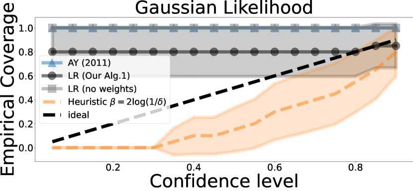
E.1 Calibration Plots

In Figure 3 we report the calibration of heuristics as well as other theoretically motivated works. The other theoretically motivated works are very pessimistic and are not appropriately calibrated. Note that one caveat of reporting calibration is that it is very much influenced by the data collection scheme in the sequential regime. In our case we use a bandit algorithm to collect the data. Arguably, in this setting, regret might be a better measure rather than looking at the calibration of the confidence sets. Additionally, the calibration depends on the true value ${\theta_{\star}}$ . We report the results for zero parameter and a random parameter from a unit ball. We also report results for i.i.d. data.

E.2 Baselines and Details

In the following section, we describe the baseline we used in the comparison. The details of parameters used in the experiments can be found in Table 2. As there is no explicit statement for sub-exponential variables, we give a formal derivation in Appendix F.

E.2.1 Sub-Exponential Random Variables: Confidence Sets

For this baseline, we will assume a linear model with additive sub-exponential noise, namely that there is $\theta_{*}\in\Theta$ such that $y_{t}=\langle\theta_{*},\,x_{t}\rangle+\eta_{t}$ , where $\eta_{t}$ is $(\nu,\gamma)$ -conditionally sub-exponential (Wainwright,, 2019). We let as usual

\mathbf{{V}}_{t}^{\nu^{-2};\lambda}=\sum_{s=1}^{t}\frac{x_{s}x_{s}^{\top}}{\nu^{2}}\lambda\mathbf{{I}}.

With this, one can prove the following time-uniform concentration result:

Proposition 3.

For any $k\in(0,1)$ , the following holds:

\mathbb{P}\left(\exists t\,:\,\lvert\lvert{\hat{{\theta}}}_{t}-\theta^{*}\rvert\rvert_{\mathbf{{V}}_{t}^{\nu^{-2};\lambda}}\geq\sqrt{\beta_{SE}}\right)\leq\delta,

where

\sqrt{\beta_{SE}}=\sqrt{\lambda}\lvert\lvert{\theta_{\star}}\rvert\rvert_{2}+\sqrt{\lambda}kB+\frac{d}{\sqrt{\lambda}kB}\log\left(\frac{1}{1-k}\right)+\frac{1}{\sqrt{\lambda}kB}\log\left(\frac{(\det(\mathbf{{V}}_{t}^{\nu^{-2};\lambda}))^{1/2}}{\delta\det(\sqrt{\lambda}\mathbf{{I}})}\right).

The proof is very similar to prior work Faury et al., (2020); Mutný and Krause, (2021), and can be found in Appendix F. This can readily be applied in the survival analysis (after a suitable transformation explained in the main paper) and Laplace noise experiments.

E.2.2 Poisson Heuristics

We implement two heuristics. One is a Bayesian formulation due to the Laplace method, and one is due to considerations in Mutný and Krause, (2021) of how to construct a valid confidence set using the Fisher information. The Laplace method creates an ellipsoidal confidence set using the second-order information evaluated at the penalized maximum likelihood estimator. Namely, the second derivative of the likelihood evaluated at the maximum penalized likelihood ${\hat{{\theta}}}_{t}$ is

\mathbf{{V}}_{\text{laplace}}=\sum_{s=1}^{t}\exp({\hat{{\theta}}}_{t}^{\top}x_{s})x_{s}x_{s}^{\top}.

We use this to define ellipsoidal confidence sets as $||{\hat{{\theta}}}_{t}-\theta||_{\mathbf{{V}}_{\text{laplace}}}^{2}\leq 2\log(1/\delta)$ . The other heuristic suggests using the worst-case parameter instead, namely

\mathbf{{V}}_{\text{mutny}}=\sum_{s=1}^{t}\exp(B)x_{s}x_{s}^{\top}.

This method would have provable coverage with a proper confidence parameter. Its derivation is beyond the scope of this paper.

E.2.3 NR (2021)

This method follows from Neiswanger and Ramdas, (2021). Per se, this method was not developed to be versatile in terms of likelihood but instead provides a confidence set on $f$ , even if it originates from a misspecified prior. Nevertheless, it provides a likelihood-aware confidence sequence that is anytime-valid and doesn’t employ worst-case parameters, and hence is a good benchmark for our analysis. The confidence sets are of the form

\{\theta\leavevmode\nobreak\ |\leavevmode\nobreak\ \log\mathcal{L}(\theta)\leq\log(1/\delta)+\log(p(\mathcal{D}))\},

where $\log(p(\mathcal{D}))$ is the current log-evidence of the data given the Gaussian prior. For more information, see Neiswanger and Ramdas, (2021).

Benchmark function	dim	$\|\mathcal{X}\|$	$\gamma$	$B$	$\lambda$	Gaussian/Laplace $\sigma$ / $b$
1D	1	$2^{6}$	0.06	4	1	0.15
Camelback	2	$10^{2}$	0.2	2	1	0.10

Table 2: Summary of experimental parameters

E.3 Additive Models

We implemented two likelihoods, namely Gaussian and Laplace. We implemented the discretization of the domain $|\mathcal{X}|$ , and in the implementation we used Nystrom features defined on $|\mathcal{X}|$ providing the exact representation of the RKHS on the $\mathcal{X}$ , The points were chosen to be on a uniform grid. Notice that for the regularized estimator, we chose the rule of thumb $\lambda=1/B$ as is motivated in (Mutný and Krause,, 2022).

The laplace parameter was picked as $b=0.15$ likewise. Note that Laplace distribution is sub-exponential with parameters $(b,2b^{2})$ . We use $1/\sigma^{2}$ or $1/b$ respectively for the value $L$ . Strictly speaking, the Laplace likelihood is not smooth, but a smoothed objective would most likely inherit a value depending on $b$ . As we maintain coverage with any choice of weighting, we do not risk invalidity by using a heuristic choice for $L$ .

E.4 Survival Analysis

We implemented the method exactly as specified, using the Weibull likelihood with parameter $p=2$ . Upon log-transformation, the Gumbel distribution is sub-exponential. To determine the parameter, consider the moment-generating function of the Gumbel distribution ( $\beta=1/p$ in the canonical parameterization):

\mathop{{}\mathbb{E}}[e^{X}t]=\Gamma(1-t/2)\exp(t)\leq\exp(t^{2}/2)\quad\text{for}\quad t<1/2,

hence, the sub-exponentiality parameter is $1$ , and we can use the above sub-exponential confidence sets with value $b=1$ . For the likelihood ratio code, we used $L=\exp(B)$ , as this is the leading term of the Hessian of log-likelihood. The function is not smooth everywhere, but on a bounded domain, this turns out to be an appropriate scaling.

E.5 Poisson Bandits

In this case, we implemented a bandit game, where we used the parametrization $r_{\theta}(x)\sim\text{Poisson}(\exp(-\theta^{\top}\Phi(x)))$ , where $\Phi(x)$ is the RKHS evaluation operator, and $\theta$ is the unknown value.

We used $L=\exp(B)$ , as this is the leading term of the Hessian of log-likelihood in this parametrization. The function is not smooth everywhere but on a bounded domain this is an appropriate scaling.

E.6 Additional Benchmark Functions

We focus on an additional baseline function: Camelback in 2D, a standard BO benchmark function. The results can be see in Figure 4.

Appendix F Proof of Proposition 3

Define $S_{t}$ and the shorthand $\mathbf{{V}}_{t}$

S_{t}=\sum_{s=1}^{t}\eta_{s}\frac{x_{s}}{\nu^{2}}\quad\text{and}\quad\mathbf{{V}}_{t}:=\mathbf{{V}}^{\nu^{-2};\lambda}_{t}=\sum_{s=1}^{t}\frac{x_{s}x_{s}^{\top}}{\nu^{2}}+\lambda\mathbf{{I}}.

and the parametrized process

\mathcal{M}_{t}(x)=\exp(\langle x,\,S_{t}\rangle-\frac{1}{2}\lvert\lvert x\rvert\rvert_{\mathbf{{V}}_{t}}^{2}).

Lemma 13.

If $\eta_{t}$ is $(\nu,\gamma)$ -conditionally sub-Exponential, then $\mathcal{M}_{t}(x)$ is a super-martingale on the ball $\{x\in\mathbb{R}^{d}\,|\,\lvert\lvert x\rvert\rvert_{2}\leq\frac{\nu^{2}}{\gamma}\}$ with $\mathcal{M}_{0}(x)\leq 1.$

Note that for $\gamma\rightarrow 0$ (sub-Gaussian case), this recovers Lemma 20.2. in Lattimore and Szepesvári, (2020).

Proof.

It is easy to observe that for any $x$ , we have

\exp\left(S_{0}^{\top}x-\frac{1}{2}\lvert\lvert x\rvert\rvert_{\mathbf{{V}}_{0}}^{2}\right)=\exp\left(-\frac{1}{2}\lvert\lvert x\rvert\rvert_{\lambda\mathbf{{I}}}^{2}\right)\leq 1.

For the first part, we can write

	$\displaystyle\mathop{{}\mathbb{E}}[\mathcal{M}_{t}(x)\|\mathcal{F}_{t-1}]$	$\displaystyle=\mathop{{}\mathbb{E}}[\exp(\langle x,\,S_{t}\rangle-\frac{1}{2}\lvert\lvert x\rvert\rvert_{\mathbf{{V}}_{t}}^{2})\,\|\,\mathcal{F}_{t-1}]$
		$\displaystyle=\mathop{{}\mathbb{E}}[\exp(\langle x,\,S_{t-1}\rangle-\frac{1}{2}\lvert\lvert x\rvert\rvert_{\mathbf{{V}}_{t-1}}^{2})\exp(\frac{1}{\nu^{2}}\langle x,\,\eta_{t}x_{t}\rangle-\frac{1}{2\nu^{2}}\lvert\lvert x\rvert\rvert^{2}_{x_{t}x_{t}^{\top}})\,\|\,\mathcal{F}_{t-1}]$
		$\displaystyle=\mathcal{M}_{t-1}(x)\mathop{{}\mathbb{E}}[\exp(\frac{1}{\nu^{2}}\eta_{t}\langle x,\,x_{t}\rangle)\,\|\,\mathcal{F}_{t-1}]\exp(-\frac{1}{2\nu^{2}}\lvert\lvert x\rvert\rvert_{x_{t}x_{t}^{\top}}^{2}),$

where in the last step we use that $x_{t}$ is $\mathcal{F}_{t-1}$ -measurable. Now, as long as $\frac{1}{\nu^{2}}\lvert\langle x,\,x_{s}\rangle\rvert\leq\frac{1}{\gamma}$ , we can apply our definition of conditional sub-Exponential noise to bound

\mathop{{}\mathbb{E}}[\exp(\eta_{t}\frac{1}{\nu^{2}}\langle x,\,x_{t}\rangle)]\leq\exp\left(\frac{(\langle x,\,x_{t}\rangle)^{2}\nu^{2}}{2\nu^{4}}\right)\leq\exp\left(\frac{\lvert\lvert x\rvert\rvert_{x_{t}x_{t}^{\top}}^{2}}{2\nu^{2}}\right).

From this we directly conclude

\mathop{{}\mathbb{E}}[\mathcal{M}_{t}(x)|\mathcal{F}_{t-1}]\leq\mathcal{M}_{t-1}(x).

By Cauchy-Schwarz, a sufficient condition is $\lvert\lvert x\rvert\rvert_{2}\leq\frac{\nu^{2}}{\gamma}$ as this implies (with our assumptions on the actions)

\lvert\langle x,\,x_{t}\rangle\rvert\leq\lvert\lvert x\rvert\rvert_{2}\lvert\lvert x_{t}\rvert\rvert_{2}\leq\lvert\lvert x\rvert\rvert_{2}\leq\frac{\nu^{2}}{\gamma}.

∎

In the following, will use this result to prove any-time confidence estimates for the parameter $\theta$ using the technique of pseudo-maximization, closely following Mutný and Krause, (2021).

Recall that $\mathcal{M}_{t}(x)$ is defined on the ball of radius $\frac{\nu^{2}}{\gamma L}$ . This allows us some freedom in choosing the radius of the ball on which we integrate. In particular, let $K$ be this radius. While we need $K\leq\frac{\nu^{2}}{\gamma L}$ , we can make $K$ larger by choosing larger $\nu^{2}$ (increasing $\nu^{2}$ only makes the set of noise distributions larger).

Ultimately, we wish to bound (following Lattimore and Szepesvári, (2020))

	$\displaystyle\lvert\lvert{\hat{{\theta}}}_{t}-\theta^{*}\rvert\rvert_{\mathbf{{V}}_{t}}$	$\displaystyle=\lvert\lvert\mathbf{{V}}_{t}^{-1}X_{1:t}(X_{1:t}{\theta_{\star}}+\eta_{1:t})-{\theta_{\star}}\rvert\rvert_{\mathbf{{V}}_{t}}$
		$\displaystyle=\lvert\lvert\mathbf{{V}}_{t}^{-1}X_{1:t}X_{1:t}{\theta_{\star}}-{\theta_{\star}}+\mathbf{{V}}_{t}^{-1}S_{t}\rvert\rvert_{\mathbf{{V}}_{t}}$
		$\displaystyle\leq\lvert\lvert S_{t}\rvert\rvert_{\mathbf{{V}}_{t}^{-1}}+\sqrt{\lambda}\lvert\lvert{\theta_{\star}}\rvert\rvert_{2}.$

We can not control the second term, so we focus on the first: the self-normalized residuals. Via fenchel duality, one can motivate that the right object to study is the supremum of the martingale $\mathcal{M}_{t}(x)$ over all $x\in\mathbb{R}$ .⁴⁴4But that is in our case ill-defined. Define $\tilde{M}_{t}$ to be the martingale $\mathcal{M}_{t}$ from above but with $\lambda=0$ , i.e. no regularisation term. Similarly, let $\tilde{\mathbf{{V}}}_{t}=\mathbf{{V}}_{t}-\lambda\mathbf{{I}}$ be the design matrix without the regularisation term. Slightly counterintuitively, we will study

\bar{M}_{t}=\int_{\lvert\lvert x\rvert\rvert_{2}\leq K}\tilde{M}_{t}(x)\mathrm{{d}}h(x),

where $h$ is the probability density function of a truncated normal distribution with inverse variance $\lambda$ , that is with covariance matrix $\frac{1}{\lambda}\mathbf{{I}}$ . By Lemma 20.3 in Lattimore and Szepesvári, (2020), $\bar{M}_{t}$ is also a super-martingale with $\bar{M}_{0}\leq 1$ . Then we have

	$\displaystyle\bar{M}_{t}$	$\displaystyle=\frac{1}{N(h)}\int_{\lvert\lvert x\rvert\rvert_{2}\leq K}\exp\left(x^{\top}S_{t}-\frac{1}{2}\lvert\lvert x\rvert\rvert_{\tilde{\mathbf{{V}}}_{t}}^{2}\right)\exp\left(-\frac{1}{2}x^{\top}\lambda\mathbf{{I}}x\right)\mathrm{{d}}x$
		$\displaystyle=\frac{1}{N(h)}\int_{\lvert\lvert x\rvert\rvert_{2}\leq K}\exp\left(x^{\top}S_{t}-\frac{1}{2}\lvert\lvert x\rvert\rvert_{\mathbf{{V}}_{t}}^{2}\right)\mathrm{{d}}x.$

We will define the shorthand $f_{t}(x)=x^{\top}S_{t}-\frac{1}{2}x^{\top}\mathbf{{V}}_{t}x=f_{t}(x^{*})+\nabla f_{t}(x^{*})^{\top}(x-x^{*})-\frac{1}{2}(x-x^{*})^{\top}\mathbf{{V}}_{t}(x-x^{*})$ (by Taylor’s theorem), where $x^{*}=\arg\max_{\lvert\lvert x\rvert\rvert\leq kK}f_{t}(x)$ , $k\in(0,1)$ will be chosen later. We can lower bound $\bar{M}_{t}$ by

$\displaystyle\bar{M}_{t}$	$\displaystyle=\frac{1}{N(h)}\int_{\lvert\lvert x\rvert\rvert_{2}\leq K}\exp\left(x^{\top}S_{t}-\frac{1}{2}\lvert\lvert x\rvert\rvert_{\mathbf{{V}}_{t}}^{2}\right)\mathrm{{d}}x$
	$\displaystyle=\frac{\exp(f_{t}(x^{}))}{N(h)}\int_{\lvert\lvert x\rvert\rvert_{2}\leq K}\exp\left(\nabla f_{t}(x^{})^{\top}(x-x^{})-\frac{1}{2}(x-x^{})^{\top}\mathbf{{V}}_{t}(x-x^{*})\right)\mathrm{{d}}x$
	$\displaystyle=\frac{\exp(f_{t}(x^{}))}{N(h)}\int_{\lvert\lvert y+x^{}\rvert\rvert_{2}\leq K}\exp\left(\nabla f_{t}(x^{*})^{\top}y-\frac{1}{2}y^{\top}\mathbf{{V}}_{t}y\right)\mathrm{{d}}y$	(34)
	$\displaystyle\geq\frac{\exp(f_{t}(x^{}))}{N(h)}\int_{\lvert\lvert y\rvert\rvert_{2}\leq(1-k)K}\exp\left(\nabla f_{t}(x^{})^{\top}y-\frac{1}{2}y^{\top}\mathbf{{V}}_{t}y\right)\mathrm{{d}}y$	(35)
	$\displaystyle=\frac{\exp(f_{t}(x^{}))}{N(h)}\int_{\lvert\lvert y\rvert\rvert_{2}\leq(1-k)K}\exp\left(\nabla f_{t}(x^{})^{\top}y\right)\exp\left(-\frac{1}{2}y^{\top}\mathbf{{V}}_{t}y\right)\mathrm{{d}}y$
	$\displaystyle=\frac{\exp(f_{t}(x^{}))N(g)}{N(h)}\mathop{{}\mathbb{E}}_{y\sim g}\left[\exp\left(\nabla f_{t}(x^{})^{\top}y\right)\right]$
	$\displaystyle\geq\frac{\exp(f_{t}(x^{}))N(g)}{N(h)}\exp\left(\mathop{{}\mathbb{E}}_{y\sim g}[\nabla f_{t}(x^{})^{\top}y]\right)$	(36)
	$\displaystyle=\frac{\exp(f_{t}(x^{*}))N(g)}{N(h)}.$

where in step (34) we used the change of variables $x=y+x^{*}$ . In (35) we use that if $\lvert\lvert y\rvert\rvert_{2}\leq(1-k)K$ , then $\lvert\lvert x^{*}+y\rvert\rvert_{2}\leq\lvert\lvert x^{*}\rvert\rvert_{2}+\lvert\lvert y\rvert\rvert_{2}\leq(1-k)K+kK=K$ . Finally, in (36), we used Jensen’s inequality. The last inequality follows from symmetry. Note that we implicitly defined $g$ to be a truncated normal distribution with covariance matrix $\mathbf{{V}}_{t}^{-1}$ on the ball of radius $(1-k)K$ .

This puts us in a position to put Ville’s inequality to good use:

	$\displaystyle\delta$	$\displaystyle\geq\mathbb{P}\left(\exists t\,:\,\log(\bar{M_{t}})\geq\log(1/\delta)\right)$
		$\displaystyle\geq\mathbb{P}\left(\exists t\,:\,f_{t}(x^{*})+\log\left(\frac{N(g)}{N(h)}\right)\geq\log(1/\delta)\right)$
		$\displaystyle\geq\mathbb{P}\left(\exists t\,:\,f_{t}(x^{*})\geq\log\left(\frac{N(h)}{N(g)\delta}\right)\right).$

We now wish to recover $\lvert\lvert S_{t}\rvert\rvert_{\mathbf{{V}}_{t}}$ . Recall the definition of $f_{t}(x^{*})$ as the maximum over all $x$ in a ball of radius $kK$ . Consequently, we can choose $x=\frac{\mathbf{{V}}_{t}^{-1}S_{t}}{\lvert\lvert S_{t}\rvert\rvert_{\mathbf{{V}}_{t}^{-1}}}\sqrt{\lambda}kK$ , which has norm bounded by $kK$ . We have

f_{t}(x^{*})\geq f_{t}\left(\frac{\mathbf{{V}}_{t}^{-1}S_{t}}{\lvert\lvert S_{t}\rvert\rvert_{\mathbf{{V}}_{t}^{-1}}}\sqrt{\lambda}kK\right)=\lvert\lvert S_{t}\rvert\rvert_{\mathbf{{V}}_{t}^{-1}}\sqrt{\lambda}kK-\lambda k^{2}K^{2},

which immediately yields

\displaystyle\mathbb{P}\left(\lvert\lvert S_{t}\rvert\rvert_{\mathbf{{V}}_{t}^{-1}}\geq\sqrt{\lambda}kK+\frac{1}{\sqrt{\lambda}kK}\log\left(\frac{N(h)}{N(g)\delta}\right)\right)\leq\delta.

The only thing that remains is bounding $\log\left(\frac{N(h)}{N(g)}\right)$ .

We give the following Lemma that is a slightly generalized version of Mutný and Krause, (2021) and originally inspired by Faury et al., (2020).

Lemma 14.

The normalizing constants satisfy

\log\left(\frac{N(h)}{N(g)}\right)\leq d\log\left(\frac{1}{1-k}\right)+\log\left(\frac{(\det(\mathbf{{V}}_{t}))^{1/2}}{\det(\sqrt{\lambda}\mathbf{{I}})}\right).

We can use the bound from Lemma 14 to conclude that

\displaystyle\mathbb{P}\left(\lvert\lvert S_{t}\rvert\rvert_{\mathbf{{V}}_{t}^{-1}}\geq\sqrt{\lambda}kK+\frac{d}{\sqrt{\lambda}kK}\log\left(\frac{1}{1-k}\right)+\frac{1}{\sqrt{\lambda}kK}\log\left(\frac{(\det(\mathbf{{V}}_{t}))^{1/2}}{\delta\det(\sqrt{\lambda}\mathbf{{I}})}\right)\right)\leq\delta.

We stated earlier that

\lvert\lvert{\hat{{\theta}}}_{t}-\theta^{*}\rvert\rvert_{\mathbf{{V}}_{t}}\leq\lvert\lvert S_{t}\rvert\rvert_{\mathbf{{V}}_{t}^{-1}}+\sqrt{\lambda}\lvert\lvert{\theta_{\star}}\rvert\rvert_{2}.

Combining this with our analysis, we get the Proposition 3.

We may now choose the parameters $k$ , $K$ and $\lambda$ . Note that to get sub-Gaussian rates as in Abbasi-Yadkori, one needs to pick a regularization parameter of the order of $\lambda=d\log(T)$ .

Proof of Lemma 14

We give a proof of the Lemma for completeness, and because the additional generality makes for a slightly different proof, even though the bound stays the same.

Proof.

We have

	$\displaystyle N(h)$	$\displaystyle=\int_{\lvert\lvert x\rvert\rvert_{2}\leq K}\exp(-\lambda\lvert\lvert x\rvert\rvert_{2}^{2})\mathrm{d}x$
		$\displaystyle=\frac{1}{\lvert\det(\sqrt{2\lambda}\mathbf{{I}})\rvert}\int_{\lvert\lvert x\rvert\rvert_{2}\leq K}\exp\left(-\frac{1}{2}\lvert\lvert\sqrt{2\lambda}x\rvert\rvert_{2}^{2}\right)\lvert\det(\sqrt{2\lambda}\mathbf{{I}})\rvert\mathrm{d}x$
		$\displaystyle=\frac{1}{\lvert\det(\sqrt{2\lambda}\mathbf{{I}})\rvert}\int_{\lvert\lvert x\rvert\rvert_{2}\leq\sqrt{2\lambda}K}\exp\left(-\frac{1}{2}\lvert\lvert x\rvert\rvert_{2}^{2}\right)\mathrm{d}x.$

Further we have

	$\displaystyle N(g)$	$\displaystyle=\int_{\lvert\lvert x\rvert\rvert_{2}\leq(1-k)K}\exp(-\frac{1}{2}x^{\top}\mathbf{{V}}_{t}x)\mathrm{d}x$
		$\displaystyle=\frac{1}{\lvert\det(\mathbf{{V}}_{t}^{1/2})\rvert}\int_{\lvert\lvert x\rvert\rvert_{2}\leq(1-k)K}\exp(-\frac{1}{2}\lvert\lvert\mathbf{{V}}_{t}^{1/2}x\rvert\rvert_{2}^{2})\lvert\det(\mathbf{{V}}_{t}^{1/2})\rvert\mathrm{d}x$
		$\displaystyle=\frac{1}{\lvert\det(\mathbf{{V}}_{t}^{1/2})\rvert}\int_{S}\exp(-\frac{1}{2}\lvert\lvert x\rvert\rvert_{2}^{2})\mathrm{d}x,$

where $S=\{\mathbf{{V}}_{t}^{1/2}x\,|\,\lvert\lvert x\rvert\rvert\leq(1-k)K\}=\{x\,|\,\lvert\lvert\mathbf{{V}}_{t}^{-1/2}x\rvert\rvert\leq(1-k)K\}=\{x\,|\,x^{\top}\mathbf{{V}}_{t}^{-1}x\leq(1-k)K\}$ . Note that $\mathbf{{V}}_{t}\succeq\lambda\mathbf{{I}}$ and so $\mathbf{{V}}_{t}^{-1}\preceq\frac{1}{\lambda}\mathbf{{I}}$ . Therefore if $\lvert\lvert x\rvert\rvert_{2}^{2}\leq(1-k)K\sqrt{\lambda}$ , we have

\sqrt{x^{\top}\mathbf{{V}}_{t}^{-1}x}\leq\frac{1}{\sqrt{\lambda}}\lvert\lvert x\rvert\rvert_{2}\leq(1-k)K\implies x\in S.

Thus $\{x\,|\,\lvert\lvert x\rvert\rvert_{2}\leq(1-k)\sqrt{\lambda}K\}\subseteq S$ and

N(g)\geq\frac{1}{\lvert\det(\mathbf{{V}}_{t}^{1/2})\rvert}\int_{\lvert\lvert x\rvert\rvert_{2}\leq(1-k)\sqrt{\lambda}K}\exp(-\frac{1}{2}\lvert\lvert x\rvert\rvert_{2}^{2})\mathrm{d}x.

We may therefore bound

\frac{N(g)}{N(h)}\leq\frac{(\det\mathbf{{V}}_{t})^{1/2}}{(\det\sqrt{2\lambda}\mathbf{{I}})}\frac{\int_{\lvert\lvert x\rvert\rvert_{2}\leq\sqrt{2\lambda}K}\exp\left(-\frac{1}{2}\lvert\lvert x\rvert\rvert_{2}^{2}\right)\mathrm{d}x}{\int_{\lvert\lvert x\rvert\rvert_{2}\leq(1-k)\sqrt{\lambda}K}\exp(-\frac{1}{2}\lvert\lvert x\rvert\rvert_{2}^{2})\mathrm{d}x}.

By a rather crude bound (as $1-k\leq\sqrt{2}$ in any case) we get

		$\displaystyle\frac{\int_{\lvert\lvert x\rvert\rvert_{2}\leq\sqrt{2\lambda}K}\exp\left(-\frac{1}{2}\lvert\lvert x\rvert\rvert_{2}^{2}\right)\mathrm{d}x}{\int_{\lvert\lvert x\rvert\rvert_{2}(1-k)\sqrt{\lambda}K}\exp(-\frac{1}{2}\lvert\lvert x\rvert\rvert_{2}^{2})\mathrm{d}x}$
	$\displaystyle\leq\,\,$	$\displaystyle\frac{\int_{\lvert\lvert x\rvert\rvert_{2}\leq(1-k)\sqrt{\lambda}K}\exp\left(-\frac{1}{2}\lvert\lvert x\rvert\rvert_{2}^{2}\right)\mathrm{d}x+\int_{(1-k)\sqrt{\lambda}K\leq\lvert\lvert x\rvert\rvert_{2}\leq\sqrt{2\lambda}K}\exp\left(-\frac{1}{2}\lvert\lvert x\rvert\rvert_{2}^{2}\right)\mathrm{d}x}{\int_{\lvert\lvert x\rvert\rvert_{2}\leq(1-k)\sqrt{\lambda}K}\exp(-\frac{1}{2}\lvert\lvert x\rvert\rvert_{2}^{2})\mathrm{d}x}$
	$\displaystyle=\,\,$	$\displaystyle 1+\frac{\int_{(1-k)\sqrt{\lambda}K\leq\lvert\lvert x\rvert\rvert_{2}\leq\sqrt{2\lambda}K}\exp\left(-\frac{1}{2}\lvert\lvert x\rvert\rvert_{2}^{2}\right)\mathrm{d}x}{\int_{\lvert\lvert x\rvert\rvert_{2}\leq(1-k)\sqrt{\lambda}K}\exp(-\frac{1}{2}\lvert\lvert x\rvert\rvert_{2}^{2})\mathrm{d}x}$
	$\displaystyle\leq\,\,$	$\displaystyle 1+\frac{\exp\left(-\frac{1}{2}(1-k)^{2}\lambda K^{2}\right)}{\exp\left(-\frac{1}{2}(1-k)^{2}\lambda K^{2}\right)}\frac{\int_{(1-k)\sqrt{\lambda}K\leq\lvert\lvert x\rvert\rvert_{2}\leq\sqrt{2\lambda}K}\mathrm{d}x}{\int_{\lvert\lvert x\rvert\rvert_{2}\leq(1-k)\sqrt{\lambda}K}\mathrm{d}x}$
	$\displaystyle=\,\,$	$\displaystyle 1+\frac{\mathrm{vol}_{d}(\sqrt{2\lambda}K)-\mathrm{vol}_{d}((1-k)\sqrt{\lambda}K)}{\mathrm{vol}_{d}((1-k)\sqrt{\lambda}K)}$
	$\displaystyle=\,\,$	$\displaystyle\frac{\mathrm{vol}_{d}(\sqrt{2\lambda}K)}{\mathrm{vol}_{d}((1-k)\sqrt{\lambda}K)}$
	$\displaystyle=\,\,$	$\displaystyle(1-k)^{-d}\sqrt{2}^{d}.$

We can put this together to obtain

\frac{N(h)}{N(g)}\leq(1-k)^{-d}\sqrt{2}^{d}\frac{(\det(\mathbf{{V}}_{t}))^{1/2}}{\det(\sqrt{2\lambda}\mathbf{{I}})}=(1-k)^{-d}\frac{(\det(\mathbf{{V}}_{t}))^{1/2}}{\det(\sqrt{\lambda}\mathbf{{I}})}.

∎

	$\displaystyle\mathop{{}\mathbb{E}}[\mathcal{M}_{t}(x)\|\mathcal{F}_{t-1}]$	$\displaystyle=\mathop{{}\mathbb{E}}[\exp(\langle x,\,S_{t}\rangle-\frac{1}{2}\lvert\lvert x\rvert\rvert_{\mathbf{{V}}_{t}}^{2})\,\|\,\mathcal{F}_{t-1}]$
		$\displaystyle=\mathop{{}\mathbb{E}}[\exp(\langle x,\,S_{t-1}\rangle-\frac{1}{2}\lvert\lvert x\rvert\rvert_{\mathbf{{V}}_{t-1}}^{2})\exp(\frac{1}{\nu^{2}}\langle x,\,\eta_{t}x_{t}\rangle-\frac{1}{2\nu^{2}}\lvert\lvert x\rvert\rvert^{2}_{x_{t}x_{t}^{\top}})\,\|\,\mathcal{F}_{t-1}]$
		$\displaystyle=\mathcal{M}_{t-1}(x)\mathop{{}\mathbb{E}}[\exp(\frac{1}{\nu^{2}}\eta_{t}\langle x,\,x_{t}\rangle)\,\|\,\mathcal{F}_{t-1}]\exp(-\frac{1}{2\nu^{2}}\lvert\lvert x\rvert\rvert_{x_{t}x_{t}^{\top}}^{2}),$

Likelihood Ratio Confidence Sets for Sequential Decision Making

Abstract

1 Introduction

Contributions

2 The Likelihood Method

Theorem 1.

2.1 The Estimator Sequence Game

Online Prediction Game

Online Optimization Algorithms

2.2 Adaptive Reweighting: Choosing the Right Loss

Intuition

Bias estimation

Theorem 2 (Bias estimate).

3 Theory: Linear Models

3.1 Generalized Linear Models

Assumption 1.

3.2 Geometry and Concentration

Theorem 3.

3.3 Online Optimization in GLMs: Follow the Regularized Leader

Theorem 4.

Regret, Weighting and Estimation Bias

Theorem 5.

4 Application: Linear and Kernelized Bandits

Extension to RKHS

4.1 Instantiation of the Theory for Linear Bandits

Theorem 6.

4.2 Experimental Evaluation

Additive Noise Models

Poisson Bandits

Survival Analysis

5 Related Work and Conclusion

Related Work

Conclusion

Acknowledgments and Disclosure of Funding

References

Appendix A Proofs of Theorem 1 and 2

A.1 GLM Families

A.2 Proof of Theorem 1 (Coverage)

Proof.

A.3 Proof of Theorem 2 (Bias)

Lemma 1 (Convexity: Gradient).

Proof.

Proof of Theorem 2.

GLM models

Appendix B Proof of Theorem 3 (Bregman Ball Confidence Set)

Proof sketch

B.1 Technical Lemmas

Definition 1.

Lemma 2.

Lemma 3.

Notational Shorthands

Proposition 1 (Theorem 7 in Chowdhury et al., (2022)).

Lemma 4.

B.2 Proof of Theorem 3

B.3 Proof of Technical Lemmas

Proof.

Lemma 5.

Proof.

Proof.

Appendix C FTRL Results: Proofs

C.1 Technical Lemmas I: Exponential Families

Lemma 6 (MGF for Exponential family).

Proof.

C.2 Technical Lemmas II: Elliptical Potential Lemma

Lemma 7 (Lemma 11 in Hazan et al., (2006)).

Corollary 1.

Proof.

C.3 Technical Lemmas III: Supermartingales

Lemma 8 (Martingale Increment).

Proof.

Lemma 9.

Proof.

Lemma 10.

Proof.

Lemma 11 (Weighting Reduction).

Proof.

C.4 FTRL Proof: the Unweighted Case

Proof of Theorem 4 (first part).

C.5 FTRL Analysis: the Weighted Case (Vovk-Azoury-Warmuth Forecaster)

Proof.

Likelihood Ratio Confidence Sets for
Sequential Decision Making