LightWeather: Harnessing Absolute Positional Encoding for Efficient and Scalable Global Weather Forecasting
Abstract
Recently, Transformers have gained traction in weather forecasting for their capability to capture long-term spatial-temporal correlations. However, their complex architectures result in large parameter counts and extended training times, limiting their practical application and scalability to global-scale forecasting. This paper aims to explore the key factor for accurate weather forecasting and design more efficient solutions. Interestingly, our empirical findings reveal that absolute positional encoding is what really works in Transformer-based weather forecasting models, which can explicitly model the spatial-temporal correlations even without attention mechanisms. We theoretically prove that its effectiveness stems from the integration of geographical coordinates and real-world time features, which are intrinsically related to the dynamics of weather. Based on this, we propose LightWeather, a lightweight and effective model for station-based global weather forecasting. We employ absolute positional encoding and a simple MLP in place of other components of Transformer. With under 30k parameters and less than one hour of training time, LightWeather achieves state-of-the-art performance on global weather datasets compared to other advanced DL methods. The results underscore the superiority of integrating spatial-temporal knowledge over complex architectures, providing novel insights for DL in weather forecasting.
Introduction
Accurate weather forecasting is of great significance in a wide variety of domains such as agriculture, transportation, energy, and economics. In the past decades, there was an exponential growth in the number of automatic weather stations, which play a pivotal role in modern meteorology (Sose and Sayyad 2016). They are cost-effective for applications (Bernardes et al. 2023; Tenzin et al. 2017) and can be flexibly deployed to almost anywhere around the world, collecting meteorological data at any desired resolution.
With the development of deep learning (DL), studies have embarked on exploring DL approaches for weather forecasting. The goal of data-driven DL methods is to fully leverage the historical data to enhance the accuracy of forecasting (Schultz et al. 2021). The weather stations around the world are ideally positioned to provide a substantial amount of data for DL methods. However, the observations of worldwide stations exhibit intricate spatial-temporal patterns that vary across regions and periods, posing challenge for global-scale weather forecasting (Wu et al. 2023b).

Recently, Transformers have become increasingly popular in weather forecasting due to their capability to capture long-term spatial-temporal correlations. When confronting the challenge of global-scale forecasting, Transformer-based methods employ more sophisticated architectures, leading to hundreds of millions of parameters and multiple days of training time. In the era of large model (LM), this phenomenon become particularly evident. Such expenses limit their scalability to large-scale stations and restrict their application in practical scenarios (Deng et al. 2024).
Despite the complexity of these architectures, we observe that the resulting improvements in performance are, in fact, quite limited. This motivates us to rethink the bottleneck of station-based weather forecasting and further design a model as effective as Transformer-based methods but more efficient and scalable. For this purpose, we delve deeper into the architecture of Transformer-based weather forecasting models and obtain an interesting conclusion: absolute positional encoding is what really works in Transformer-based weather forecasting models, and the reason lies in the principle of atmospheric dynamics.
Positional encoding is widely regarded as an adjunct to permutation-invariant attention mechanisms, providing positional information of tokens in sequence (Vaswani et al. 2017). However, we empirically find that absolute positional encoding can inherently model the spatial-temporal correlations of worldwide stations, even in the absence of attention mechanisms, by integrating 3D geographical coordinates (i.e., latitude, longitude, and elevation) and real-world temporal knowledge.
Furthermore, we will theoretically elucidate why absolute positional encoding is pivotal by applying principles of atmospheric dynamics. In the global weather system, the evolution of atmospheric states is closely related to absolute spatial and temporal conditions, resulting in complex correlations. Absolute positional encoding enables the model to explicitly capture these correlations rather than blind guessing, which is the key bottleneck in model performance.
Based on the aforementioned findings, we propose LightWeather, a lightweight and effective weather forecasting model that can collaboratively forecast for worldwide weather stations. It utilizes the absolute positional encoding and replaces the main components of Transformer with an MLP as encoder. Benefiting from its simplicity, LightWeather significantly surpass the current Transformer-based models in terms of efficiency. Despite its efficiency, LightWeather also achieves state-of-the-art forecasting performance among 13 baselines. Figure 1 visualizes LightWeather’s lead in both efficiency and performance. Moreover, it is worth noting that the computational complexity of LightWeather grows linearly with the increase of the number of stations and the parameter count is independent of . Therefore, LightWeather can perfectly scale to the fine-grained data with a larger .
Our contributions can be summarized as follows:
-
•
We innovatively highlight the importance of the absolute positional encoding in Transformer-based weather forecasting model. Even in the absence of attention mechanisms, it helps model to explicitly capture spatial-temporal correlations by introducing spatial and temporal knowledge into the model.
-
•
We propose LightWeather, a lightweight and effective weather forecasting model. We utilize the absolute positional encoding and replace the main components of Transformer with an MLP. The concise structure endows it with high efficiency and scalability to fine-grained data.
-
•
LightWeather achieves collaborative forecasting for worldwide stations with state-of-the-art performances. Experiments on 5 datasets show that LightWeather can outperform 13 mainstream baselines.
Related Works
DL Methods for Station-based Weather Prediction
Although there has been a great success of radar- or reanalysis-based DL methods (Bi et al. 2023; Lam et al. 2023; Chen et al. 2023), they can only process gridded data and are incompatible with station-based forecasting.
For station-based forecasting, spatial-temporal graph neural networks (STGNNs) are proved to be effective in modeling spatial-temporal patterns of weather data (Lin et al. 2022; Ni, Wang, and Fang 2022), but most of them only provide short-term forecasting (i.e., 6 or 12 steps), which limits their applicability.
Recently, Transformer-based approaches have gained more popularity for their capability of capturing long-term spatial-temporal correlations. For instance, MGSFformer (Yu et al. 2024a) and MRIformer (Yu et al. 2024b) employ attention mechanisms to capture correlations from multi-resolution data obtained through down sampling. However, attention mechanisms take quadratic computational complexity for both spatial and temporal correlation modeling, which is unaffordable in global-scale forecasting.
Several studies attempted to enhance the efficiency of attention mechanisms. Typically, AirFormer (Liang et al. 2023) restricts attention to focusing only on local information. Corrformer (Wu et al. 2023b) employs a more efficient multi-correlation mechanism to supplant attention mechanisms. Nevertheless, these optimizations came with a greater amount of computation and parameter, resulting in limited improvements in efficiency.
Studies of the effectiveness of Transformers
The effectiveness of Transformers has been thoroughly discussed in the fields of computer vision (CV) (Yu et al. 2022; Lin et al. 2024) and natural language processing (NLP) (Bian et al. 2021). In time series forecasting (TSF), LSTF-Linear (Zeng et al. 2023) pioneered the exploration and outperformed a variety of Transformer-based methods with a linear model. Shao et al. (2023) posited that Transformer-based models face over-fitting problem on specific datasets. MTS-Mixers (Li et al. 2023) and MEAformer (Huang et al. 2024) further questioned the necessity of attention mechanisms in Transformers for TSF and replaced them with MLP-based information aggregations. These studies consider positional encoding as supplementary to attention mechanisms and consequently remove it along with attention mechanisms, yet none have recognized the importance of positional encoding.
Methodology

Preliminaries
Problem Formulation.
We consider weather stations and each station collects meteorological variables (e.g., temperature). Then the observed data at time can be denoted as . The 3D geographical coordinates of stations are organized as a matrix , which is naturally accessible in station-based forecasting. Given the historical observation of all stations from the past time steps and optional spatial and temporal information, we aim to learn a function to forecast the values of future time steps :
| (1) |
where is the historical data, and is the future data.
Overview of LightWeather
As illustrated in Figure 2, LightWeather consists of a data embedding layer, an absolute positional encoding layer, an MLP as encoder, and a regression layer. LightWeather replaces the redundant structures in Transformer-based models with a simple MLP, which greatly enhances the efficiency without compromising performance.
Data Embedding
Let be the historical time series of station and variable . The data embedding layer maps to the embedding in latent space:
| (2) |
where denotes a fully connected layer.
Absolute Positional Encoding
Absolute positional encoding injects information about the absolute position of the tokens in sequence, which is widely regarded as an adjunct to permutation-invariant attention mechanisms. However, we find it helpful to capture spatial-temporal correlations by introducing additional geographical and temporal knowledge into the model.
In our model, absolute positional encoding includes two parts: spatial encoding and temporal encoding.
Spatial Encoding.
Spatial encoding provides the geographical knowledge of stations to the model, which can explicitly model the spatial correlations among worldwide stations. Specifically, we encode the geographical coordinates of the station into latent space by a simple fully connected layer, thus spatial encoding can be denoted as:
| (3) |
where represents the coordinates of the station .
Temporal Encoding.
Temporal encoding provides real-world temporal knowledge to the model. We utilize three learnable embedding matrices , and to save the temporal encodings of all time steps (Shao et al. 2022). They represent the patterns of weather in three scales ( denotes hours in a day, denotes days in a month and denotes the months in a year), contributing to model the multi-scale temporal correlations of weather. We add them together with data embedding to obtain :
| (4) |
Encoder
We utilize a -layer MLP as encoder to learn the representation from the embedded data . The l-th MLP layer with residual connect can be denoted as:
| (5) |
where is the activation function and .
Regression Layer
We employ a linear layer to map the representation to the specified dimension, yielding the prediction .

Loss Function
We adopt Mean Absolute Error (MAE) as the loss function for LightWeather. MAE measures the discrepancy between the prediction and the ground truth by:
| (6) |
| Dataset | GlobalWind | GlobalTemp | Wind_CN | Temp_CN | Wind_US | |||||
|---|---|---|---|---|---|---|---|---|---|---|
| Metric | MSE | MAE | MSE | MAE | MSE | MAE | MSE | MAE | MSE | MAE |
| HI | 7.285 | 1.831 | 14.89 | 2.575 | 90.08 | 6.576 | 42.45 | 4.875 | 5.893 | 1.733 |
| ARIMA | 4.479 | 1.539 | 20.93 | 3.267 | 57.66 | 5.292 | 27.62 | 3.825 | 5.992 | 1.801 |
| Informer | 4.716 | 1.496 | 33.29 | 4.415 | 59.24 | 5.186 | 20.39 | 3.041 | 3.095 | 1.300 |
| FEDformer | 4.662 | 1.471 | 11.05 | 2.405 | 53.16 | 5.039 | 19.55 | 3.252 | 3.363 | 1.362 |
| DSformer | 4.028 | 1.347 | 9.544 | 2.057 | 51.36 | 4.923 | 21.33 | 3.301 | 3.266 | 1.305 |
| PatchTST | 3.891 | 1.332 | 9.795 | 2.062 | 51.33 | 4.932 | 23.11 | 3.426 | 3.220 | 1.324 |
| TimesNet | 4.724 | 1.459 | 11.81 | 2.327 | 51.27 | 4.899 | 20.21 | 3.203 | 3.294 | 1.312 |
| GPT4TS | 4.686 | 1.456 | 12.01 | 2.336 | 50.87 | 4.883 | 20.87 | 3.253 | 3.230 | 1.296 |
| Time-LLM | -* | -* | -* | -* | 56.34 | 5.079 | 30.40 | 4.189 | 4.044 | 1.497 |
| DLinear | 4.022 | 1.350 | 9.914 | 2.072 | 51.18 | 4.931 | 22.18 | 3.400 | 3.455 | 1.339 |
| AirFormer | 3.810 | 1.314 | 31.30 | 4.127 | 53.69 | 5.008 | 21.49 | 3.389 | 3.116 | 1.272 |
| Corrformer | 3.889 | 1.304 | 7.709 | 1.888 | 51.31 | 4.908 | 21.20 | 3.248 | 3.362 | 1.339 |
| MRIformer | 3.906 | 1.318 | 9.516 | 1.999 | 51.48 | 4.934 | 22.98 | 3.408 | 3.300 | 1.310 |
| LightWeather (ours) | 3.734 | 1.295 | 7.420 | 1.858 | 50.15 | 4.869 | 17.04 | 2.990 | 3.047 | 1.270 |
| 0.003 | 0.002 | 0.010 | 0.002 | 0.03 | 0.001 | 0.03 | 0.005 | 0.003 | 0.003 | |
-
*
Dashes denote the out-of-memory error.
Theoretical Analysis
In this part, we provide a theoretical analysis of LightWeather, focusing on its effectiveness and efficiency of spatial-temporal embedding.
Effectiveness of LightWeather.
The effectiveness of LightWeather lies in the fact that absolute positional encoding integrates geographical coordinates and real-world time features into the model, which are intrinsically linked to the evolution of atmospheric states in global weather system. Here we theoretically demonstrate this relationship.
Theorem 1.
Let be the longitude, latitude and elevation of a weather station and is a meteorological variable collected by the station, then the time evolution of is a function of and time :
| (7) |
Proof.
We provide the proof with zonal wind speed as an example; analogous methods can be applied to other meteorological variables.
According to the basic equations of atmospheric dynamics in spherical coordinates (Marchuk 2012), the zonal wind speed obeys the equation:
| (8) |
where , is pressure, is atmospheric density, is zonal friction force, and is geocentric distance.
The geocentric distance can be further denoted as , where is the radius of the earth and is the elevation. Since is a constant and , we have and we can approximate with .
It is possible to render the left side of the equation spatial-independent by rearranging terms:
| (9) |
Therefore, we have
| (10) |
∎
Considering the use of historical data spanning steps for prediction, it is not difficult to draw the corollary:
Corollary 1.1.
| (11) |
where is the historical data, and .
The detailed proof is provided in Appendix A.1. According to Eq. (11), we conclude that predictions for the future are bifurcated into two components: the fitting to historical observations and the modeling of the function , which represents the spatial-temporal correlations. When the scale is small, e.g., in single-station forecasting, even a simple linear model can achieve great performances (Zeng et al. 2023). However, as the scale expands to global level, modeling becomes the key bottleneck of forecasting.
The majority of prior models are designed to fit historical observations more accurately by employing increasingly complex structures. As shown in Figure 3 (a) (b), they simplistically regard as a function of historical values, and the complex structures may lead to over-fitting of it. In comparison, LightWeather can explicitly model with introduced by absolute positional encoding, as shown in Figure 3 (c), thereby enhancing the predictive performance.
Efficiency of LightWeather.
We theoretically analyze the efficiency of LightWeather from the perspectives of parameter volume and computational complexity.
Theorem 2.
The total number of parameters required for the LightWeather is .
The proof is provided in Appendix A.2. According to Theorem 2, we conclude that the parameter count of LightWeather is independent of the number of stations . In addition, the computational complexity of LightWeather grows linearly as the increase of . In canonical spatial correlation modeling methods (Wu et al. 2019), it will cause quadratic complexity and linear increase of parameters with respect to , which is unafforable with large-scale stations. However, LightWeather can effectively model the spatial correlations among worldwide stations with -independent parameters and linear complexity, scaling perfectly to fine-grained data.
Experiments
Experimental Setup
Datasets.
We conduct extensive experiments on 5 datasets including worldwide and nationwide:
-
•
GlobalWind and GlobalTemp (Wu et al. 2023b) contains the hourly averaged wind speed and temperature of 3,850 stations around the world, spanning 2 years with 17,544 time steps.
-
•
Wind_CN and Temp_CN contains the daily averaged wind speed and temperature of 396 stations in China, spanning 10 years with 3,652 time steps.
-
•
Wind_US (Wang et al. 2019) contains the hourly averaged wind speed of 27 stations in US, spanning 62 months with 45,252 time steps.
We partition all datasets into training, validation and test sets in a ratio of 7:1:2. More details of the datasets are provided in Appendix B.1.
Baselines.
We compare our LightWeather with the following three categories of baselines:
- •
- •
- •
In Appendix B.2, we provide a detailed introduction to the baselines.
Evaluation Metrics.
We evaluate the performances of all baselines by two commonly used metrics: Mean Absolute Error (MAE) and Mean Squared Error (MSE).
Implementation Details.
Consistent with the prior studies (Wu et al. 2023b), we set the input length to 48 and the predicted length to 24. Our model can support larger input and output lengths, whereas numerous models would encounter out-of-memory errors, making comparison infeasible. We adopt the Adam optimizer (Kingma and Ba 2014) to train our model. The number of layers in MLP is 2, and the hidden dimensions are contingent upon datasets, ranging from 64 to 2048. The batch size is set to 32 and the learning rate to 5e-4. All models are implemented with PyTorch 1.10.0 and tested on a single NVIDIA RTX 3090 24GB GPU.
Main Results
Table 1 presents the results of performance comparison between LightWeather and other baselines on all datasets. The results of LightWeather are averaged over 5 runs with standard deviation included. It can be found that most Transformer-based models presents limited performance, with some even outperformed by a simple linear model. On the contrary, LightWeather consistently achieve state-of-the-art performances, surpassing all other baselines with a simple MLP-based architecture. Especially on Temp_CN, LightWeather presents a significant performance advantage over the second-best model (MSE, 17.04 versus 19.55). This indicates that integrating geographical and temporal knowledge can significantly enhance performance, proving to be more effective than the complex architectures of Transformers. Additionally, we provide a comparison with numerical weather prediction (NWP) methods in Appendix B.3.
Efficiency Analysis
Earlier in the paper, we illustrated the performance-effciency comparison with other mainstream Transformer-based methods in Figure 1. In this part, we further conduct a comprehensive comparison between our model and other baselines in terms of parameter counts, epoch time, and GPU memory usage. Table 2 shows the results of the comparison. Benefiting from the simple architecture, LightWeather surpasses other DL methods both in performance and efficiency. Compared with the weather forecasting specialized methods, LightWeather demonstrates an order-of-magnitude improvement across three efficiency metrics, being about 6 to 6,000 times smaller, 100 to 300 times faster, and 10 times memory-efficient respectively.
| Methods | Parameters | Epoch | Max Mem. |
| Time(s) | (GB) | ||
| Informer | 23.94M | 37 | 1.39 |
| FEDformer | 31.07M | 50 | 1.63 |
| DSformer | 85.99M | 250 | 13.6 |
| PatchTST | 424.1K | 559 | 19.22 |
| TimesNet | 14.27M | 55 | 3.32 |
| GPT4TS | 12.09M | 36 | 1.43 |
| AirFormer | 148.7K | 2986 | 14.01 |
| Corrformer | 148.7M | 11739 | 18.41 |
| MRIformer | 11.66M | 3431 | 12.69 |
| LightWeather | 25.8K | 30 | 0.80 |
Ablation Study
Effects of Absolute Positional Encoding.
Absolute positional encoding is the key component of LightWeather. To study the effects of absolute positional encoding, we first conduct experiments on models that are removed the spatial encoding and the temporal encoding respectively. The results are shown in Exp. 1 and 2 depicted in Table 3, where we find that the removal of each encoding component leads a decrease on MSE. This indicates that both spatial and temporal encodings are beneficial.
Then we make a comparison between relative and absolute positional encoding. Specifically, relative spatial encoding embeds the indices of stations instead of the geographical coordinates. Kindly note that we project the temporal dimension of data into hidden space, thus there is no need for relative temporal encoding. The results are shown Exp. 3 of Table 3. It is notable that the adoption of relative positional encoding causes a degradation in performance. Moreover, comparison between Exp. 1 and 3 reveals that the use of relative positional encoding even results in poorer performance than the absence of positional encoding, which further substantiates the effectiveness of absolute positional encoding.
| Exp. ID | Spatial | Temporal | Global | Global |
|---|---|---|---|---|
| Encoding | Encoding | Wind | Temp | |
| 1 | ✗ | abs. | 3.849 | 7.959 |
| 2 | abs. | ✗ | 3.852 | 7.907 |
| 3 | rel. | abs. | 3.844 | 8.410 |
| 4 | abs. | abs. | 3.734 | 7.420 |
Hyperparameter Study.
We investigate the effects of two important hyperparameters: the number of layers in MLP and the hidden dimension . As illustrated in Figure 4 (a), LightWeather achieves the best performance when , whereas an increase in beyond results in over-fitting and a consequent decline in model performance. Figure 4 (b) shows that the metrics decrease with the increment of hidden dimension and begin to converge when exceeds . For reasons of efficiency, we chose in our previous experiments, but this selection did not yield the peak performance of our model. Moreover, it should be emphasized that LightWeather can outperform other Transformer-based models even when and the parameters is less than 10k. This further substantiates that absolute positional encoding is more effective than the complex architectures of Transformer-based models.

| Datasets | GlobalWind | Wind_CN | |||
|---|---|---|---|---|---|
| Metric | MSE | MAE | MSE | MAE | |
| PatchTST | Original | 3.891 | 1.332 | 51.33 | 4.932 |
| +Abs. PE | 3.789 | 1.307 | 51.02 | 4.925 | |
| DSformer | Original | 4.028 | 1.347 | 51.36 | 4.923 |
| + Abs. PE | 3.928 | 1.325 | 51.12 | 4.894 | |
| MRIformer | Original | 3.906 | 1.318 | 51.48 | 4.934 |
| +Abs. PE | 3.885 | 1.311 | 51.46 | 4.909 | |
Generalization of Absolute Positional Encoding
In this section, we further evaluate the effects of absolute positional encoding by applying it to Transformer-based models with the results reported in Table 4. Only channel-independent (CI) Transformers (Nie et al. 2023) are selected due to our encoding strategy, i.e., we generate spatial embeddings for each station respectively. It is evident that absolute positional encoding can significantly enhance the performance of Transformer-based models, enabling them to achieve nearly state-of-the-art results.
Visualization
Visualization of Forecasting Results.
To intuitively comprehend the collaborative forecasting capabilities of LightWeather for worldwide stations, we present a visualization of the forecasting results here. Kriging is employed to interpolate discrete points into a continuous surface, facilitating a clearer observation of the variations.

The forecasting results are shown in the right column of Figure 5, while the ground-truth values are in the left. Overall, the forecasting results closely align with the ground-truth values, indicating that LightWeather can effectively capture the spatial-temporal patterns of global weather data and make accurate predictions.
Visualization of Positional Encoding.
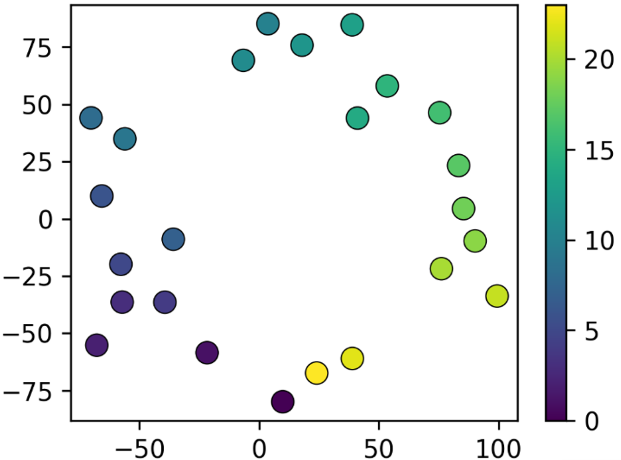
To better interpret the effectiveness of our model, we visualize the learned embeddings of absolute positional encoding. Due to the high dimension of the embeddings, t-SNE (Van der Maaten and Hinton 2008) is employed to visualize them on two-dimensional planes. The results are shown in Figure 6.
Figure 6 (a) shows that the embeddings of spatial encoding tend to cluster. Similar embeddings are either spatially proximate or exhibit analogous climatic patterns. Besides, the embeddings in Figure 6 (b) and (d) form ring-like structures in temporal order, revealing the distinct daily and annually periodicities of weather, which is consistent with our common understanding.


Conclusion
This work innovatively highlights the importance of absolute positional encoding in Transformer-based weather forecasting models. Even in the absence of attention mechanisms, absolute positional encoding can explicitly capture spatial-temporal correlations by integrating geographical coordinates and real-world time features, which are closely related to the evolution of atmospheric states in global weather system. Subsequently, we present LightWeather, a lightweight and effective weather forecasting model. We utilize the absolute positional encoding and replace the main components of Transformer with an MLP. Extensive experiments demonstrate that LightWeather can achieve satisfactory performance on global weather datasets, and the simple structure endows it with high efficiency and scalability to fine-grained data. This work posits that the incorporation of geographical and temporal knowledge is more effective than relying on intricate model architectures. This approach is anticipated to have a substantial impact beyond the realm of weather forecasting, extending its relevance to the predictions that involve geographical information (e,g., air quality and marine hydrology) and illuminating a new direction for DL approaches in these domains. In future work, we plan to integrate the model with physical principles more closely to enhance its interpretability.
References
- Bauer, Thorpe, and Brunet (2015) Bauer, P.; Thorpe, A.; and Brunet, G. 2015. The quiet revolution of numerical weather prediction. Nature, 525(7567): 47–55.
- Bernardes et al. (2023) Bernardes, G. F.; Ishibashi, R.; Ivo, A. A.; Rosset, V.; and Kimura, B. Y. 2023. Prototyping low-cost automatic weather stations for natural disaster monitoring. Digital Communications and Networks, 9(4): 941–956.
- Bi et al. (2023) Bi, K.; Xie, L.; Zhang, H.; Chen, X.; Gu, X.; and Tian, Q. 2023. Accurate medium-range global weather forecasting with 3D neural networks. Nature, 619(7970): 533–538.
- Bian et al. (2021) Bian, Y.; Huang, J.; Cai, X.; Yuan, J.; and Church, K. 2021. On attention redundancy: A comprehensive study. In Proceedings of the 2021 conference of the north american chapter of the association for computational linguistics: human language technologies, 930–945.
- Chen et al. (2023) Chen, L.; Du, F.; Hu, Y.; Wang, Z.; and Wang, F. 2023. Swinrdm: integrate swinrnn with diffusion model towards high-resolution and high-quality weather forecasting. In Proceedings of the AAAI Conference on Artificial Intelligence, volume 37, 322–330.
- Cui, Xie, and Zheng (2021) Cui, Y.; Xie, J.; and Zheng, K. 2021. Historical inertia: A neglected but powerful baseline for long sequence time-series forecasting. In Proceedings of the 30th ACM international conference on information & knowledge management, 2965–2969.
- Deng et al. (2024) Deng, J.; Song, X.; Tsang, I. W.; and Xiong, H. 2024. Parsimony or Capability? Decomposition Delivers Both in Long-term Time Series Forecasting. arXiv preprint arXiv:2401.11929.
- Huang et al. (2024) Huang, S.; Liu, Y.; Cui, H.; Zhang, F.; Li, J.; Zhang, X.; Zhang, M.; and Zhang, C. 2024. MEAformer: An all-MLP transformer with temporal external attention for long-term time series forecasting. Information Sciences, 669: 120605.
- Jin et al. (2024) Jin, M.; Wang, S.; Ma, L.; Chu, Z.; Zhang, J. Y.; Shi, X.; Chen, P.-Y.; Liang, Y.; Li, Y.-F.; Pan, S.; et al. 2024. Time-LLM: Time Series Forecasting by Reprogramming Large Language Models. In The Twelfth International Conference on Learning Representations.
- Kingma and Ba (2014) Kingma, D. P.; and Ba, J. 2014. Adam: A method for stochastic optimization. arXiv preprint arXiv:1412.6980.
- Lam et al. (2023) Lam, R.; Sanchez-Gonzalez, A.; Willson, M.; Wirnsberger, P.; Fortunato, M.; Alet, F.; Ravuri, S.; Ewalds, T.; Eaton-Rosen, Z.; Hu, W.; et al. 2023. Learning skillful medium-range global weather forecasting. Science, 382(6677): 1416–1421.
- Li et al. (2023) Li, Z.; Rao, Z.; Pan, L.; and Xu, Z. 2023. Mts-mixers: Multivariate time series forecasting via factorized temporal and channel mixing. arXiv preprint arXiv:2302.04501.
- Liang et al. (2023) Liang, Y.; Xia, Y.; Ke, S.; Wang, Y.; Wen, Q.; Zhang, J.; Zheng, Y.; and Zimmermann, R. 2023. Airformer: Predicting nationwide air quality in china with transformers. In Proceedings of the AAAI Conference on Artificial Intelligence, volume 37, 14329–14337.
- Lin et al. (2022) Lin, H.; Gao, Z.; Xu, Y.; Wu, L.; Li, L.; and Li, S. Z. 2022. Conditional local convolution for spatio-temporal meteorological forecasting. In Proceedings of the AAAI conference on artificial intelligence, volume 36, 7470–7478.
- Lin et al. (2024) Lin, S.; Lyu, P.; Liu, D.; Tang, T.; Liang, X.; Song, A.; and Chang, X. 2024. MLP Can Be A Good Transformer Learner. In Proceedings of the IEEE/CVF Conference on Computer Vision and Pattern Recognition, 19489–19498.
- Marchuk (2012) Marchuk, G. 2012. Numerical methods in weather prediction. Elsevier.
- Ni, Wang, and Fang (2022) Ni, Q.; Wang, Y.; and Fang, Y. 2022. GE-STDGN: a novel spatio-temporal weather prediction model based on graph evolution. Applied Intelligence, 52(7): 7638–7652.
- Nie et al. (2023) Nie, Y.; Nguyen, N. H.; Sinthong, P.; and Kalagnanam, J. 2023. A Time Series is Worth 64 Words: Long-term Forecasting with Transformers. In The Eleventh International Conference on Learning Representations.
- Schultz et al. (2021) Schultz, M. G.; Betancourt, C.; Gong, B.; Kleinert, F.; Langguth, M.; Leufen, L. H.; Mozaffari, A.; and Stadtler, S. 2021. Can deep learning beat numerical weather prediction? Philosophical Transactions of the Royal Society A, 379(2194): 20200097.
- Shao et al. (2023) Shao, Z.; Wang, F.; Xu, Y.; Wei, W.; Yu, C.; Zhang, Z.; Yao, D.; Jin, G.; Cao, X.; Cong, G.; et al. 2023. Exploring progress in multivariate time series forecasting: Comprehensive benchmarking and heterogeneity analysis. arXiv preprint arXiv:2310.06119.
- Shao et al. (2022) Shao, Z.; Zhang, Z.; Wang, F.; Wei, W.; and Xu, Y. 2022. Spatial-temporal identity: A simple yet effective baseline for multivariate time series forecasting. In Proceedings of the 31st ACM International Conference on Information & Knowledge Management, 4454–4458.
- Shumway, Stoffer, and Stoffer (2000) Shumway, R. H.; Stoffer, D. S.; and Stoffer, D. S. 2000. Time series analysis and its applications, volume 3. Springer.
- Sose and Sayyad (2016) Sose, D. V.; and Sayyad, A. D. 2016. Weather monitoring station: a review. Int. Journal of Engineering Research and Application, 6(6): 55–60.
- Tenzin et al. (2017) Tenzin, S.; Siyang, S.; Pobkrut, T.; and Kerdcharoen, T. 2017. Low cost weather station for climate-smart agriculture. In 2017 9th international conference on knowledge and smart technology (KST), 172–177. IEEE.
- Van der Maaten and Hinton (2008) Van der Maaten, L.; and Hinton, G. 2008. Visualizing data using t-SNE. Journal of machine learning research, 9(11).
- Vaswani et al. (2017) Vaswani, A.; Shazeer, N.; Parmar, N.; Uszkoreit, J.; Jones, L.; Gomez, A. N.; Kaiser, Ł.; and Polosukhin, I. 2017. Attention is all you need. Advances in neural information processing systems, 30.
- Wang et al. (2019) Wang, B.; Lu, J.; Yan, Z.; Luo, H.; Li, T.; Zheng, Y.; and Zhang, G. 2019. Deep uncertainty quantification: A machine learning approach for weather forecasting. In Proceedings of the 25th ACM SIGKDD international conference on knowledge discovery & data mining, 2087–2095.
- Wu et al. (2023a) Wu, H.; Hu, T.; Liu, Y.; Zhou, H.; Wang, J.; and Long, M. 2023a. TimesNet: Temporal 2D-Variation Modeling for General Time Series Analysis. In The Eleventh International Conference on Learning Representations.
- Wu et al. (2023b) Wu, H.; Zhou, H.; Long, M.; and Wang, J. 2023b. Interpretable weather forecasting for worldwide stations with a unified deep model. Nature Machine Intelligence, 5(6): 602–611.
- Wu et al. (2019) Wu, Z.; Pan, S.; Long, G.; Jiang, J.; and Zhang, C. 2019. Graph wavenet for deep spatial-temporal graph modeling. arXiv preprint arXiv:1906.00121.
- Yu et al. (2023) Yu, C.; Wang, F.; Shao, Z.; Sun, T.; Wu, L.; and Xu, Y. 2023. Dsformer: A double sampling transformer for multivariate time series long-term prediction. In Proceedings of the 32nd ACM international conference on information and knowledge management, 3062–3072.
- Yu et al. (2024a) Yu, C.; Wang, F.; Wang, Y.; Shao, Z.; Sun, T.; Yao, D.; and Xu, Y. 2024a. MGSFformer: A Multi-Granularity Spatiotemporal Fusion Transformer for Air Quality Prediction. Information Fusion, 102607.
- Yu et al. (2024b) Yu, C.; Yan, G.; Yu, C.; Liu, X.; and Mi, X. 2024b. MRIformer: A multi-resolution interactive transformer for wind speed multi-step prediction. Information Sciences, 661: 120150.
- Yu et al. (2022) Yu, W.; Luo, M.; Zhou, P.; Si, C.; Zhou, Y.; Wang, X.; Feng, J.; and Yan, S. 2022. Metaformer is actually what you need for vision. In Proceedings of the IEEE/CVF conference on computer vision and pattern recognition, 10819–10829.
- Zeng et al. (2023) Zeng, A.; Chen, M.; Zhang, L.; and Xu, Q. 2023. Are transformers effective for time series forecasting? In Proceedings of the AAAI conference on artificial intelligence, volume 37, 11121–11128.
- Zhou et al. (2021) Zhou, H.; Zhang, S.; Peng, J.; Zhang, S.; Li, J.; Xiong, H.; and Zhang, W. 2021. Informer: Beyond efficient transformer for long sequence time-series forecasting. In Proceedings of the AAAI conference on artificial intelligence, volume 35, 11106–11115.
- Zhou et al. (2022) Zhou, T.; Ma, Z.; Wen, Q.; Wang, X.; Sun, L.; and Jin, R. 2022. Fedformer: Frequency enhanced decomposed transformer for long-term series forecasting. In International conference on machine learning, 27268–27286. PMLR.
- Zhou et al. (2023) Zhou, T.; Niu, P.; Sun, L.; Jin, R.; et al. 2023. One fits all: Power general time series analysis by pretrained lm. Advances in neural information processing systems, 36: 43322–43355.
Appendix A Thereotical Proofs
A.1 Proof of Corollary 1.1
Proof.
According to Theorem 1 , we have
| (12) |
where is the interval between time steps.
For brevity, is denoted as . We can split into two parts, then we have
| (13) |
By repeating this procedure for the subsequent values of , we have
| (14) |
Let and denotes , then Eq. (14) can be expressed as
| (15) |
The weighted sum of is a function of , thus we have
| (16) |
∎
A.2 Proof of Theorem 2
Proof.
The data embedding layer maps the input data into latent space with dimension , thereby introducing parameters. Analogously, the regression layer introduces parameters. For the positional encoding, spatial encoding costs parameters, and temporal encoding costs parameters. The parameter count of a -layer MLP with residual connect is . Thus, the total number of parameters is The total number of parameters required for the LightWeather is . ∎
Appendix B Experimental Details
B.1 Datasets Description
In order to evaluate the comprehensive performance of the proposed model, we conduct experiments on 5 weather datasets with different temporal resolutions and spatial coverages including:
-
•
GlobalWind and GlobalTemp are collected from the National Centers for Environmental Information (NCEI)111https://www.ncei.noaa.gov/data/global-hourly/access. These datasets contains the hourly averaged wind speed and temperature of 3,850 stations around the world, spanning two years from 1 January 2019 to 31 December 2020. Kindly note that these datasets are rescaled (multiplied by ten times) from the raw datasets.
-
•
Wind_CN and Temp_CN are also collected from NCEI222https://www.ncei.noaa.gov/data/global-summary-of-the-day/access. These datasets contains the daily averaged wind speed and temperature of 396 stations in China (382 stations for Temp_CN due to missing values), spanning 10 years from 1 January 2013 to 31 December 2022.
-
•
Wind_US is collected from Kaggle333https://www.kaggle.com/datasets/selfishgene/historical-hourly-weather-data. It contains the hourly averaged wind speed of 27 stations in US, spanning 62 months from 1 October 2012 to 30 November 2017. The original dataset only provide the latitudes and longitudes of stations and we obtain the elevations of stations through Google Earth444https://earth.google.com/web.
The statistics of datasets are shown in Table 5, and the distributions of stations are shown in Figure 7.
| Dataset | Coverage | Station | Sample | Time | Length |
|---|---|---|---|---|---|
| Num | Rate | Span | |||
| GlobalWind | Global | 3850 | 1 hour | 2 years | 17,544 |
| GlobalTemp | Global | 3850 | 1 hour | 2 years | 17,544 |
| Wind_CN | National | 396 | 1 day | 10 years | 3,652 |
| Temp_CN | National | 382 | 1 day | 10 years | 3,652 |
| Wind_US | National | 27 | 1 hour | 62 months | 45,252 |


B.2 Introduction to the Baselines
-
•
HI (Cui, Xie, and Zheng 2021), short for historical inertia, is a simple baseline that adopt most recent historical data as the prediction results.
-
•
ARIMA (Shumway, Stoffer, and Stoffer 2000) , short for auto regressive integrated moving average, is a statistical forecasting method that uses the combination of historical values to predict the future values.
-
•
Informer (Zhou et al. 2021) is a Transformer with a sparse self-attention mechanism.
-
•
FEDformer (Zhou et al. 2022) is a frequency enhanced Transformer combined with seasonal-trend decomposition to capture the overall trend of time series.
-
•
DSformer (Yu et al. 2023) utilizes double sampling blocks to model both local and global information.
-
•
PatchTST (Nie et al. 2023) divides the input time series into patches, which serve as input tokens of Transformer.
-
•
TimesNet (Wu et al. 2023a) transforms time series into 2D tensors and utilizes a task-general backbone that can adaptively discover multi-periodicity and extract complex temporal variations from transformed 2D tensors.
-
•
GPT4TS (Zhou et al. 2023) employs pretrained GPT2 backbone and a linear layer to obtain the output.
-
•
Time-LLM (Jin et al. 2024) reprograms the input time series with text prototypes before feeding it into the frozen LLM backbone to align time series with natural language modality.
-
•
DLinear (Zeng et al. 2023) is a linear model with time series decomposition.
-
•
AirFormer (Liang et al. 2023) employs a dartboard-like mapping and local windows to restrict attentions to focusing solely on local information.
-
•
Corrformer (Wu et al. 2023b) utilizes a decomposition framework and replaces attention mechanisms with a more efficient multi-correlation mechanism.
-
•
MRIformer (Yu et al. 2024b) employs a hierarchical tree structure, stacking attention layers to capture correlations from multi-resolution data obtained by down sampling.
| Dataset | GlobalWind | GlobalTemp | ||
|---|---|---|---|---|
| Metric | MSE | MAE | MSE | MAE |
| ERA5 (0.5°) | 6.793 | 1.847 | 28.07 | 3.270 |
| GFS (0.25°) | 9.993 | 2.340 | 14.93 | 2.287 |
| LightWeather | 3.734 | 1.295 | 7.420 | 1.858 |
B.3 Comparison with Numerical Methods
In this section, we compare our model to numerical weather prediction (NWP) methods. Conventional NWP methods uses partial differential equations (PDEs) to describe the atmospheric state transitions across grid points and solve them through numerical simulations. Currently, the ERA5 from European Centre for Medium-Range Weather Forecasts (ECMWF) and the Global Forecast System (GFS) from NOAA are the most advanced global forecasting models. ERA5 provides gridded global forecasts at a 0.5° resolution while GFS at a 0.25° resolution.
To make the comparison pratical, we utilize bilinear interpolation with height correction to obtain the results for scattered stations, which is aligned with the convention in weather forecasting (Bauer, Thorpe, and Brunet 2015). The results are shown in Table 6.
Both ERA5 and GFS fail to provide accurate preictions, which indicates that grid-based NWP methods are inadequate for fine-grained station-based predictions. Conversely, LightWeather can accurately forecast the global weather for worldwide stations, significantly outperforming the numerical methods.
Appendix C Overall Workflow
The overall workflow of LightWeather is shown in Algorithm 1.