Light-induced swirling and locomotion
Abstract
Photomechanical liquid crystal elastomers (LCEs) are responsive polymers that can convert light directly into mechanical deformation. This unique feature makes these materials an attractive candidate for soft actuators capable of remote and multi-mode actuation. In this work, we propose a three-dimensional multi-scale model of the nonlinear and nonlocal dynamics of fibers of photomechanical LCEs under illumination. We use the model to show that a pre-stressed helix-like fibers immersed in a fluid can undergo a periodic whirling motion under steady illumination. We analyze the photo-driven spatiotemporal pattern and stability of the whirling deformation, and provide a parametric study. Unlike previous work on photo-driven periodic motion, this whirling motion does not exploit instabilities in the form of snap-through phenomena, or gravity as in rolling. We then show that such motion can be exploited in developing remote controlled bio-inspired microswimmers and novel micromixers.
Keywords
Photomechanical materials; Liquid crystal elastomers; Whirling actuation; Propulsion.
Significance
The design of untethered devices with no or limited onboard power that can be activated remotely remains a continuing challenge in soft robotics. This work addresses this challenge by developing a method of generating a whirling motion in a pre-stressed photomechanical liquid crystal elastomer fiber using steady illumination, and then showing how this motion may be exploited for applications such as microswimmers and micromixers. More broadly, this provides an unusual example of a physical system capable of periodic motion under steady stimulus that does not exploit instabilities.
1 Introduction
Liquid crystal elastomers (LCEs) are rubbery networks composed crosslinked polymer chains that contain liquid-crystalline mesogens in their main or in side chains. External stimuli like heat changes the ordering of the liquid-crystalline (LC) mesogens leading to a change in shape or stimuli-induced deformation. This phenomenon is reversible. LCEs containing light-sensitive molecules, such as azobenzene (azo) photochromes, exhibit a reversible photomechanical behavior: they absorb light energy and convert it into mechanical energy by changing their shape. This fascinating photomechanical effect arises from the trans-cis isomerization of azobenzene dyes, a process in which the azo molecules absorb light energy and change their conformation from a linear trans isomer to a bent cis isomer. The steric interaction between the azo and LC molecules consequently changes the LC ordering leading to a photo-induced shape-change. Upon removing the light, the cis isomers thermally relax to the trans state leading to a reversal of the photo-induced shape-change.
Recent works demonstrate the potential of photomechanical materials for soft robotics because of their remarkable features: 1) properly synthesized photomechanical materials can undergo large, reversible deformation upon light irradiation, 2) these materials are lightweight and soft, and hence, appropriate to generate flexible motion in soft robotics, 3) light is a clean power source that can actuate a photomechanical object from distance, thereby eliminating the need for on-board power or tethers, and 4) light-induced deformations can be controlled by changing light intensity, wavelength, or polarization [1, 2, 3] thereby providing a platform for multiplexing and control.
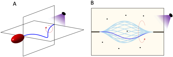
In particular, recent attention has focussed on locomotion in soft-robotics. A long-standing problem in the use of active materials is the need to reset the material after each actuation stroke. The ability to rapidly turn on and turn off light enables such a reset. This has been exploited to build legged microwalkers [4], leg-free caterpillar-like crawling [5] and swimming flagellum [6]. Even more promising, the coupling between photo-isomerization, light propagation and nonlinear mechanics can be exploited to generate cyclic motion even under steady illumination. Yamada et al. [7] demonstrated a ring can be made to roll by simultaneously illuminating it with a combination of UV and natural light at two different but carefully chosen locations. Wie et al. [8] demonstrated that a flat monolithic polymer films made of azo-containing liquid crystalline polymer networks changes its conformation to a spiral ribbon under illumination. The ribbon also translates a large distance with continuous irradiation. Gelebart et al. [9] created a wave like motion a doubly clamped azo-LCE strip using steady illumination and exploited this for a framed walker under steady illumination. In these examples, the motion is generated by gravity and the reaction from the surface. In this work, we explore cyclic motion under steady illumination in an immersive environment, and propose potential applications as bio-inspired micro-swimmers and micro-mixers as shown in Figure 1.
The generation of cyclic deformation has also been a subject of interest in chemo-mechanical systems since the demonstration of oscillatory swelling and deswelling in hydrogels [10, 11]. In these systems, cyclic chemistry like the Belousov-Zhabotinsky reactions or Landolt pH oscillators are combined with hydrogels to obtain a chemo-mechanical oscillations. These have recently been used to demonstrate spatio-temporal oscillatory motion that can be exploited for peristaltic motion and walking [12], as well as homeostatic feedback loops [13]. A theoretical model of these systems show that the system is statically bistable and the dissipative kinetics leads to a these chemo-mechanical oscillations. In this way, these systems are conceptually similar to the wave like motion [9]. In this work, we explore the emergence of periodic behavior in a stable system.
We begin by developing a three-dimensional theory of photomechanical rods. The general theory of photomechanical coupling was developed by Corbett and Warner [14], and used by Warner and Mahadevan [15] to study the development of light-induced spontaneous curvature in beams and plates under the assumption of shallow penetration. Corbett et al. [16] studied deep penetration, and the deformation of beams under stress-free conditions (i.e., without loads). Korner et al. [17] developed the theory of photomechanical beams under loads and used it to explain the rolling of rings [7] and wave-like motion of doubly-clamped beams [9]. All of this work was limited to the two-dimensional setting of beams. In this paper, we extend these ideas to the three dimensional setting of rods by combining the photomechanical actuation with nonlinear Kirchhoff rod theory. We do so in a dynamical setting with inertia.
We then use the theory to exploit photomechanical coupling and pre-stressed structural configuration to generate periodic whirling motion under steady illumination; a fascinating photomechanical response that, to our knowledge, has not been reported in literature. Importantly, we show that such whirling motion of a fiber immersed in a viscous fluid generates propulsion along its rotational axis. This can be exploited in developing remote controlled bio-inspired microswimmers and micromixers (Figure 1). We also show that this phenomenon does not rely on instabilities of flapping, or on gravity. Finally, we show that we can control the photoresponse using illumination conditions (light intensity and direction), pre-stressed configuration of fiber (twist and bending) and cross-sectional shape (circular and rectangular). These provide opportunities to design microactuators for different conditions, and for control. Together, the model and the results open a new avenue for the development of remote actuated and controlled soft actuators.
2 Model
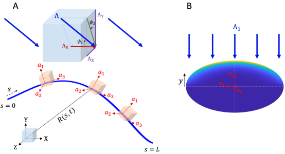
Consider a long, thin azo-LCE fiber subjected to a steady illumination that makes angles and with fixed frame XYZ as illustrated in Figure 2A. We describe the centerline of fiber as a time-dependent space curve where is the arc-length along the fiber and is time. Let be a body-fixed orthonomal frame at point and time with unit vectors and coinciding with the principal axes of the cross-section and normal to the cross-section. We assume that the fiber is inextensible and unshearable so that is always tangent to the space curve. We define the curvature vector in the frame. Note that the rod may have intrinsic (stress-free, illumination free) curvature.
We now specify the photomechanical constitutive behavior of the rod building on the ideas of [14, 17]. Consider a short section of the filament at position and time . Suppose for the moment that it is subjected to an illumination along axis with intensity as shown in Figure 2B. As the light diffracts into the cross-section, it is absorbed by the photochrome molecules and attenuates. In this work, we assume shallow penetration governed by Beer’s law. Recall that, according to Beer’s law, when a light impinges on a flat surface with intensity , the intensity at a depth is given by where is the penetration depth. Generalizing this to our general cross-section, the intensity at any point on the cross-section is given by for some function which quickly decays to zero away from the surface as illustrated in Figure 2B. Examples of this function are provided in the supplementary material.
The photochromes in the trans state absorb light and transform into the cis state which can thermally relax back to the trans state. Therefore, the number density of cis molecules at position evolves according to
| (1) |
where the dot represents the material time derivative, is thermal relaxation time (or lifetime), and is a constant depending on material properties and forward-backward reaction rates. This in turn introduces a spontaneous axial strain where is a constant of proportionality with corresponds to a contraction. It follows that the axial normal stress where , is the intrinsic (stress-free, illumination-free) curvature in the 2-direction, and is the Young’s modulus. The bending moment along the is
| (2) |
where is the bending rigidity along and is the second moment of inertia along . Now, differentiating with respect to time and using (1), we conclude that
| (3) |
In the case of general illumination, we split it into components along and to conclude that the photomechanical constitutive behavior of the beam is given by
| (4) | |||
| (5) |
where is the vector of bending moments and torque, is the tensorial rigidity (diag in the basis with bending and torsional rigidities and is the photomechanical rate tensor (diag in the basis).
Finally, we complete the system of equations by considering the balance of linear and angular momenta [18, 19],
| (6) | |||
| (7) |
where is the particle velocity, is the spatial time derivative, the angular velocity of the frame , and and are the external or applied force and moment per unit length respectively; the inextensibility
| (8) |
the compatibility between curvature and angular velocity
| (9) |
and appropriate initial and boundary conditions.
If the fiber is immersed in a fluid, it experiences a hydrodynamic drag force per unit length that acts as the external force in (6):
| (10) |
where the normal, bi-normal, and tangential drag coefficients are estimated to be and for a circular cross-section, respectively, in the limit of low Reynolds number [20]. Above, is the dynamic viscosity of fluid, and and are the length and diameter of fiber, respectively. The drag force is incorporated into the dynamic model through the term in (6).
To solve the nonlinear initial-boundary-value problem above, we employ a finite difference method in both space and time to discretize the equations. Starting with the initial condition of fiber at , the discretized equations are integrated over space at each successive time step. During spatial integration, the boundary conditions are satisfied using the shooting method for boundary-value problems. For details on the numerical method, see [21, 22, 23].
3 Photo-driven motion of a buckled and twisted fiber
We now use the model to study the deformation of initially straight () fibers with circular ( ) cross-section that are buckled and possibly twisted, clamped at the two ends and illuminated. We use the parameters listed in Table 1 unless otherwise specified. A detailed parameter study is provided in supplementary information.
| Parameter (symbol) | Value |
|---|---|
| Young’s modulus () | 4 GPa [24] |
| Fiber diameter () | 15 m [24] |
| Fiber length () | 15 mm [24] |
| Penetration depth () | 0.56 m [17] |
| Relaxation time () | 0.1 s |
| cis-strain proportionality () | 0.05 |
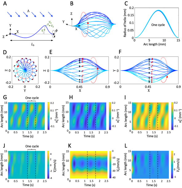
We begin by defining a pre-stressed doubly clamped conformation as the initial state of the fiber. Assume that the fiber is initially straight () with length and the nematic director is along the axis of the fiber (so in Eq. (2)). We compress and twist the fiber quasi-statically by applying a compressive force along and a torque about the axis of fiber till the fiber buckles (the final end to end distance is and angle of twist is ). We then clamp the two ends by constraining their position and rotation till the fiber is in equilibrium. This is initial state of fiber which we then illuminate as shown in Figure 3A.
Typical result
A typical result () is shown in Figure 3B-L. After an initial transient, the fiber undergoes a steady cyclic motion, snapshots of which over one cycle are displayed in Figure 3B (in perspective view) and D-F (three normal projections). Note from Figure 3D that the rotation about the X axis (line joining the end points) is uniform and from Figure 3E,F that the shape is slightly asymmetric about the X-axis and about the center. Snapshots of the radial distance (distance to the line joining the end points) during the cycle is shown in Figure 3C; note that this is almost invariant. In short, the buckled and twisted fiber rotates about the axis quite uniformly and with an almost a rigid shape. However, the rotation is not rigid since the ends are clamped. Figure 3G-I plot the spatio-temporal evolution of the spontaneous curvature of the fiber (components of with respect to the laboratory frame) over first five cycles, while Figure 3J-L plot the velocity. These confirm that the motion is indeed periodic after an initial transient. We also note that after an initial transient, the radial and axial components of velocity remain very small confirming the almost fixed shape we observed earlier. The angular velocity shows small periodic fluctuations showing that the rotational motion is almost, but perfectly, uniform.
As the fiber is illuminated, the photomechanical coupling causes a change in spontaneous curvature which leads to a change of shape. The overall length of the fiber endows it with a very small twisting stiffness, and this enables the fiber to accommodate this change of shape by a rotary motion. This changes the illumination conditions (the angle between the direction of light propagation and the tangent to the fiber) leading to a further change of shape and this cascades into a cyclic motion that we observe. We emphasize that the fiber is clamped at both ends, so it is not free to rotate about the X-axis. This is consistent with the periodic fluctuations in the angular velocity. Still, the small twisting stiffness makes this a low energy manifold of deformation, thereby enabling the motion. Importantly, there is no instability which we discuss further in the case with zero twist.
Zero twist
We now consider the case of zero twist (). The pre-stressed shape is planar and we assume that it belongs to the XY plane as shown schematically in Figure 4A. There are two cases. The first is the planar case where the illumination is also in the XY plane (). This is exactly the situation studied by Gelebart et al. [9] experimentally (though they used a strip) and through modeling by Korner et al. [17] (though they used a quasistatic model with no inertia). When illuminated, we observe that the fiber goes into a flapping motion as shown in Figure 4B coinciding with the results of Korner et al. [17]. The second case is the non-planar case where the illumination is not in the XY plane (). In this case, we see in Figure 4C that the fiber goes into whirling motion similar to that of the case with twist.
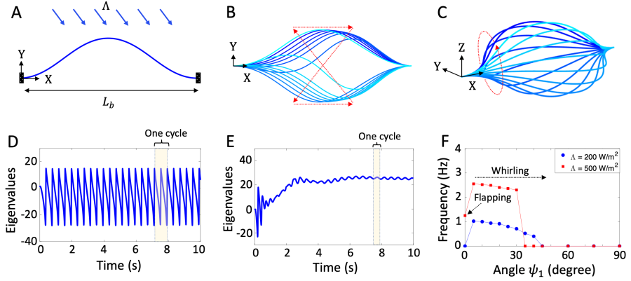
There is a crucial difference between the flapping motion in the planar case and the whirling motion in the non-planar case. Korner et al. [17] showed that the flapping motion in the planar case is enabled by snap-through buckling instability between two distinct buckled states. This is also shown in Figure 4B where the arrows trace the position of the peak during one cycle. There are two segments where the evolution is slow as the peak/trough moves to the right (dashed horizontal arrows), and two segments where the evolution is fast as the fiber snaps between the up and down buckled states (diagonal arrows). The snap-through is confirmed by analyzing the stability by examining the smallest eigenvalue of the stiffness matrix in Figure 4D. We note that this becomes negative indicating instability. In contrast, the motion in whirling is always smooth and there is no instability. This is confirmed by analyzing the stability by examining the smallest eigenvalue of the stiffness matrix in Figure 4E. This is also in the case of an initially buckled and twisted fiber () (see supplemental information). Figure 4F shows he frequency of flapping is smallter than that of whirling.
4 Photo-driven propulsion
We now examine whether the photo-driven motion discussed in the previous section can be used to generate propulsion. We consider that the fiber is immersed in a fluid and therefore subject to a hydrodynamic drag force. The total drag force on the filament in laboratory frame is given by integrating the drag force per unit length over the length of the filament
| (11) |
Further, the average propulsive force over the cycle is
| (12) |
where is the period.
We assume that the fiber is attached to a bead, and therefore this force propels the bead through the fluid with the velocity where is the drag coefficient for the bead and is the velocity of bead in laboratory frame. We solve the equations of the fiber to obtain the total force, and then use this force to study the motion of the bead. We now describe results where the immersing fluid is water with viscosity of Pa.s, and for simplicity, we assume is identity.
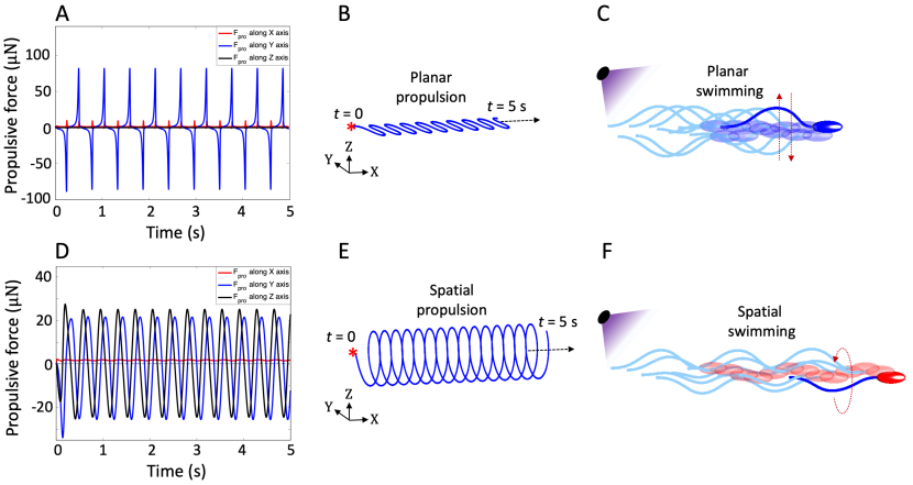
Figure 5 shows the results for a planar fiber () with a flapping motion and a spatial fiber () with a whirling motion. We first consider the planar case. Figure 5A shows that the propulsive force is periodic after an initial transient; this is expected since the motion and the velocity of fiber are periodic as noted earlier. There is a large propulsive force in the that is normal to the axis of the fiber; however the average of this force is zero. The propulsive force in the Z direction normal to the plane is zero as expected. Finally, we have spikes in the propulsive force in the X direction during the snap-through phase of the cycle; importantly, this is always in the same direction, and thus the net propulsive force (Eq. (12)) in the X direction is non-zero. All of this leads to the motion of the bead shown in Figure 5B. Note that it follows a sinusoidal path of cyclic excursions in the Y direction that produce no net translation, but a quasi-steady motion in the X direction. This sinusoidal trail is reminiscent of the crawling of the nematode and C. elegance.
We then turn to the spatial case. Figure 5C shows that the propulsive force is periodic after an initial transient as expected. Once again we see large forces in the Y and Z directions, but they average to zero. However, there is a small but steady force in the X direction. This leads to the helical or spiral motion as shown in Figure 5D that is reminiscent of swimming of sperm and flagellated bacteria.
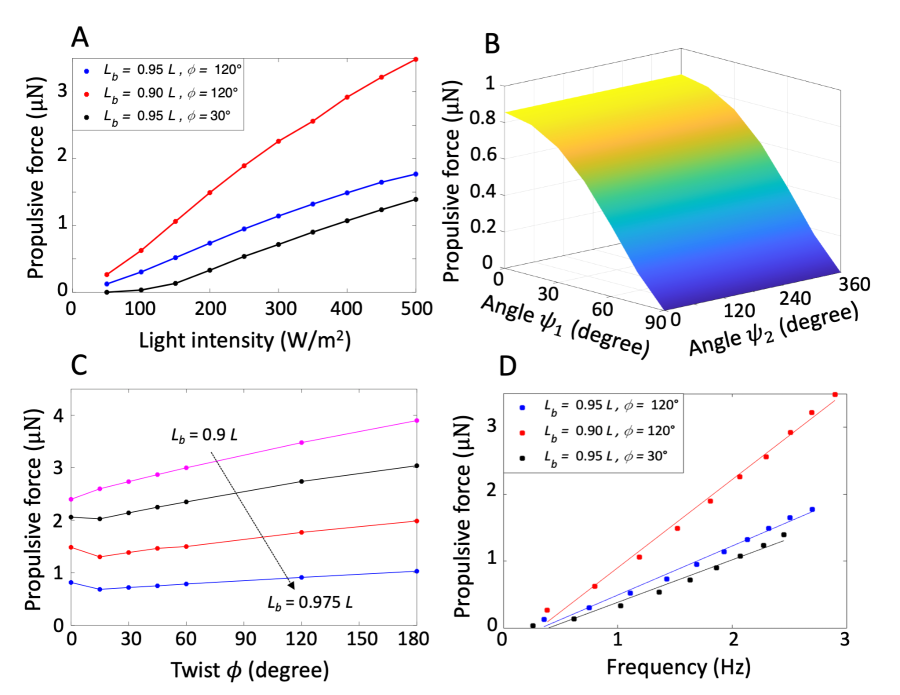
Figure 6 presents a parameter study. Figure 6A shows that the average propulsive force over the cycle increases with illumination. This is consistent with our finding that the frequency increases with illumination (cf. supplementary information). Figure 6B shows that the role of illumination direction, and this reflects the dependance of the frequency since the twist and the buckled length remain the same. Similarly, Figure 6C shows that propulsive force increases with increasing twist, and that this increase is greater than that can be expected from the increase of frequency alone (cf. supplementary information). Also, the propulsive force increases with decreasing , and that this dependance is greater than that of the frequency.
Figure 6D shows that the propulsive force and the frequency are proportionally correlated. This is consistent with the resistive force theory and experimental data [25, 26] for a rotating rigid cylindrical helix at low Reynolds number that the propulsive thrust increases linearly with respect to rotation frequency. We note that the slight deviation from a perfect linear function can correspond to the slight deformation of fiber during rotation while its overall shape remains almost constant (cf. Figure 3).
Acknoweledgment
We gratefully acknowledge the support of the US Office of Naval Research through Multi-investigator University Research Initiative Grant ONR N00014-18-1-2624.
References
- [1] K. Kumar, C. Knie, D. Bléger, M.A. Peletier, H. Friedrich, S. Hecht, D.J. Broer, M.G. Debije, and A.P.H.J. Schenning. A chaotic self-oscillating sunlight-driven polymer actuator. Nature Communications, 7:11975, 2016.
- [2] H. Zeng, P. Wasylczyk, D.S. Wiersma, and A. Priimagi. Light robots: bridging the gap between microrobotics and photomechanics in soft materials. Advanced Materials, 30:1703554, 2018.
- [3] N. Tabiryan, S. Serak, X-M. Dai, and T. Bunning. Polymer film with optically controlled form and actuation. Optics Express, 13:7442–7448, 2005.
- [4] H. Zeng, P. Wasylczyk, C. Parmeggiani, D. Martella, M. Burresi, and D.S. Wiersma. Light-fueled microscopic walkers. Advanced Materials, 27:3883–3887, 2015.
- [5] H. Zeng, O.M. Wani, and A. Wasylczyk, P.and Priimagi. Light-driven, caterpillar-inspired miniature inching robot. Macromolecular Rapid Communications, 391:1700224, 2018.
- [6] C. Huang, J. Lv, X. Tian, Y/ Wang, Y. Yu, and J. Liu. Miniaturized swimming soft robot with complex movement actuated and controlled by remote light signals. Scientific Reports, 5:17414, 2015.
- [7] M. Yamada, M. Kondo, J. Mamiya, Y. Yu, M. Kinoshita, C.J. Barrett, and T. Ikeda. Photomobile polymer materials: towards light-driven plastic motors. Angewandte Chemie, 120:5064–5066, 2008.
- [8] J.J. Wie, M.R. Shankar, and T.J. White. Photomotility of polymers. Nature Communications, 7:13260, 2016.
- [9] A.H. Gelebart, D. Jan Mulder, M. Varga, A. Konya, G. Vantomme, E.W. Meijer, R.L.B. Selinger, and D.J. Broer. Making waves in a photoactive polymer film. Nature, 546:632–636, 2017.
- [10] R. Yoshida, T. Takahashi, T. Yamaguchi, and H. Ichijo. Self-oscillating gel. Journal of the American Chemical Society, 118:5134–5135, 1996.
- [11] C.J. Crook, A. Smith, R.A. Jones, and A.J. Ryan. Chemically induced oscillations in a ph-responsive hydrogel. Physical Chemistry and Chemical Physics, 4:1367–1369, 2002.
- [12] R. Kim, Y.S. an Tamate, A.M. Akimoto, and R. Yoshida. Recent developments in self-oscillating polymeric systems as smart materials: from polymers to bulk hydrogels. Materials Horizons, pages 38–54, 2017.
- [13] X. He, M. Aizenberg, O. Kuksenok, L.D. Zarzar, A. Shastri, A.C. Balazs, and J. Aizenberg. Synthetic homeostatic materials with chemo-mechano-chemical self-regulation. Nature, 487:214–218, 2012.
- [14] D. Corbett and M. Warner. Nonlinear Photoresponse of Disordered Elastomers. Physical Review Letters, 96:237802, 2006.
- [15] M. Warner and L. Mahadevan. Photoinduced deformations of beams, plates, and films. Physical Review Letters, 92:134302, 2004.
- [16] D. Corbett, C. Xuan, and M. Warner. Deep optical penetration dynamics in photobending. Physical Review E, 92:013206, 2015.
- [17] K. Korner, A.S. Kuenstler, R.C. Hayward, B. Audoly, and K. Bhattacharya. A nonlinear beam model of photomotile structures. Proceedings of the National Academy of Sciences, 117:9762–9770, 2020.
- [18] E.H. Dill. Kirchhoff’s theory of rods. Archive for History of Exact Sciences, 44:1–23, 1992.
- [19] S. Goyal, N.C. Perkins, and C.L. Lee. Nonlinear dynamics and loop formation in kirchhoff rods with implications to the mechanics of dna and cables. Journal of Computational Physics, 209:371–389, 2005.
- [20] J. Howard. Mechanics of motor proteins and the cytoskeleton: Sinauer assoc. Sunderland, MA, 2001.
- [21] C. Gatti-Bono and N.C. Perkins. Physical and numerical modelling of the dynamic behavior of a fly line. Journal of sound and vibration, 255:555–577, 2002.
- [22] A. Maghsoodi, A. Chatterjee, I. Andricioaei, and N.C. Perkins. A first model of the dynamics of the bacteriophage t4 injection machinery. Journal of Computational and Nonlinear Dynamics, 11::041026, 2016.
- [23] J.I. Gobat, M.A. Grosenbaugh, and M.S. Triantofyllou. Generalized-alpha time integration solutions for hanging chain dynamics. Technical report, Woods Hole Oceanographic Instituteion, 2002.
- [24] M.L. Smith, M.R. Shankar, R. Backman, V.P. Tondiglia, K.M. Lee, M.E. McConney, D.H. Wang, L-S. Tan, and T.J. White. Designing light responsive bistable arches for rapid, remotely triggered actuation. In Behavior and Mechanics of Multifunctional Materials and Composites 2014, volume 9058, pages 121–130. SPIE, 2014.
- [25] B. Rodenborn, C-H Chen, H.L Swinney, B. Liu, and H.P. Zhang. Propulsion of microorganisms by a helical flagellum. Proceedings of the National Academy of Sciences, 110:E338–E347, 2013.
- [26] X. Zhong, K.W. Moored, V. Pinedo, J. Garcia-Gonzalez, and A.J. Smits. The flow field and axial thrust generated by a rotating rigid helix at low reynolds numbers. Experimental Thermal and Fluid Science, 46:1–7, 2013.
Supplementary Material
Light-induced swirling and locomotion
Ameneh Maghsoodi and Kaushik Bhattacharya
1 Photomechanical model of Azo-LCE fibers
Consider a long, thin azo-LCE fiber possessing circular cross-section. Under illumination, Azobenzene molecules absorb photons and transform between linear to bent configurations due to light absorption and thermal decay. Suppose for the moment that the fiber is subjected to an illumination with intensity . As a simple case, assume that illumination is along axis Y as shown in Figure 1A. As the light diffracts into the cross-section, it is absorbed by the photochrome molecules and attenuates. In this work, we assume shallow penetration governed by Beer’s law. Recall that, according to Beer’s law, when a light impinges on the flat surface of a strip with thickness , the intensity decreases with depth such that the intensity at any point on the cross-section is given by
| (1) |
where is the penetration depth. Similarly, for a fiber with circular cross-section shown in Figure 1A
| (2) |
where function .
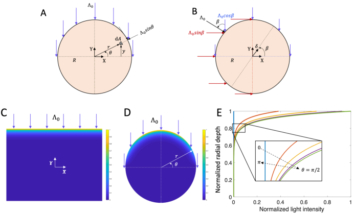
Figure 1C-E compares the light intensity profile for a circular and a rectangular cross-sections using (1) and (2). As shown in Figure 1C, the light intensity passing through a rectangular cross section decreases (exponentially) with depth . However, Figure 1D-E for a circular cross-section show that the light intensity depends on the depth as well as the angle between incident light and radial direction; where the maximum light intensity corresponds to and . Note that the light intensity at any angle decreases exponentially with radial depth (cf. (2)). This demonstrates that the fiber cross sectional shape affects the profile of light intensity.
The photochromes in the trans state absorb light and transform into the cis state which can thermally relax back to the trans state. Therefore, the number density of cis molecules along cross-section evolves according to
| (3) |
where the dot represents the material time derivative, is thermal relaxation time (or lifetime), and is a constant depending on material properties and forward-backward reaction rates. This in turn introduces a spontaneous axial strain where is a constant for proportionality with corresponds to a contraction. Consequently, the light-induced bending at the circular cross-section of the fiber
| (4) |
where
| (5) |
In (4), and denote the curvature and spontaneous stress-free curvature of the fiber, respectively. The constant is the bending stiffness with the second moments of area for a circular cross-section. Combining (3)-(5),
| (6) |
where
| (7) |
Now, in a general case, assume that a steady illumination makes angle with principal axis Y as illustrated in Figure 1B. Illumination makes bending about axis such that
| (8) |
| (9) |
On the other hand, illumination . Therefore, using (6)
| (10) |
| (11) |
Combining (6-11) concludes that photoactuaction by the steady illumination can be written as the sum of two photoactuactions and along principal axes X and Y, respectively.
2 Stability analysis
To examine stability of fiber for the dynamic equilibrium configurations, we calculate the second variation of total potential energy, . If , the potential energy is minimized at the equilibrium configuration, indicating that the configuration is stable. To derive the stability criteria, consider the potential energy function in the form
| (12) |
where and . To calculate the second variation of energy, we consider small variations around equilibrium configuration in the form
| (13) |
where is an arbitrary constant independent of and , and contains arbitrary functions which are independent of and satisfy boundary conditions. We differentiate twice with respect to and set to zero
| (14) |
From Rayleigh-Ritz approach, we assume , . In doing so, finding the minimum of second variation of energy subject to the constraint that becomes (by Lagrange multiplier ) an eigenvalue problem of finding . The positive eigenvalues imply that the configuration is stable. For a twisted-buckled rod that is clamped at one end and subjects to force and moment at the other end
| (15) |
Where , and in which is the rotation matrix from local frame to inertial frame.
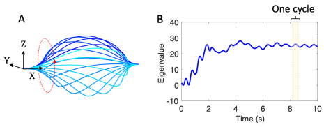
As shown in Figure 2A, a pre-stressed buckled-twisted fiber undergoes a periodic whirling motion under steady illumination. The motion in whirling is always smooth and there is no instability. This is confirmed by analyzing the stability by examining the smallest eigenvalue of the stiffness matrix in Figure 2B. The lowest eigenvalue is always positive.
3 Parameter Study
The effect of illumination intensity and direction
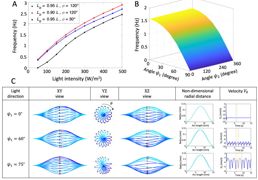
Figure 3 compares the frequency and pattern of oscillations over a range of values of illumination intensity and angles and . One needs a critical intensity before one has periodic motion (Figure 3A); below this critical intensity, the fiber deforms and attains a photo-stationary state. Beyond this critical intensity, the frequency increases with the light intensity: this is consistent with the fact that greater intensity leads to a higher rate of increase in the photo-induced strain and spontaneous curvature.
The angle between the direction of light propagation and the X-axis (the line joining the end-points) has a significant effect on the motion. When the illumination is perpendicular to the X-axis, then the fiber reaches a photo-stationary state (Figure 3B). The frequency increases as decreases and reaches a peak when the illumination is parallel to X-axis. There is symmetry about ; the illumination at angle drives fiber with the same velocity but opposite direction of illumination at angle .
Figure 3C shows that this angle also affects the shape of the rod, and the rotary motion becomes less steady as the illumination is perpendicular and the more steady as it is parallel to the X-axis. The angle which describes orientation in the YZ plane has no impact, consistent with almost rotary motion.
The effect of pre-stressed conformation of fiber
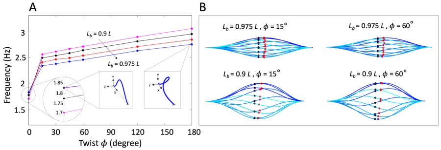
Figure 4 examines the frequency as a function of the pre-stressed conformation, both the buckled length and the angle of twist (with with and ). The figure shows that the case of no twist, , is distinct and so we defer its discussion. Once twisted, Figure 4A shows that the frequency increases almost linearly but only slightly with increasing twist. Increasing the buckling (i.e., reducing ) also increases the frequency. Figure 4B shows that the shape changes with a larger bulge with reduced .
Influence of illumination direction on the frequency and propulsion
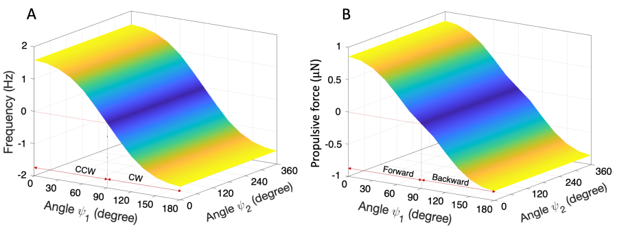
As shown in Figure 5, the whirling motion of a pre-stressed twisted-buckled fiber is symmetric with respect to the YZ plane perpendicular to the helical axis if fiber. Note that the amplitude of frequency and propulsive force are the same but the directions are the opposite with respect to YZ plane.
The effect of cross-sectional geometry
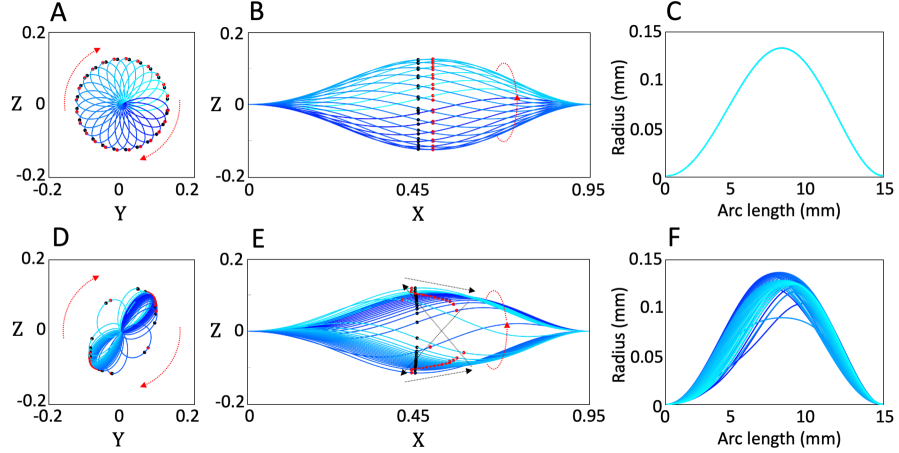
We now briefly examine whether the cross-section of fiber affects the photo-driven motion. In photomechanical model of fiber, the function depends on both geometrical and material properties of fiber. Examples of function are presented and compared for circular and rectangular cross section in the supplementary material. Figure 6 compares the photomechanical response of the fibers with square and rectangular cross sections where the illumination is along X-axis from left to right. From Figure 6A-C for a square cross-sectional fiber, the motion is periodic. The fiber rotates uniformly about its helical axis with an almost constant shape; this is similar to that of circular cross-sectional fiber explained in previous sections.
Figure 6D-F shows the photomechanical response of a rectangular cross-sectional fiber. The photo-driven motion is periodic; however, the pattern of deformation is significantly different from circular cross-sectional fiber. The fiber rotates about its axis, however, the rotation velocity is largely nonuniform during the cycle as observed in Figure 6D. From Figure 6E-F, the radial distance of fiber relative to rotation axis significantly changes. Also the maximum radius (Red dots) translates along X-direction while rotating about X-axis. These results concludes that the fiber undergoes a coupled flapping-whirling motion about its axis. Future analysis and parametric study on rectangular cross-section can reveal the contribution of bending and torsional elasticity and aspect ratio on the coupled flapping-whirling motion.
4 Animations
Planarpropulsion.mp4
Shows the motion of a bead attached to a buckled (but not twisted) fiber illuminated along the buckled plane.
Spatialpropulsion.mp4
Shows the motion of a bead attached to a buckled (but not twisted) fiber illuminated at an angle to the buckled plane.