LHS 1815b: The First Thick-Disk Planet Detected By TESS

Tianjun Gan Department of Astronomy and Tsinghua Centre for Astrophysics, Tsinghua University, Beijing 100084, China Avi Shporer Department of Physics and Kavli Institute for Astrophysics and Space Research, Massachusetts Institute of Technology, Cambridge, MA 02139, USA John H. Livingston Department of Astronomy, The University of Tokyo, 7-3-1 Hongo, Bunkyo-ku, Tokyo 113-0033, Japan Karen A. Collins Center for Astrophysics

{\rm\mid}

Harvard & Smithsonian, 60 Garden Street, Cambridge, MA 02138, USA Shude Mao Department of Astronomy and Tsinghua Centre for Astrophysics, Tsinghua University, Beijing 100084, China National Astronomical Observatories, Chinese Academy of Sciences, 20A Datun Road, Chaoyang District, Beijing 100012, China Alessandro A. Trani Department of Astronomy, The University of Tokyo, 7-3-1 Hongo, Bunkyo-ku, Tokyo 113-0033, Japan Davide Gandolfi Dipartimento di Fisica, Università degli Studi di Torino, via Pietro Giuria 1, I-10125, Torino, Italy Teruyuki Hirano Department of Earth and Planetary Sciences, Tokyo Institute of Technology, 2-12-1 Ookayama, Meguro-ku, Tokyo 152-8551, Japan Rafael Luque Instituto de Astrofísica de Canarias (IAC), 38205 La Laguna, Tenerife, Spain Departamento de Astrofísica, Universidad de La Laguna (ULL), 38206, La Laguna, Tenerife, Spain Keivan G. Stassun Department of Physics and Astronomy, Vanderbilt University, 6301 Stevenson Center Ln., Nashville, TN 37235, USA Department of Physics, Fisk University, 1000 17th Avenue North, Nashville, TN 37208, USA Carl Ziegler Dunlap Institute for Astronomy and Astrophysics, University of Toronto, 50 St. George Street, Toronto, Ontario M5S 3H4, Canada Steve B. Howell NASA Ames Research Center, Moffett Field, CA 94035, USA Coel Hellier Astrophysics Group, Keele University, Staffordshire, ST5 5BG, UK Jonathan M. Irwin Center for Astrophysics

{\rm\mid}

Harvard & Smithsonian, 60 Garden Street, Cambridge, MA 02138, USA Jennifer G. Winters Center for Astrophysics

{\rm\mid}

Harvard & Smithsonian, 60 Garden Street, Cambridge, MA 02138, USA David R. Anderson Astrophysics Group, Keele University, Staffordshire, ST5 5BG, UK Centre for Exoplanets and Habitability, University of Warwick, Gibbet Hill Road, Coventry CV4 7AL, UK César Briceño Cerro Tololo Inter-American Observatory, Casilla 603, La Serena, Chile Nicholas Law Department of Physics and Astronomy, The University of North Carolina at Chapel Hill, Chapel Hill, NC 27599-3255, USA Andrew W. Mann Department of Physics and Astronomy, The University of North Carolina at Chapel Hill, Chapel Hill, NC 27599-3255, USA Xavier Bonfils Univ. Grenoble Alpes, CNRS, IPAG, 38000 Grenoble, France Nicola Astudillo-Defru Departamento de Astronomía, Universidad de Concepción, Casilla 160-C, Concepción, Chile Eric L. N. Jensen Dept. of Physics & Astronomy, Swarthmore College, Swarthmore PA 19081, USA Guillem Anglada-Escudé School of Physics and Astronomy, Queen Mary University of London, 327 Mile End Road, London, E1 4NS, UK George R. Ricker Department of Physics and Kavli Institute for Astrophysics and Space Research, Massachusetts Institute of Technology, Cambridge, MA 02139, USA Roland Vanderspek Department of Physics and Kavli Institute for Astrophysics and Space Research, Massachusetts Institute of Technology, Cambridge, MA 02139, USA David W. Latham Harvard-Smithsonian Center for Astrophysics, 60 Garden St, Cambridge, MA 02138, USA Sara Seager Department of Physics and Kavli Institute for Astrophysics and Space Research, Massachusetts Institute of Technology, Cambridge, MA 02139, USA Department of Earth, Atmospheric and Planetary Sciences, Massachusetts Institute of Technology, Cambridge, MA 02139, USA Department of Aeronautics and Astronautics, MIT, 77 Massachusetts Avenue, Cambridge, MA 02139, USA Joshua N. Winn Department of Astrophysical Sciences, Princeton University, 4 Ivy Lane, Princeton, NJ 08544, USA Jon M. Jenkins NASA Ames Research Center, Moffett Field, CA, 94035, USA Gabor Furesz Department of Physics and Kavli Institute for Astrophysics and Space Research, Massachusetts Institute of Technology, Cambridge, MA 02139, USA Natalia M. Guerrero Department of Physics and Kavli Institute for Astrophysics and Space Research, Massachusetts Institute of Technology, Cambridge, MA 02139, USA Elisa Quintana NASA Goddard Space Flight Center, 8800 Greenbelt Road, Greenbelt, MD 20771, USA Joseph D. Twicken NASA Ames Research Center, Moffett Field, CA, 94035, USA SETI Institute, Mountain View, CA 94043, USA Douglas A. Caldwell NASA Ames Research Center, Moffett Field, CA, 94035, USA SETI Institute, Mountain View, CA 94043, USA Peter Tenenbaum NASA Ames Research Center, Moffett Field, CA, 94035, USA SETI Institute, Mountain View, CA 94043, USA Chelsea X. Huang Department of Physics and Kavli Institute for Astrophysics and Space Research, Massachusetts Institute of Technology, Cambridge, MA 02139, USA Juan Carlos Torres Fellow Pamela Rowden School of Physical Sciences, The Open University, Milton Keynes MK7 6AA, UK Bárbara Rojas-Ayala Departamento de Ciencias Fisicas, Universidad Andrés Bello, Fernandez Concha 700, Las Condes, Santiago, Chile Tianjun Gan [email protected]

Abstract

We report the first discovery of a thick-disk planet, LHS 1815b (TOI-704b, TIC 260004324), detected in the TESS survey. LHS 1815b transits a bright ( $V$ = 12.19 mag, $K$ = 7.99 mag) and quiet M dwarf located $\rm 29.87\pm 0.02\ pc$ away with a mass of $\rm 0.502\pm 0.015\ M_{\odot}$ and a radius of $\rm 0.501\pm 0.030\ R_{\odot}$ . We validate the planet by combining space and ground-based photometry, spectroscopy, and imaging. The planet has a radius of $\rm 1.088\pm 0.064\ R_{\oplus}$ with a $\rm 3\sigma$ mass upper-limit of $\rm 8.7\ M_{\oplus}$ . We analyze the galactic kinematics and orbit of the host star LHS 1815 and find that it has a large probability ( $\rm P_{thick}/P_{thin}=6482$ ) to be in the thick disk with a much higher expected maximal height ( $\rm Z_{max}=1.8\ kpc$ ) above the Galactic plane compared with other TESS planet host stars. Future studies of the interior structure and atmospheric properties of planets in such systems using for example the upcoming James Webb Space Telescope (JWST), can investigate the differences in formation efficiency and evolution for planetary systems between different Galactic components (thick and thin disks, and halo).

planetary systems, planets and satellites: detection, stars: individual (LHS 1815, GJ 9201, HIP 28754, TIC 260004324, TOI 704)

^†^†facilities: TESS, ESO 3.6 m: HARPS, 4.1-m Southern Astrophysical Research (SOAR), Gemini-South, LCO:1.0m (Sinistro), WASP-south, Gaia^†^†software: AstroImageJ (Collins et al., 2017), TERRA (Anglada-Escudé & Butler, 2012), SERVAL (Zechmeister et al., 2018), SpecMatch-Emp (Yee et al., 2017), lightkurve (Barentsen et al., 2019), EXONAIER (Espinoza et al., 2016), batman (Kreidberg, 2015), radvel (Fulton et al., 2018), emcee (Foreman-Mackey et al., 2013)

1 Introduction

Since Gilmore & Reid (1983) first proposed subdivision between the thick disk and thin disk after studying the stellar luminosity function and Galactic stellar number density gradient, the study of the origin of Galactic disks has been a hot topic over the past few decades. Current theories postulate that the Milky Way (MW) is made up of several components: a thin disk, a thick disk, a halo and a bulge. Further studies indicate that solar neighbourhood stars are mostly members of the Galactic disk, with a small fraction belonging to the halo (Buser et al., 1999; Jurić et al., 2008; Bensby et al., 2014). In general, compared with thin-disk stars, stars in the thick disk are older (Bensby et al., 2005; Fuhrmann, 2008; Adibekyan et al., 2011), have enhanced $\rm\alpha$ -elements abundance and lower metallicity (Prochaska et al., 2000; Reddy et al., 2006; Adibekyan et al., 2013) as well as hotter kinematic features (Adibekyan et al., 2013; Bensby et al., 2014), which could affect the planet formation efficiency (Gonzalez, 1997; Neves et al., 2009).

To date, more than 4000 exoplanets¹¹1https://exoplanetarchive.ipac.caltech.edu/ have been detected, thanks to successful surveys such as HATNet (Bakos et al., 2004), SuperWASP (Pollacco et al., 2006), and space-based missions including CoRoT (Baglin et al., 2006), Kepler (Borucki et al., 2010) and K2 (Howell et al., 2014). However, few of the known exoplanets have been claimed to show thick-disk features (Reid et al., 2007; Fuhrmann & Bernkopf, 2008; Neves et al., 2009; Bouchy et al., 2010; Campante et al., 2015). The difference in planet formation and evolution between the thick and thin disks of the Milky Way is still a mystery. Interestingly, a recent work from McTier & Kipping (2019) implies that planets in the solar neighborhood are just as likely to form around fast moving stars (thick-disk) as they are around slow moving stars (thin-disk). Because a common way to separate different components of the Milky Way relies on the spatial motion of stars, potential large biases may arise from radial velocity (RV) measurement limits as the RV survey of Gaia DR2 focuses on relatively bright stars ( $G\lesssim 16.2$ mag). Only $\sim$ 150 million stars have RV measurements (Sartoretti et al., 2018) so kinematic information of most faint stars is still lacking.

The successful launch of the Transiting Exoplanet Survey Satellite (TESS, Ricker et al. 2014) opened a new era in this area, aiming at detecting small exoplanets around bright stars, and capable of discovering about $\sim 10^{4}$ planets during its primary mission (Sullivan et al., 2015; Huang et al., 2018a). The TESS survey can provide a large sample of solar neighborhood transiting planets across the whole sky. All planet host stars are bright enough to have their RV measured by the Gaia survey. It will be an excellent opportunity to study the difference in the planet evolution between the thin and thick disks.

Here we present the discovery of LHS 1815b, an Earth-size planet on a short 3.1843-day orbit, transiting a nearby M1-type dwarf. It is the first planetary system detected in the Galactic thick disk during the two-year survey of TESS.

This paper is organized as follows: In Section 2, we describe the space and ground-based observations. Section 3 presents the analysis about the stellar characterization of LHS 1815 along with results of the joint fit. We focus on the tidal evolution in Section 4. In Section 5, we discuss the thick-disk features of LHS 1815. We conclude our findings in Section 6.

2 Observations

2.1 TESS

LHS 1815 (TIC 260004324) falls in TESS’s continuous viewing zone (CVZ) and it was observed with the two-minute cadence mode, spanning from 2018 July 25th to 2019 July 17th. Data ranges from Sector 1 to Sector 13 while excluding Sector 6, and it consists of a total of 229,712 exposures.

Once images were transmitted to Earth, they were reduced by using the Science Processing Operations Center (SPOC) pipeline (Jenkins et al., 2016) which was developed at NASA Ames Research Center based on Kepler mission’s science pipeline. Transit planet search (TPS; Jenkins, 2002; Jenkins et al., 2017) was performed to look for transit signals and finally LHS 1815 was alerted on the MIT TESS Alerts portal²²2https://tess.mit.edu/alerts/ as a planet candidate, designated TESS object of interest (TOI) 704.01, with a period of 3.814 days, a transit depth of $\rm\sim 400\ ppm$ , and a transit duration of $\rm\sim 1.4\ hrs$ .

We downloaded photometric data from the Mikulski Archive for Space Telescopes (MAST³³3http://archive.stsci.edu/tess/) and used the 2-minute Presearch Data Conditioning Simple Aperture Photometry (PDCSAP) light curve from the SPOC pipeline for our transit analyses (Stumpe et al., 2012; Smith et al., 2012; Stumpe et al., 2014), which has been corrected for instrumental and systematic effects. To improve the precision of the light curve, we ignored data where the SPOC quality flag was non-zero. We performed the detrending by fitting a spline model to the raw light curve after masking out all transits (knots spaced every 0.5 days). We divided the light curve by the best-fit spline for normalization.

To independently confirm the 3.814 day signal using all available TESS data (12 Sectors), we used the transit least-squares algorithm (TLS; Hippke & Heller, 2019) to search the light curve for transits. TLS uses a physically realistic model accounting for limb-darkening and nonzero ingress/egress duration, enabling it to detect shallower transits than BLS. We recovered the 3.814 day transits with a signal detection efficiency (SDE) of $\sim$ 75, and subtracted the TLS model from the data to search for additional planets (see Figure 1); several peaks with SDE moderately higher than 15 can be seen in the TLS power spectrum of the residuals, but they all appeared to be caused by noise. We concluded that no other significant transit signals exist in the TESS data besides the 3.814 day signal.

Refer to caption — Figure 1: Left: TLS power spectrum of the TESS photometry of LHS 1815, with the detected orbital period indicated by a blue shaded region, as well as harmonics and sub-harmonics indicated by blue dotted lines. Right: The TESS photometry phase-folded on the detected orbital period, with the TLS transit model in blue; this model was subtracted from the data to search for additional transit signals but none were found.

2.2 Ground-Based Photometry

Though TESS has high photometric precision, due to its large pixel scale ( $21^{\prime\prime}$ per pixel, Ricker et al. 2014), light from nearby stars is blended with the target. Nearby eclipsing binary (NEB) are a common source of false positives in TESS (Brown, 2003; Sullivan et al., 2015) as they can cause transit-like signals on the target. Ground-based observations have two main goals: one is to reproduce the transit signal, the other is to look for nearby eclipsing binaries and check whether the signal is on the target (Deeg et al., 2009).

In addition to TESS photometry, we also acquired two ground-based follow-up observations through 1m telescopes of the Las Cumbres Observatory Global Telescope Network (LCO)⁴⁴4https://lco.global/ (Brown et al., 2013), summarized in Table 1. We used the Sinistro cameras, which deliver a field of view (FOV) of $26^{\prime}\times 26^{\prime}$ with a plate scale of $\rm 0.389^{\prime\prime}$ per pixel. Data calibration was done by LCO’s automatic BANZAI pipeline. Aperture photometry is performed by using AstroImageJ (Collins et al., 2017).

A full transit of LHS 1815b was observed in the Sloan $r^{\prime}$ band on 2019 August 24th at Siding Spring Observatory (SSO), Australia. The observation was obtained with 130s exposure time, aiming to rule out all potential faint nearby eclipsing binaries that may result in the TESS detection. We initially aimed at ruling out nearby EBs since the shallow transit depth (400 ppm) is challenging for ground telescopes to detect. Another similar egress observation in $r^{\prime}$ but with 70s exposure time was done two orbital periods later at Cerro Tololo Inter-American Observatory (CTIO), Chile. In these observations we have examined all nearby stars within $2.5$ arcmin from the target with brightness difference down to $\Delta T\sim 8.7$ mag identified by Gaia⁵⁵5https://www.astro.louisville.edu/gaia_to_aij/ (See Figure 2). None of them showed variability (an eclipse) at an amplitude which could have led to the transit seen in TESS data when their light is blended with the target on TESS CCD.

Table 1: Summary of photometric observations for LHS 1815

Facility	Date	Exposure time(s)	Total exposures	Filter	Summary
LCO 1m SSO Sinistro	2019 Aug 24	130	46	$r^{\prime}$	full
LCO 1m CTIO Sinistro	2019 Sep 1	70	92	$r^{\prime}$	ingress

2.3 High Resolution Spectroscopy

Twenty-two spectra of LHS 1815 were collected with the High Accuracy Radial velocity Planet Searcher (HARPS, Mayor et al. 2003) on the ESO 3.6 m telescope at La Silla Observatory in Chile. The spectrograph has a resolving power of R $\approx$ 115,000 and covers the spectral range from 380 nm to 690 nm. These spectra were taken between UT 2003 December 15 to UT 2010 December 18 and are publicly available on the ESO Science Archive Facility⁶⁶6http://archive.eso.org/wdb/wdb/adp/phase3_spectral/form.. We note that some of the RVs from those spectra were derived using the K5 template and the others with the M2 template.

Table 2: HARPS RV measurements of LHS 1815. Time-stamps are are given in barycentric Julian Date in the barycentric dynamical time.

BJD_TDB	RV (m s^-1)	$\sigma_{RV}$ (m s^-1)
2452988.75308	1.30	1.80
2452998.71510	2.28	2.42
2453007.72615	0.38	0.81
2453295.87376	0.94	1.95
2453834.51235	-4.99	1.43
2454430.82565	-5.25	1.91
2454431.76826	0.84	1.62
2454751.87135	0.00	5.35
2454803.72204	4.98	4.86
2454814.73847	-4.50	1.77
2454833.76771	-6.42	1.73
2454841.69264	-2.28	1.52
2454931.50924	3.50	1.53
2455218.75761	-0.27	1.44
2455538.64177	5.24	2.22
2455539.64365	-3.78	1.94
2455540.66332	-3.39	1.70
2455542.70589	-0.79	2.28
2455544.72265	0.36	1.76
2455546.63073	3.07	2.10
2455547.74183	-0.79	2.00
2455548.64140	-1.84	2.29

Here we used the Template Enhanced Radial velocity Re-analysis Application (TERRA, Anglada-Escudé & Butler, 2012) software to homogeneously extract the Doppler measurements from the archival HARPS spectra. TERRA is considered to be more precise for M-dwarfs relative to the HARPS Data Reduction Software (DRS; Perger et al., 2017) whose results are on the HARPS archive. Table 2 lists the HARPS-TERRA RVs and their uncertainties. Time stamps are given in barycentric Julian Date in the barycentric dynamical time (BJD _TDB).

We searched the HARPS-TERRA RVs for the Doppler reflex motion induced by the transiting planet. Figure 3 displays the generalized Lomb-Scargle periodogram (Zechmeister & Kürster, 2009) of the HARPS-TERRA RVs within the frequency range 0.0 – 0.5 d^-1. The periodogram has its highest peak at the orbital frequency of the transiting planet (f_orb = 0.262 d^-1). We assessed its false-alarm probability (FAP) following the bootstrap method described in Murdoch et al. (1993). Briefly, we defined the FAP as the probability that the periodogram of fake data sets – obtained by randomly shuffling the Doppler measurements, while keeping their time-stamps fixed – has a peak higher than the peak observed in the periodogram of the HARPS-TERRA RVs. With a false alarm probability of FAP $\approx$ 30 %, the signal at f_orb = 0.262 d^-1 is found not to be significant within the frequency range 0.0 – 0.5 d^-1.

Yet, the TESS light curve provides prior knowledge of the possible presence of a Doppler signal at the transiting frequency. We therefore computed the FAP at the orbital frequency of the transiting planet, i.e., the probability that random data sets can produce a peak exactly at f_orb = 0.262 d^-1 and whose power is higher than the power of the peak found in the periodogram of the HAPRS-TERRA RVs. To this aim, we first computed the FAP of 10⁵ fake data sets in 11 different spectral ranges centered around f_orb = 0.262 d^-1 and with arbitrary chosen widths⁷⁷7We note that the time resolution of the HARPS time-series – defined as the inverse of the time baseline – is 0.0004 d^-1, which is 2.5 times lower then the smallest width used in our analysis. of 0.001, 0.041, 0.081, 0.121, 0.161, 0.201, 0.241, 0.281, 0.321, 0.361, and 0.401 d^-1. We finally extrapolated the FAP in an infinitesimally narrow window centered around f_orb = 0.262 d^-1 by fitting a quadratic trend to the 11 data points. We found a small false alarm probability of FAP = 0.02 %, providing evidence for the existence of a significant Doppler signal at the transiting frequency of the planet.

2.4 High Angular Resolution Imaging

High-angular resolution imaging is needed to search for nearby sources that can contaminate the TESS photometry, resulting in an underestimated planetary radius, or be the source of astrophysical false positives, such as background eclipsing binaries.

2.4.1 SOAR

We searched for stellar companions to LHS 1815 with speckle imaging on the 4.1-m Southern Astrophysical Research (SOAR) telescope (Tokovinin, 2018) on UT 16 October 2019, observing in a similar visible bandpass as TESS. The $5\sigma$ detection sensitivity and speckle auto-correlation function from the observation are shown in Figure 4. No nearby stars were detected in the SOAR observations down to 5 magnitudes fainter than the target and as close as 0.2 $\arcsec$ to LHS 1815.

2.4.2 Gemini-South

LHS 1815 was also observed on UT 8 October 2019 using the Zorro speckle instrument on Gemini-South⁸⁸8https://www.gemini.edu/sciops/instruments/alopeke-zorro/. Zorro provides simultaneously high-resolution speckle imaging in two bands, 562 nm and 832 nm, with output data products including a reconstructed image, and robust limits on companion detections (Howell et al., 2011). Figure 5 shows our results with corresponding reconstructed speckle images from which we find that LHS 1815 is a single star with no companions detected down to a magnitude difference of 5 to 8 mag from the diffraction limit (0.5 AU) to 1.75 ″ (54 AU).

3 analysis

3.1 Stellar Characterization

3.1.1 Empirical Relation

We used 2MASS $\rm m_{K_{S}}$ (Cutri et al., 2003; Skrutskie et al., 2006) and the parallax from Gaia DR2 (Gaia Collaboration et al., 2018) to calculate the $K_{S}$ band absolute magnitude $\rm M_{K_{S}}=5.62\pm 0.02$ mag. We estimated the bolometric correction to be $2.61\pm 0.06$ mag through the empirical polynomial relation in Mann et al. (2015). We obtained a bolometric magnitude $\rm M_{bol}=8.23\pm 0.06$ mag, leading to a luminosity of $\rm L_{\star}=0.040\pm 0.002\ L_{\odot}$ .

To compute the effective temperature $\rm T_{eff}$ of the host star, we applied two different methods. Following the polynomial relation between $\rm T_{eff}$ and $\rm V-J$ in Pecaut & Mamajek (2013), we obtained $\rm T_{eff}=3658\pm 103\ K$ . We also determined $\rm T_{eff}$ based on the Stefan-Boltzmann law. First we estimated the radius of the host star $\rm 0.50\pm 0.03\ R_{\odot}$ using the $\rm R_{\star}$ - $\rm M_{K_{S}}$ relation in Mann et al. (2015). Then we derived $\rm T_{eff}=3630\pm 98\ K$ , which agrees well with the result from the first method.

We evaluated the mass of the host star $\rm M_{\star}=0.502\pm 0.015\ M_{\odot}$ using Equation 2 in Mann et al. (2019) based on the $\rm M_{\star}$ - $\rm M_{K_{S}}$ polynomial relation.

3.1.2 Spectroscopic parameters

Following Hirano et al. (2018), we also used the co-added HARPS spectra (S/N = 115 at 6000 Å) as input to SpecMatch-Emp (Yee et al., 2017) to derive the stellar effective temperature $\rm T_{eff}$ , radius $R_{\star}$ , and iron abundance [Fe/H]. By matching the input spectrum to a high-resolution spectral library of 404 stars, this method yields $\rm T_{eff}=3553\pm 70\rm\ K$ , $\rm R_{\star}=0.454\pm 0.100\ R_{\odot}$ , and $\rm[Fe/H]=-0.12\pm 0.09$ .

3.1.3 SED Analysis

As an independent check on the derived stellar parameters, we performed an analysis of the broadband spectral energy distribution (SED) together with the Gaia DR2 parallax in order to determine an empirical measurement of the stellar radius, following the procedures described in Stassun & Torres (2016) and Stassun et al. (2017, 2018a). We gathered the $U$ , $B$ , $V$ magnitudes from Mermilliod (2006), the $J$ , $H$ , $K_{\rm S}$ magnitudes from 2MASS Point Source Catalog (Cutri et al., 2003; Skrutskie et al., 2006), four Wide-field Infrared Survey Explorer (WISE) magnitudes (Wright et al., 2010) and three Gaia magnitudes $\rm G$ , $\rm G_{BP}$ , $\rm G_{RP}$ . Together, the available photometry spans the full stellar SED over the wavelength range 0.3–22 $\mu$ m.

We performed a fit using the NextGen stellar atmosphere models, with priors on effective temperature $\rm T_{eff}$ and metallicity ([Fe/H]) from the empirical relations and spectroscopy described above. We set the extinction $A_{V}$ to zero due to the proximity of the star. The best-fit SED is shown in Figure 6 with a reduced $\chi^{2}=2.5$ , adopting $\rm T_{eff}=3650\pm 160$ K and [Fe/H] = $-0.12\pm 0.09$ . Integrating the model SED gives an observed bolometric flux of $\rm F_{bol}=1.478\pm 0.070\times 10^{-9}$ erg s^-1 cm^-2. Taking the $\rm F_{\rm bol}$ and $\rm T_{eff}$ together with the Gaia parallax, adjusted by $+0.08$ mas to account for the systematic offset reported by Stassun & Torres (2018), we found a stellar radius of $\rm R=0.502\pm 0.044$ R_⊙ which is consistent with our result based on empirical relations in Section 3.1.1.

Combining all the results above, we adopted the mean values for effective temperature $\rm T_{eff}$ and stellar radius $\rm R_{\star}$ . Together with the expected stellar mass, we found the mean stellar density $\rm\rho_{\star}=5.6\pm 2.7$ g cm^-3. We list all stellar parameter values in Table 3.

Table 3: Basic stellar parameters for LHS 1815

Parameter	Value
Star ID
2MASS	J06042035-5518468
Gaia DR2	5500061456275483776
TIC	260004324
TOI	704
LHS	1815
Equatorial Coordinates
$\alpha\ (J2000)$	06:04:20.359
$\delta\ (J2000)$	$-$ 55:18:46.84
Photometric properties
${\it TESS}$ (mag)	$10.142\pm 0.007$	$\rm TIC\ V8^{[1]}$
${\it Gaia}$ (mag)	$11.236\pm 0.0007$	Gaia DR2
Gaia BP (mag)	$12.407\pm 0.0017$	Gaia DR2
Gaia RP (mag)	$10.180\pm 0.0014$	Gaia DR2
$\rm B_{T}$ (mag)	$14.027\pm 0.502$	Tycho-2
$\rm V_{T}$ (mag)	$12.166\pm 0.202$	Tycho-2
$B$ (mag)	$13.595\pm 0.011$	APASS
$V$ (mag)	$12.189\pm 0.03$	APASS
$J$ (mag)	$8.801\pm 0.024$	2MASS
$H$ (mag)	$8.209\pm 0.047$	2MASS
$K_{S}$ (mag)	$7.993\pm 0.020$	2MASS
WISE1 (mag)	$7.820\pm 0.023$	WISE
WISE2 (mag)	$7.736\pm 0.020$	WISE
WISE3 (mag)	$7.661\pm 0.016$	WISE
WISE4 (mag)	$7.555\pm 0.088$	WISE
Astrometric properties
parallax (mas)	$33.48\pm 0.03$	Gaia DR2
$\rm\mu_{\alpha}\ (mas~{}yr^{-1})$	$681.73\pm 0.05$	Gaia DR2
$\rm\mu_{\delta}\ (mas~{}yr^{-1})$	$342.13\pm 0.06$	Gaia DR2
RV (km s^-1)	$42.22\pm 0.25$	Gaia DR2
Derived parameters
Distance (pc)	$29.87\pm 0.02$	This work
$\rm M_{\star}\ (M_{\odot})$	$0.502\pm 0.015$	This work
$\rm R_{\star}\ (R_{\odot})$	$0.501\pm 0.030$	This work
$\rm\rho_{\star}\ (g~{}cm^{-3})$	$5.6\pm 2.7$	This work
$\rm logg_{\star}\ (cgs)$	$4.77\pm 0.03$	This work
$\rm L_{\star}\ (L_{\odot})$	$0.041\pm 0.004$	This work
$\rm T_{eff}\ (K)$	$3643\pm 142$	This work
$\rm[Fe/H]$	$-0.12\pm 0.09$	This work
$\rm P_{rot}\ (d)$	$47.8\pm 0.7$	This work

1

[1] Stassun et al. (2018b, 2019)

3.2 Joint Fit

To simultaneously model the transits and radial velocity orbit, we used the EXOplanet traNsits and rAdIaL velocity fittER (EXONAIER, Espinoza et al. 2016). The transit model is created by batman (Kreidberg, 2015) while the radial velocity orbit is modelled using radvel (Fulton et al., 2018).

Before we carried out the joint fit, we first created individual fit for TESS photometry-only and HARPS RV-only data sets with uniform priors, of which the posteriors are taken into consideration for further joint analysis. For the joint fit, we applied uniform priors for planet-to-star radius ratio ( $\rm R_{P}/R_{\star}$ ), orbital inclination (i), two quadratic limb-darkening coefficients ( $\rm q_{1}$ and $\rm q_{2}$ ) with an initial guess taken from Claret (2018), systemic velocity $\rm\gamma$ , radial velocity semi-amplitude (K), and a normal prior for period (P), middle transit time ( $\rm T_{0}$ ), and the separation between the host star and the planet in units of the stellar radius ( $\rm a/R_{\star}$ ) based on the stellar radius and mass (Sozzetti et al., 2007). We applied the Markov Chain Monte Carlo (MCMC) analysis to determine the posterior probability distribution of the system parameters using the package emcee (Foreman-Mackey et al., 2013). We first fitted a Keplerian orbit which gave an eccentricity of $0.4\pm 0.2$ , indicating the RV data set is insufficient to detect an eccentric orbit. Hence we assumed a circular orbit and fixed the orbital eccentricity to zero, which is expected given the short orbital period (see Section 4). The posterior of the semi-amplitude K is $\rm 2.7^{+0.9}_{-1.0}\ m~{}s^{-1}$ , indicating that the companion of LHS 1815 has a mass $\rm 4.2\pm 1.5\ M_{\oplus}$ with a $\rm 3\sigma$ upper-limit 8.7 $\rm M_{\oplus}$ . The best-fit transit and RV models are shown in Figure 7. We list the resulting fitted parameters in Table 5 along with several derived physical parameters.

3.3 Stellar rotation and activity

TESS PDC SAP photometry is not always suitable for stellar variability studies, as the stellar variability can be removed by the PDC analysis. To search for rotational spot modulation in the TESS photometry, we used the lightkurve package (Barentsen et al., 2019) to produce systematics-corrected light curves from the TESS pixel data. lightkurve implements a flavor of pixel-level decorrelation (PLD; Deming et al., 2015) to account for the correlated noise induced by the coupling of pointing jitter and intra-pixel gain inhomogeneities in the detector. We rejected outliers and normalized the PLD-corrected light curve from each TESS Sector to its median flux value, then further binned the data to a one day cadence for computational efficiency. We elected to analyze Sectors 1-5 and 7-13 independently because of the absence of data from Sector 6, which yielded two nearly-evenly sampled datasets. We computed the GLS periodogram (Zechmeister & Kürster, 2009) for each of the two data subsets, and found a clear peak in power at $\sim$ 24 days in both; less significant peaks can be seen at $\sim$ 40 and 55-60 days. Following Livingston et al. (2018), we also computed the auto-correlation function (ACF) of each data subset, after linearly extrapolating the data to a uniformly spaced grid. For both data subsets the ACF exhibits a higher peak at $\sim$ 48 days, which suggests that the $\sim$ 24 day signal is the first harmonic of the rotation period (see Figure 8); we concluded that the true stellar rotation period is $\sim$ 48 days. To estimate the uncertainty, we also modeled the full binned TESS time series as a Gaussian Process (Rasmussen & Williams, 2005) with a quasi-periodic kernel, which enabled us to sample the posterior distribution via MCMC; we found the rotation period to be 47.8 $\pm$ 0.7 days.

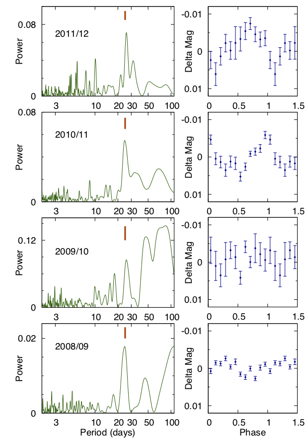
LHS 1815 was also observed by WASP-South over the period of 2008 to 2012 for a typical duration of 150 days in each year. WASP-South is an array of 8 cameras combining 200-mm f/1.8 lenses with 2k $\times$ 2k CCDs and observing with a broad-band filter giving a 400-700 nm bandpass (Pollacco et al., 2006). Each visible field was monitored with a cadence of $\sim$ 15 mins on every clear night, accumulating 50,000 data points on LHS 1815. The light curves from each observing season were searched for rotational modulations using the methods described in Maxted et al. (2011). For LHS 1815, we found a persistent modulation with a period of 24.9 $\pm$ 1.1 d with an amplitude of 2 to 8 mmag (Figure 9) and a false-alarm probability below 1%. This is consistent with the signal found in the TESS data, and confirms that the signal is likely caused by rotation as it is persistent for multiple years. Future TESS data to be obtained during the TESS Extended Mission will allow better identification to the correct rotation period of this target.

To assess stellar activity levels spectroscopically, we also extracted the chromatic index (CRX) and differential line width (dLW) indicators from the HARPS spectra using the publicly available SpEctrum Radial Velocity AnaLyser pipeline (SERVAL; Zechmeister et al., 2018). CRX summarizes the wavelength dependence of the RVs, and dLW is an alternative to the commonly used FWHM. The apparent lack of a significant correlation between the activity indicators and the RVs suggests that the RVs are not dominated by stellar activity (see Figure 10). The observed RV scatter is therefore likely caused primarily by the Doppler signal induced by the planet, consistent with the detection of a peak in the GLS periodogram at the frequency of the orbital period (Figure 3).

3.4 False Positive Analysis

As we previously discussed in Sec. 2.2, there are several scenarios which can cause a false positive — a transit-like signal in the TESS data that does not originate from a transiting star-planet system. We considered all data we have obtained and carefully ruled out the false positive scenarios below following Vanderspek et al. (2019), Crossfield et al. (2019), and Shporer et al. (2019).

1. Detection is caused by instrumental artifact:

We excluded this possibility because periodic transit signals were found in all 12 TESS sectors in which this target was observed, and in each sector the target was located at different CCD position.

2. LHS 1815 is a stellar eclipsing binary:

Our HARPS RV data did not show a significant RV variability at the few m s^-1 level. The $\rm 3\sigma$ mass upper-limit has also ruled out this scenario (Section 3.2).

3. Light from a nearby eclipsing binary is blended with LHS 1815:

Our two ground-based observations from LCO have cleared all nearby Gaia stars ( $\rm\Delta T\sim 8.7$ mag) within $\rm 2.5^{\prime}$ through the NEB analysis (Section 2.2). We did not find any obvious variation of those stars which indicates this cannot be the case. We have also made sure that the scatter in light curves of nearby stars is smaller than the expected eclipse depth given the brightness difference between the nearby star and the target.

4. Light from an unassociated distant eclipsing binary or a transiting planet system fully blended with LHS 1815 :

Thanks to the high proper motion of LHS 1815 ( $\rm\sim 760\ mas~{}yr^{-1}$ ), we can easily reject this scenario by checking images from other surveys decades ago. We did not see any other stars that are bright enough to cause the transit seen in TESS data at the current position of LHS 1815, as shown in Figure 2, thus this possibility is excluded.

5. LHS 1815 has a stellar binary companion on a wide orbit and that binary companion is the origin of the transit signal:

Photometric data from multiple sectors of TESS offered us an opportunity to deliver precise duration of transit ingress/egress and the time from first-to-third contact during the transit event. Assuming a symmetric light curve, we have

\frac{\rm\tau_{12}}{\rm\tau_{13}}=\frac{\rm t_{T}-t_{F}}{\rm t_{T}+t_{F}},

(1)

where $\rm t_{T}$ and $\rm t_{F}$ are the total and in-transit duration (2nd to 3rd contacts), respectively. Seager & Mallén-Ornelas (2003) gave the upper-limit of the radius ratio of the transiting planet:

\frac{\rm R_{p\_real}}{\rm R_{\star}}\leq\frac{\rm\tau_{12}}{\rm\tau_{13}}.

(2)

We constrained the relative flux drop if the signal is from an unresolved star:

\frac{\rm\Delta F}{f_{b}}=\left(\frac{\rm R_{p\_real}}{\rm R_{\star}}\right)^{2}\leq\left(\frac{\rm\tau_{12}}{\rm\tau_{13}}\right)^{2}=0.06\%.

(3)

Given the $\rm 3\sigma$ lower-limit on the exact transit depth from global modelling, the blended star has to contribute at least 50% of the total flux in the TESS aperture:

\frac{\rm\Delta F}{f_{s}+f_{b}}\geq 0.03\%;

(4)

\frac{f_{b}}{f_{s}+f_{b}}\geq 50\%,

(5)

where $f_{s}$ and $f_{b}$ are the source flux and blending flux. We excluded this scenario mainly based on the following reasons:
(1) According to this scenario the blending star is expected to have $\rm>50\%$ contribution to the TESS flux, but, Gaia and high resolution images show a non-detection of a nearby star at a few arcsec from the target.
(2) A star that is comparable in brightness to the target would make the spectrum appear double-lined but we do not see this phenomenon in the spectrum from HARPS.
(3) A star that is comparable in brightness to the target would cause the target to appear brighter for its distance. Since the distance is given by the Gaia DR2 parallax and $\rm T_{eff}$ is constrained by the SED, a blended star with comparable brightness will make the target appear too bright given its distance for a main sequence star, which is not the case.

4 Constraints from tidal evolution

We estimated the timescales for circularization and tidal decay using the equilibrium tide model from Hut (1981). We integrated the secularly averaged equations for the eccentricity and semimajor axis of the planet (namely, equations 9 and 10 from Hut 1981) using the midpoint method. We neglected the evolution of the planetary spin, since the spin angular momentum of the planet is too small with respect to the orbital angular momentum to affect the orbit significantly. Given the upper limit estimate for the mass $\mathrm{M}_{\mathrm{P}}$ of LHS 1815b and the intrinsic uncertainty of tidal efficiency parameters (the time-lag $\tau$ or the tidal quality factor $Q^{\prime}$ ), we have explored different tidal evolution models in the range $10\,\mathrm{s}<\tau<1000\,\mathrm{s}$ and $1\,\mathrm{M_{\oplus}}<\mathrm{M}_{\mathrm{P}}<6\,\mathrm{M_{\oplus}}$ . This range of time-lag is appropriate for planets with rocky composition (Socrates et al., 2012). For low tidal efficiency ( $\tau=10\,\mathrm{s}$ ), circularization takes longer than 10 Gyr regardless of the mass of the planet, while for high tidal efficiency ( $\tau=1000\,\mathrm{s}$ ) the planetary orbit is always completely circularized within 10 Gyr, with small planetary masses ( $\mathrm{M}_{\mathrm{P}}<3\,\mathrm{M_{\oplus}}$ ) circularizing within 1 Gyr. On the other hand, at moderate tidal efficiency ( $\tau=100\,\mathrm{s}$ ) the circularization timescale is sensible to the planetary mass. For $\tau=100\,\mathrm{s}$ and $\mathrm{M}_{\mathrm{P}}<3\,\mathrm{M_{\oplus}}$ the planetary orbit reaches $e\lesssim 0.05$ within 10 Gyr, while it retains some eccentricity for higher planetary masses ( $\mathrm{M}_{\mathrm{P}}>3\,\mathrm{M_{\oplus}}$ ).

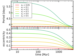
Figure 11 shows the evolution of orbital period and eccentricity of the planet, assuming $\mathrm{M}_{\mathrm{P}}=4.5\,\mathrm{M_{\oplus}}$ , a constant time-lag of $\tau=300\,\mathrm{s}$ , and an apsidal constant of $k_{A}=0.3$ , corresponding to a tidal quality factor of $Q^{\prime}=5\times 10^{2}$ . In the top panel of Figure 11 the planet has an initial period equal to the currently observed one, and different initial eccentricities. Initial eccentricities lower than 0.5 will be dissipated within about 5 Gyr, the lower the eccentricity, the longer the circularization time. However, as the eccentricity is dissipated, the orbital period decays so that the final period does not match the observed one. Specifically, the orbital period would mismatch the observed one within 100–200 Myr for all eccentricities $e\gtrsim 0.05$ .

In the bottom panel of Figure 11 we show the evolution for different initial periods so that the final period after circularization matches the present one. By 5 Gyr all the periods have reached the final value of $3.81433$ days with $e\lesssim 0.05$ . If the system was younger than 5 Gyr, it would not have time to circularize unless the initial eccentricity was $e\lesssim 0.1$ . Alternatively, it might be argued that the planet has not circularized yet. However, as shown by the top panel of Figure 11, any residual eccentricity higher than $0.05$ at $3.81433$ days would make the planet decay within $100$ Myr.

Ultimately, constraints on the age of the system would help narrowing down the possible range of eccentricities of the planet. If the system is very young ( $\rm{\sim}100\ Myr$ ), the eccentricity is largely uncertain since the planet must be currently undergoing tidal circularization. Conversely, if the system is old ( $>$ 5 Gyr), tidal circularization is mostly over and the eccentricity at present day is likely less than $0.05$ . Note also that the eccentricity could be excited by another undetected planet, a possibility that we have neglected in our analysis.

5 Thick-Disk Characteristics

We confirmed the thick-disk nature of LHS 1815 mainly on the basis of its kinematic information. In general, thick-disk stars are kinematically hotter (larger velocity dispersions) than stars that belong to the thin disk. We converted radial velocities and proper motions from Gaia DR2 to 3D velocities U, V and W⁹⁹9U, V, W are positive in the directions of Galactic center, Galactic rotation and the North Galactic Pole. using the distance of d = 29.87 $\pm$ 0.02 pc from our SED fit based on the method described in Johnson & Soderblom (1987). To relate the space velocities to the Local Standard of Rest (LSR), we adopted solar velocity components relative to the LSR ( $\rm U_{\odot}$ , $\rm V_{\odot}$ , $\rm W_{\odot}$ ) = ( $9.58$ , $10.52$ , $7.01$ ) km s^-1 obtained by LAMOST (Tian et al., 2015). We determined the three-dimensional Galactic space motion of ( $\rm U_{LSR}$ , $\rm V_{LSR}$ , $\rm W_{LSR}$ ) = ( $-34.34\pm 0.04$ , $-71.47\pm 0.22$ , $76.26\pm 0.14$ ) km s^-1.

To judge which stellar component LHS 1815 belongs to, we employed the kinematical criteria first mentioned in Bensby et al. (2003) by assuming the Galactic space velocities $\rm U_{LSR}$ , $\rm V_{LSR}$ , and $\rm W_{LSR}$ of the stellar populations have Gaussian distributions:

f=\rm k\times exp(-\frac{\rm{U_{LSR}}^{2}}{2{\sigma_{U}}^{2}}-\frac{\rm{(V_{LSR}-V_{asym})}^{2}}{2{\sigma_{V}}^{2}}-\frac{\rm{W_{LSR}}^{2}}{2{\sigma_{W}}^{2}}),

(6)

where

\rm k=\frac{1}{(2\pi)^{3/2}\sigma_{U}\sigma_{V}\sigma_{W}}

(7)

is a normalization constant, $\rm\sigma_{U}$ , $\rm\sigma_{V}$ and $\rm\sigma_{W}$ represent velocity dispersion for 3D velocity components while $\rm V_{asym}$ is the asymmetric drift. We applied related parameters from Bensby et al. (2014) for solar-neighborhood stars and calculated relative probability $\rm P_{thick}/P_{thin}$ for LHS 1815 and other TESS planet host stars to be in the thick (TD) and thin disks (D). Figure 12 shows the corresponding Toomre plot. We considered stars with $\rm P_{thick}/P_{thin}>10$ to be in the thick disk while stars in between ( $\rm 0.1<P_{thick}/P_{thin}<10$ ) are ambiguous to judge. Up to now, TESS has detected five planet host stars located in the in-between region: TOI 118 (Esposito et al., 2019), TOI 144 (Huang et al., 2018b), TOI 172 (Rodriguez et al., 2019), TOI 186 (Trifonov et al., 2019; Dragomir et al., 2019) and TOI 197 (Huber et al., 2019). Table 4 lists their relative probabilities and none of them show clear-cut thick-disk probability. However, we obtained a large relative probability ( $\rm P_{thick}/P_{thin}$ = 6482) for LHS 1815, indicating it is very likely a thick-disk star. Soubiran et al. (2003) showed that thick-disk stars tend to have much lower metallicity than thin-disk stars. Therefore, our metallicity measurement $\rm[Fe/H]=-0.12\pm 0.09$ , based on the HARPS spectra, is consistent a thick-disk origin.

Table 4: Relative probability for TESS stars with ambiguous separation between thick and thin components

Star	$\rm P_{thick}/P_{thin}$
TOI-118	4.825
TOI-144	0.127
TOI-172	1.430
TOI-186	0.125
TOI-197	0.292
LHS 1815	6482

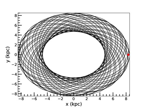
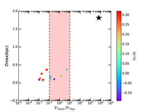
In order to gain insight into further dynamical information, we used galpy (Bovy, 2015) to simulate the orbit of LHS 1815. We initialized the orbit using RA, DEC, star distance, proper motions in two directions and heliocentric line-of-sight velocity. We integrated the orbit from t = 0 to t = 10 Gyr in a general potential: MWPotential2014, saving the orbit for 10000 steps. The orbital result of LHS 1815 is shown in Figure 13. The maximal height $\rm Z_{max}$ of LHS 1815 above the plane of the orbit is 1.8 kpc, consistent with our thick disk conclusion before. For comparison, we plot $\rm Z_{max}$ and the relative probability of all TESS planet host stars in Figure 14. It is clear that the five TOI stars located in the region between the thin and thick disks are more likely to belong to the Galactic thin disk given their small $\rm Z_{max}$ . LHS 1815 is moving upwards currently; an additional orbital integration analysis shows that LHS 1815 will spend $\rm\sim 14\ Myr$ to first reach 1 kpc above the Galactic plane. Before LHS 1815 reaches the plane again, we have a probability about 33% to see it ( $\rm Z<1kpc$ ).

Table 5: Final parameters of LHS 1815b

Parameter	Value	Prior
Fitting parameters
$\rm P_{orb}$ (days)	$3.81433\pm 0.00003$	$\mathcal{N}^{[1]}$ (3.814 , $0.1^{2}$ )
$\rm T_{C}$ (BJD)	$2458327.4161\pm 0.0016$	$\mathcal{N}$ (2458327.4 , 0.1)
$\rm R_{P}/R_{\star}$	$0.0199\pm 0.0009$	$\mathcal{U}^{[2]}$ (0.005 , 0.05)
$\rm a/R_{\star}$	$17.403\pm 2.816$	$\mathcal{N}$ (16 , 3)
$i$ (deg)	$88.125\pm 1.113$	$\mathcal{U}$ (0 , 180)
$\rm q_{1}$	$0.26\pm 0.19$	$\mathcal{U}$ (0 , 1)
$\rm q_{2}$	$0.35\pm 0.26$	$\mathcal{U}$ (0 , 1)
$K$ ( $\rm m\ s^{-1}$ )	$2.7\pm 1.0$	$\mathcal{U}$ (0 , 10)
$\rm\gamma_{rel}$ ( $\rm m\ s^{-1}$ )	$-0.38\pm 0.64$	$\mathcal{U}$ (-10 , 10)
$\rm\sigma_{J}$ ( $\rm m\ s^{-1}$ )	$2.0\pm 0.6$	$\mathcal{J}^{[3]}$ (0.1 , 10)
$e$	0	Fixed
$\omega$ (deg)	90	Fixed
Derived parameters
$\rm R_{P}$ ( $\rm R_{\oplus}$ )	$1.088\pm 0.064$
$\rm M_{P}$ ( $\rm M_{\oplus}$ )^[4]	$4.2\pm 1.5$
$\rm a$ (AU)	$0.0404\pm 0.0094$
$\rm T_{eq}$ (K)^[5]	$617\pm 84$

1

[1] $\mathcal{N}$ ( $\mu\ ,\ \sigma$ ) means a normal prior with mean $\mu$ and standard deviation $\sigma$ .
2

[2] $\mathcal{U}$ (a , b) stands for a uniform prior ranging from a to b.
3

[3] $\mathcal{J}$ (a , b) stands for a Jeffrey’s prior with the same limits.
4

[4] This is not a statistically significant measurement. $3\sigma$ mass upper-limit is $\rm 8.7\ M_{\oplus}$ .
5

[5] Suppose albedo = 0 and there is no heat distribution here.

6 Discussion and Conclusion

LHS 1815b is the first thick-disk planet detected by TESS. It has a radius of $\rm R_{P}=1.088\pm 0.064\ R_{\oplus}$ and a mass of $\rm M_{P}=4.2\pm 1.5\ M_{\oplus}$ . The proximity of LHS 1815 and its interesting kinematic features makes it a system worth further characterization.

6.1 Prospects on Future Follow-up Observations

Given the brightness of LHS 1815, it is an attractive target for precise RV measurements with high resolution spectroscopy facilities. Those will lead to precise mass measurement of the transiting planet and will be used to search for other planets in the system. A precise planet mass will give an improved estimate of the suitability of LHS 1815b for atmospheric characterization. The rotation period of LHS 1815 is well separated from the orbital period of the planet, making it possible to smooth out the effect from stellar activity.

In addition, since LHS 1815 is nearby ( $29.87\pm 0.02$ pc), future release of Gaia time series astrometry can be used to look for massive objects (massive planets and brown dwarfs) at wide orbits, with potential partial overlap with objects on orbits that radial velocities will be sensitive to.

To evaluate the feasibility of high-quality atmospheric characterization by JWST (Gardner et al., 2006), we first use the Transmission Spectroscopy Metric (TSM) formulated by Kempton et al. (2018) and we find $\rm TSM\sim 2.5^{+3.8}_{-1.3}$ for LHS 1815. Kempton et al. (2018) recommends that planets with $\rm TSM>10$ for $\rm R_{p}<1.5\ R_{\oplus}$ are high-quality atmospheric characterization targets. The relatively large TSM uncertainty due to the weak constraint on the planet mass results in unclear determination on whether LHS 1815 is a good (although unlikely the best) target for transmission spectroscopy studies. In addition, we compute the Emission Spectroscopy Metric (ESM) for LHS 1815 and we find $\rm ESM\sim 1.9^{+1.0}_{-0.8}$ . Given the recommended threshold $\rm ESM=7.5$ from Kempton et al. (2018), LHS 1815 is not an ideal target for emission spectroscopy researches, either.

6.2 Planet Formation Efficiency in Thin and Thick Disk?

A followup statistical work about the planet formation efficiency in the thin and thick disk is ongoing (Gan et al., in prep) based on all TESS planet candidates detected in the Southern Hemisphere. The current TESS survey for the Northern Hemisphere will be an excellent opportunity to further examine this subject. First, TESS focuses on finding exoplanets around nearby bright stars and most TOIs have precise astrometry and RV measurement from Gaia DR2, which can determine their thin, thick and halo origin. Second, LAMOST (The Large Sky Area Multi-Object Fiber Spectroscopic Telescope, Cui et al. 2012) can provide chemical element abundance measurements to check the classification for a large number of stars.

We emphasize that here we only consider the formation efficiency for nearby bright stars. Faint stars ( $\rm G>13$ mag) at relatively large distances may not have RV measurement from Gaia DR2, leading to a poor separation between thin and thick disks. Future surveys such as DESI (DESI Collaboration et al., 2016) and spectroscopic observations from SPIRou (Challita et al., 2018) shall remedy this situation.

7 Acknowledgement

We thank Sharon Xuesong Wang, Chao Liu and Weicheng Zang for their insights and advice. Funding for the TESS mission is provided by NASA’s Science Mission directorate. This work is partly supported by the National Science Foundation of China (Grant No. 11390372 and 11761131004 to SM and GTJ). We acknowledge the use of TESS Alert data from pipelines at the TESS Science Office and at the TESS Science Processing Operations Center. Resources supporting this work were provided by the NASA High-End Computing (HEC) Program through the NASA Advanced Supercomputing (NAS) Division at Ames Research Center for the production of the SPOC data products. J.G.W. is supported by a grant from the John Templeton Foundation. The opinions expressed in this publication are those of the authors and do not necessarily reflect the views of the John Templeton Foundation. C.Z. is supported by a Dunlap Fellowship at the Dunlap Institute for Astronomy & Astrophysics, funded through an endowment established by the Dunlap family and the University of Toronto. Some of the observations in the paper made use of the High-Resolution Imaging instrument Zorro at Gemini-South). Zorro was funded by the NASA Exoplanet Exploration Program and built at the NASA Ames Research Center by Steve B. Howell, Nic Scott, Elliott P. Horch, and Emmett Quigley. This research has made use of the Exoplanet Follow-up Observation Program website, which is operated by the California Institute of Technology, under contract with the National Aeronautics and Space Administration under the Exoplanet Exploration Program. This paper includes data collected by the TESS mission, which are publicly available from the Mikulski Archive for Space Telescopes (MAST). This research made use of observations from the LCO network, WASP-South and ESO: 3.6m (HARPS).

References

Adibekyan et al. (2011) Adibekyan, V. Z., Santos, N. C., Sousa, S. G., & Israelian, G. 2011, A&A, 535, L11
Adibekyan et al. (2013) Adibekyan, V. Z., Figueira, P., Santos, N. C., et al. 2013, A&A, 554, A44
Anglada-Escudé & Butler (2012) Anglada-Escudé, G., & Butler, R. P. 2012, ApJS, 200, 15
Baglin et al. (2006) Baglin, A., Auvergne, M., Boisnard, L., et al. 2006, in 36th COSPAR Scientific Assembly, Vol. 36, 3749
Bakos et al. (2004) Bakos, G., Noyes, R. W., Kovács, G., et al. 2004, PASP, 116, 266
Barentsen et al. (2019) Barentsen, G., Hedges, C., Vinícius, Z., et al. 2019, KeplerGO/lightkurve: Lightkurve v1.0b29, doi:10.5281/zenodo.2565212
Bensby et al. (2003) Bensby, T., Feltzing, S., & Lundström, I. 2003, A&A, 410, 527
Bensby et al. (2005) Bensby, T., Feltzing, S., Lundström, I., & Ilyin, I. 2005, A&A, 433, 185
Bensby et al. (2014) Bensby, T., Feltzing, S., & Oey, M. S. 2014, A&A, 562, A71
Borucki et al. (2010) Borucki, W. J., Koch, D., Basri, G., et al. 2010, Science, 327, 977
Bouchy et al. (2010) Bouchy, F., Hebb, L., Skillen, I., et al. 2010, A&A, 519, A98
Bovy (2015) Bovy, J. 2015, ApJS, 216, 29
Brown (2003) Brown, T. M. 2003, ApJ, 593, L125
Brown et al. (2013) Brown, T. M., Baliber, N., Bianco, F. B., et al. 2013, PASP, 125, 1031
Buser et al. (1999) Buser, R., Rong, J., & Karaali, S. 1999, A&A, 348, 98
Campante et al. (2015) Campante, T. L., Barclay, T., Swift, J. J., et al. 2015, ApJ, 799, 170
Challita et al. (2018) Challita, Z., Reshetov, V., Baratchart, S., et al. 2018, in Society of Photo-Optical Instrumentation Engineers (SPIE) Conference Series, Vol. 10702, Ground-based and Airborne Instrumentation for Astronomy VII, 1070262
Claret (2018) Claret, A. 2018, A&A, 618, A20
Collins et al. (2017) Collins, K. A., Kielkopf, J. F., Stassun, K. G., & Hessman, F. V. 2017, AJ, 153, 77
Crossfield et al. (2019) Crossfield, I. J. M., Waalkes, W., Newton, E. R., et al. 2019, ApJ, 883, L16
Cui et al. (2012) Cui, X.-Q., Zhao, Y.-H., Chu, Y.-Q., et al. 2012, Research in Astronomy and Astrophysics, 12, 1197
Cutri et al. (2003) Cutri, R. M., Skrutskie, M. F., van Dyk, S., et al. 2003, 2MASS All Sky Catalog of point sources.
Deeg et al. (2009) Deeg, H. J., Gillon, M., Shporer, A., et al. 2009, A&A, 506, 343
Deming et al. (2015) Deming, D., Knutson, H., Kammer, J., et al. 2015, ApJ, 805, 132
DESI Collaboration et al. (2016) DESI Collaboration, Aghamousa, A., Aguilar, J., et al. 2016, arXiv e-prints, arXiv:1611.00036
Dragomir et al. (2019) Dragomir, D., Teske, J., Günther, M. N., et al. 2019, ApJ, 875, L7
Espinoza et al. (2016) Espinoza, N., Brahm, R., Jordán, A., et al. 2016, ApJ, 830, 43
Esposito et al. (2019) Esposito, M., Armstrong, D. J., Gandolfi, D., et al. 2019, A&A, 623, A165
Foreman-Mackey et al. (2013) Foreman-Mackey, D., Hogg, D. W., Lang, D., & Goodman, J. 2013, PASP, 125, 306
Fuhrmann (2008) Fuhrmann, K. 2008, MNRAS, 384, 173
Fuhrmann & Bernkopf (2008) Fuhrmann, K., & Bernkopf, J. 2008, MNRAS, 384, 1563
Fulton et al. (2018) Fulton, B. J., Petigura, E. A., Blunt, S., & Sinukoff, E. 2018, PASP, 130, 044504
Gaia Collaboration et al. (2018) Gaia Collaboration, Babusiaux, C., van Leeuwen, F., et al. 2018, A&A, 616, A10
Gardner et al. (2006) Gardner, J. P., Mather, J. C., Clampin, M., et al. 2006, Space Sci. Rev., 123, 485
Gilmore & Reid (1983) Gilmore, G., & Reid, N. 1983, MNRAS, 202, 1025
Gonzalez (1997) Gonzalez, G. 1997, MNRAS, 285, 403
Hippke & Heller (2019) Hippke, M., & Heller, R. 2019, A&A, 623, A39
Hirano et al. (2018) Hirano, T., Dai, F., Livingston, J. H., et al. 2018, AJ, 155, 124
Howell et al. (2011) Howell, S. B., Everett, M. E., Sherry, W., Horch, E., & Ciardi, D. R. 2011, AJ, 142, 19
Howell et al. (2014) Howell, S. B., Sobeck, C., Haas, M., et al. 2014, PASP, 126, 398
Huang et al. (2018a) Huang, C. X., Shporer, A., Dragomir, D., et al. 2018a, ArXiv e-prints, arXiv:1807.11129
Huang et al. (2018b) Huang, C. X., Burt, J., Vanderburg, A., et al. 2018b, ApJ, 868, L39
Huber et al. (2019) Huber, D., Chaplin, W. J., Chontos, A., et al. 2019, AJ, 157, 245
Hut (1981) Hut, P. 1981, A&A, 99, 126
Jenkins (2002) Jenkins, J. M. 2002, ApJ, 575, 493
Jenkins et al. (2017) Jenkins, J. M., Tenenbaum, P., Seader, S., et al. 2017, Kepler Data Processing Handbook: Transiting Planet Search, Kepler Science Document
Jenkins et al. (2016) Jenkins, J. M., Twicken, J. D., McCauliff, S., et al. 2016, in Proc. SPIE, Vol. 9913, Software and Cyberinfrastructure for Astronomy IV, 99133E
Johnson & Soderblom (1987) Johnson, D. R. H., & Soderblom, D. R. 1987, AJ, 93, 864
Jurić et al. (2008) Jurić, M., Ivezić, Ž., Brooks, A., et al. 2008, ApJ, 673, 864
Kempton et al. (2018) Kempton, E. M. R., Bean, J. L., Louie, D. R., et al. 2018, PASP, 130, 114401
Kreidberg (2015) Kreidberg, L. 2015, PASP, 127, 1161
Livingston et al. (2018) Livingston, J. H., Dai, F., Hirano, T., et al. 2018, AJ, 155, 115
Mann et al. (2015) Mann, A. W., Feiden, G. A., Gaidos, E., Boyajian, T., & von Braun, K. 2015, ApJ, 804, 64
Mann et al. (2019) Mann, A. W., Dupuy, T., Kraus, A. L., et al. 2019, ApJ, 871, 63
Maxted et al. (2011) Maxted, P. F. L., Anderson, D. R., Collier Cameron, A., et al. 2011, PASP, 123, 547
Mayor et al. (2003) Mayor, M., Pepe, F., Queloz, D., et al. 2003, The Messenger, 114, 20
McTier & Kipping (2019) McTier, M. A. S., & Kipping, D. M. 2019, MNRAS, 489, 2505
Mermilliod (2006) Mermilliod, J. C. 2006, VizieR Online Data Catalog, II/168
Murdoch et al. (1993) Murdoch, K. A., Hearnshaw, J. B., & Clark, M. 1993, ApJ, 413, 349
Neves et al. (2009) Neves, V., Santos, N. C., Sousa, S. G., Correia, A. C. M., & Israelian, G. 2009, A&A, 497, 563
Pecaut & Mamajek (2013) Pecaut, M. J., & Mamajek, E. E. 2013, ApJS, 208, 9
Perger et al. (2017) Perger, M., García-Piquer, A., Ribas, I., et al. 2017, A&A, 598, A26
Pollacco et al. (2006) Pollacco, D. L., Skillen, I., Collier Cameron, A., et al. 2006, PASP, 118, 1407
Prochaska et al. (2000) Prochaska, J. X., Naumov, S. O., Carney, B. W., McWilliam, A., & Wolfe, A. M. 2000, AJ, 120, 2513
Rasmussen & Williams (2005) Rasmussen, C. E., & Williams, C. K. I. 2005, Gaussian Processes for Machine Learning (Adaptive Computation and Machine Learning) (The MIT Press)
Reddy et al. (2006) Reddy, B. E., Lambert, D. L., & Allende Prieto, C. 2006, MNRAS, 367, 1329
Reid et al. (2007) Reid, I. N., Turner, E. L., Turnbull, M. C., Mountain, M., & Valenti, J. A. 2007, ApJ, 665, 767
Ricker et al. (2014) Ricker, G. R., Winn, J. N., Vanderspek, R., et al. 2014, in Proc. SPIE, Vol. 9143, Space Telescopes and Instrumentation 2014: Optical, Infrared, and Millimeter Wave, 914320
Rodriguez et al. (2019) Rodriguez, J. E., Quinn, S. N., Huang, C. X., et al. 2019, AJ, 157, 191
Sartoretti et al. (2018) Sartoretti, P., Katz, D., Cropper, M., et al. 2018, A&A, 616, A6
Seager & Mallén-Ornelas (2003) Seager, S., & Mallén-Ornelas, G. 2003, ApJ, 585, 1038
Shporer et al. (2019) Shporer, A., Collins, K. A., Astudillo-Defru, N., et al. 2019, arXiv e-prints, arXiv:1912.05556
Skrutskie et al. (2006) Skrutskie, M. F., Cutri, R. M., Stiening, R., et al. 2006, AJ, 131, 1163
Smith et al. (2012) Smith, J. C., Stumpe, M. C., Van Cleve, J. E., et al. 2012, PASP, 124, 1000
Socrates et al. (2012) Socrates, A., Katz, B., & Dong, S. 2012, ArXiv e-prints, arXiv:1209.5724
Soubiran et al. (2003) Soubiran, C., Bienaymé, O., & Siebert, A. 2003, A&A, 398, 141
Sozzetti et al. (2007) Sozzetti, A., Torres, G., Charbonneau, D., et al. 2007, ApJ, 664, 1190
Stassun et al. (2017) Stassun, K. G., Collins, K. A., & Gaudi, B. S. 2017, AJ, 153, 136
Stassun et al. (2018a) Stassun, K. G., Corsaro, E., Pepper, J. A., & Gaudi, B. S. 2018a, AJ, 155, 22
Stassun & Torres (2016) Stassun, K. G., & Torres, G. 2016, AJ, 152, 180
Stassun & Torres (2018) —. 2018, ApJ, 862, 61
Stassun et al. (2018b) Stassun, K. G., Oelkers, R. J., Pepper, J., et al. 2018b, AJ, 156, 102
Stassun et al. (2019) Stassun, K. G., Oelkers, R. J., Paegert, M., et al. 2019, AJ, 158, 138
Stumpe et al. (2014) Stumpe, M. C., Smith, J. C., Catanzarite, J. H., et al. 2014, PASP, 126, 100
Stumpe et al. (2012) Stumpe, M. C., Smith, J. C., Van Cleve, J. E., et al. 2012, PASP, 124, 985
Sullivan et al. (2015) Sullivan, P. W., Winn, J. N., Berta-Thompson, Z. K., et al. 2015, ApJ, 809, 77
Tian et al. (2015) Tian, H.-J., Liu, C., Carlin, J. L., et al. 2015, ApJ, 809, 145
Tokovinin (2018) Tokovinin, A. 2018, PASP, 130, 035002
Trifonov et al. (2019) Trifonov, T., Rybizki, J., & Kürster, M. 2019, A&A, 622, L7
Vanderspek et al. (2019) Vanderspek, R., Huang, C. X., Vanderburg, A., et al. 2019, ApJ, 871, L24
Wright et al. (2010) Wright, E. L., Eisenhardt, P. R. M., Mainzer, A. K., et al. 2010, AJ, 140, 1868
Yee et al. (2017) Yee, S. W., Petigura, E. A., & von Braun, K. 2017, ApJ, 836, 77
Zechmeister & Kürster (2009) Zechmeister, M., & Kürster, M. 2009, A&A, 496, 577
Zechmeister et al. (2018) Zechmeister, M., Reiners, A., Amado, P. J., et al. 2018, A&A, 609, A12