Leveraging (Biased) Information: Multi-armed Bandits with Offline Data
Abstract
We leverage offline data to facilitate online learning in stochastic multi-armed bandits. The probability distributions that govern the offline data and the online rewards can be different. Without any non-trivial upper bound on their difference, we show that no non-anticipatory policy can out-perform the UCB policy by (Auer et al. 2002), even in the presence of offline data. In complement, we propose an online policy MIN-UCB, which outperforms UCB when a non-trivial upper bound is given. MIN-UCB adaptively chooses to utilize the offline data when they are deemed informative, and to ignore them otherwise. MIN-UCB is shown to be tight in terms of both instance independent and dependent regret bounds. Finally, we corroborate the theoretical results with numerical experiments.
1 Introduction
Multi-armed bandit problem (MAB) is a classical model in sequential decision-making. In traditional models, online learning is initialized with no historical dataset. However, in many real world scenarios, historical datasets related to the underlying model exist before online learning begins. Those datasets could be beneficial to online learning. For instance, when a company launch a new product in Singapore, past sales data in the US could be of relevance. This prompts an intriguing question: Can we develop an approach that effectively utilizes offline data, and subsequently learns under bandit feedback? Such approaches carry significant allure, as they potentially reduce the amount of exploration in the learning process. Nevertheless, it is too strong and impractical to assume that the historical dataset and the online model follow the same probability distribution, given the ubiquity of distributional shifts. Therefore, it is desirable to design an adaptive policy that reaps the benefit of offline data if they closely match the online model, while judiciously ignores the offline data and learns from scratch otherwise.
Motivated by the above discussions, we consider a stochastic multi-armed bandit model with possibly biased offline dataset. The entire event horizon consists of a warm-start phase, followed by an online phase whereby decision making occurs. During the warm-start phase, the DM receives an offline dataset, consisting of samples governed by a latent probabiltiy distribution . The subsequent online phase is the same as standard multi-armed bandit model, except that the offline dataset can be incorporated in decision making. The random online rewards are governed by another latent probabiltiy distribution . The DM aims to maximize the total cumulative reward earned, or equivalently minimize the regret, during the online phase.
Intuitively, when , are “far apart”, the DM should conduct online learning from scratch and ignore the offline dataset. For example, the vanilla UCB policy by (Auer et al., 2002) incurs expected regret at most
| (1) |
where is the length of online phase, and is the difference between the expected reward of an optimal arm and arm (also see Section 2). The bound (1) holds for all , . In contrary, when , are “sufficiently close”, the DM should incorporate the offline data into online learning and avoid unnecessary exploration. For example, when , HUCB1 (Shivaswamy & Joachims, 2012) and MonUCB (Banerjee et al., 2022) incur expected regret at most
| (2) |
where is the number of offline samples on arm . (2) is a better regret bound than (1). However, (2) only holds when . The above inspires the following question:
(Q) Can the DM outperform the vanilla UCB, i.e. achieves a better regret bound than (1) when , while retains the regret bound (1) for general ?
The answer to (Q) turns out to be somewhat mixed. Our novel contributions shed light on (Q) as follows:
Impossibility Result. We show in Section 3 that no non-anticipatory policy can achieve the aim in (Q). Even with an offline dataset, no non-anticipatory policy can outperform the vanilla UCB without any additional knowledge or restriction on the difference between .
Algorithm design and analysis. To bypass the impossibility result, we endow the DM with an auxiliary information dubbed valid bias bound , which is an information additional to the offline dataset. The bound serves as an upper bound on the difference between and . We propose the MIN-UCB policy, which achieves a strictly better regret bound than (1) when are “sufficiently close”. In particular, our regret bound reduces to (2) if the DM knows . We provide both instance dependent and independent regret upper bounds on MIN-UCB, and we show their tightness by providing the corresponding regret lower bounds. Our analysis also pins down the precise meaning of “far apart” and “sufficientlly close” in the above discussion. The design and analysis of MIN-UCB are provided in Section 4.
In particular, when , our analysis provide two novel contributions. Firstly, we establish the tightness of the instance dependent bound (2). Secondly, we establish a pair of instance independent regret upper and lower bounds, which match each other up to a logarithmic factor. MIN-UCB is proved to achieve the upper bound when . Both the upper and lower bounds are novel in the literature, and we show that the optimal regret bound involves the optimum of a novel linear program.
1.1 Related Works
Multi-armed bandits with offline data has been studied in multiple works. (Shivaswamy & Joachims, 2012; Banerjee et al., 2022) are the most relevant works, focusing on the special case of . They only provide instance dependent regret upper bound, while we both instance dependent and independent bounds. Online learning with offline data under is also studied in dynamic pricing settings (Bu et al., 2020) and reinforcement learning settings (Hao et al., 2023; Wagenmaker & Pacchiano, 2023), as well as when historical data are sequentially provided (Gur & Momeni, 2022), or provided as clustered data (Bouneffouf et al., 2019; Ye et al., 2020; Tennenholtz et al., 2021). (Zhang et al., 2019) is another closely related work on contextual bandits that allows . We provide more discussions on it in Appendix A.1.
Bayesian policies, such as the Thompson sampling policy (TS), are popular for incorporating offline data into online learning. When the online and offline reward distributions are identical, offline data can be used to construct well-specified priors, which enables better regret bounds than (Russo & Van Roy, 2014; Russo & Roy, 2016; Liu & Li, 2016) when the offline data size increases. By contrast, (Liu & Li, 2016; Simchowitz et al., 2021) show that the TS initialized with mis-specified priors generally incurs worse regret bounds than state-of-the-art online policies without any offline data. Our work focuses on an orthogonal issue of deciding whether to incorporate the possibly biased offline data in online learning.
Our problem model closely relates to machine learning under domain shift. (Si et al., 2023) investigates a offline policy learning problem using historical data on contextual bandits under changing environment from a distributionally robust optimization perspective. (Chen et al., 2022) studies a variant in RL context, and their policy is also endowed with an upper bound on the distributional drift between offline and online models. We provide more discussion in Appendix A.3. Numerous research works consider the issue of distributional drift in supervised learning (Crammer et al., 2008; Mansour et al., 2009; Ben-David et al., 2010) and stochastic optimization (Besbes et al., 2022).
Our work is related to research on online learning with advice, which focuses on improving performance guarantees with hints or predictions. Indeed, our offline dataset could serve as a hint to an online learner. A variety of results are derived in multi-armed bandits (Wei & Luo, 2018), linear bandits (Cutkosky et al., 2022), contextual bandits (Wei et al., 2020b), and full feedback settings (Steinhardt & Liang, 2014; Rakhlin & Sridharan, 2013a, b). These works do not apply in our setting, since they do not consider refining instance dependent bounds. We provide more discussions in Appendix A.2. Our theme of whether to utilize the potentially biased offline data is related to online model selection, studied in (Agarwal et al., 2017; Pacchiano et al., 2020; Lee et al., 2021; Cutkosky et al., 2021; Pacchiano et al., 2023). While these works take a black-box approach, we tailor-make our decision making on whether to utilize offline data with a novel UCB algorithm and the auxilliary input , and the latter is not studied in the abovemoentioned works.
Notation. We denote as the Gaussian disribution with mean and variance 1. We abbreviate identically and independently distributed as “i.i.d.”. The relationship means that the random variable follows the probability distribution .
2 Model
We consider a stochastic -armed bandit model with possibly biased offline data. Denote as the set of arms. The event horizon consists of a warm-start phase, then an online phase. During the warm-start phase, the DM receive a collection of i.i.d. samples, denoted , for each . We postulate that , the offline reward distribution on arm .
The subsequent online phase consists of time steps. For time steps , the DM chooses an arm to pull, which gives the DM a random reward . Pulling arm in the online phase generates a random reward , dubbed the online reward distribution on arm . We emphasize that needs not be the same as . Finally, the DM proceeds to time step , or terminates when .
The DM chooses arms with a non-anticipatory policy . The function maps the observations collected at the end of , to an element in . The quantity is the probability of , conditioned on under policy . While our proposed algorithms are deterministic, i.e. always, we allow randomized policies in our regret lower bound results. The policy could utilize , which provides a potentially biased estimate to the online model since we allow .
Altogether, the underlying instance is specified by the tuple , where . The DM only knows and , but not and , at the start of the online phase. For every , we assume that both are 1-subGaussian, which is also known to the DM. For , denote , and . We do not have any boundedness assumptions on .
The DM aims to maximize the total reward earned in the online phase. We quantify the performance guarantee of the DM’s non-anticipatory policy by its regret. Define , and denote for each . The DM aims to design a non-anticipatory policy minimize the regret
| (3) |
despite the uncertainty on . While (3) involves only but not , the choice of is influenced by both the offline data and the online data .
As mentioned in the introduction and detailed in the forthcoming Section 3, the DM cannot outperform the vanilla UCB policy with a non-anticipatory policy. Rather, the DM requires information additional to the offline dataset and a carefully designed policy. We consider the following auxiliary input in our algorithm design.
Auxiliary input: valid bias bound. We say that is a valid bias bound on an instance if
| (4) |
In our forthcoming policy MIN-UCB, the DM is endowed the auxiliary input in addition to the offline dataset before the online phase begins. The quantity serves as an upper bound on the amount of distributional shift from to . The condition (4) always holds in the trivial case of , which is when the DM has no additional knowledge. By contrast, when , the DM has a non-trivial knowledge on the difference .
The knowledge on an upper bound such as is in line with the model assumptions in research works on learning under distributional shift. Similar upper bounds are assumed in the contexts of supervised learning (Crammer et al., 2008), stochastic optimization (Besbes et al., 2022), offline policy learning on contextual bandits (Si et al., 2023), multi-task bandit learning (Wang et al., 2021), for example. Methodologies for constructing such upper bounds are provided in some literature. For instance, (Blanchet et al., 2019) designs an approach based on several machine learning estimators, such as LASSO. (Si et al., 2023) provides some managerial insights on how to construct them empirically. (Chen et al., 2022) constructs them through cross-validation, and implement it in a case study.
3 An Impossibility Result
We illustrate the impossibility result with two instances . The instances share the same and . However, differ in their respective reward distributions , , and have different optimal arms. Consider a fixed but arbitrary . Instance has well-aligned reward distributions , where
Note that . In , an offline dataset provides useful hints on arm 1 being optimal. For example, given where , the existing policies H-UCB and MonUCB achieve an expected regret (see Equation (2)) at most
which strictly outperforms the vanilla UCB policy that incurs expected regret . Despite the apparent improvement, the following claim shows that any non-anticipatory policy (not just H-UCB or MonUCB) that outperforms the vanilla UCB on would incur a larger regret than the vanilla UCB on a suitably chosen .
Proposition 3.1.
Let be arbitrary. Consider an arbitrary non-anticipatory policy (which only possesses the offline dataset but not the auxiliary input ) satisfies on instance , where , is an absolute constant, and the horizon is so large that . Set in the instance as
The following inequality holds:
| (5) | ||||
Proposition 3.1 is proved in Appendix section C.2. We first remark on . Different from , arm 2 is the optimal arm in . Thus, the offline data from provides the misleading information that arm 1 has a higher expected reward. In addition, note that , so the offline datasets in instances are identically distributed. The proposition suggests that no non-anticipatory policy can simultaneously (i) establish that is useful for online learning in to improve upon the UCB policy, (ii) establish that is to be disregarded for online learning in to match the UCB policy, negating the short-lived conjecture in (Q).
Lastly, we allow to be arbitrary. In the most informative case of , meaning that the DM knows in respectively, the DM still cannot achieve (i, ii) simultaneously. Indeed, the assumed improvement limits the number of pulls on arm 2 in during the online phase. We harness this property to construct an upper bound on the KL divergence between on online dynamics on , , which in turns implies the DM cannot differentiate between under policy . The KL divergence argument utilizes a chain rule (see Appendix C.1) on KL divergence adapted to our setting.
4 Design and Analysis of MIN-UCB
After the impossibility result, we present our MIN-UCB policy in Algorithm 1. MIN-UCB follows the optimism-in-face-of-uncertainty principle. At time , MIN-UCB sets as the UCB on . While follows (Auer et al., 2002), the construction of in (6) adheres to the following ideas that incorporates a valid bias bound , the auxiliary input.
| (6) |
| (7) |
In (6), the sample mean incorporates both online and offline data. Then, we inject optimism by adding , set in (7). The square-root term in (7) reflects the optimism in view of the randomness of the sample mean. The term in (7) injects optimism to correct the potential bias from the offline dataset. The correction requires the auxiliary input .
Finally, we adopt as the UCB when the bias bound is so small and the sample size is so large that . Otherwise, is deemed “far away” , and we follow the vanilla UCB. Our adaptive decisions on whether to incorporate offline data at each time step is different from the vanilla UCB policy that always ignores offline data, or from HUCB and MonUCB that always incorporate all offline data.
Lastly, we remark on . Suppose that the DM possesses no knowledge on additional to the offline dataset at the start of the online phase. Then, it is advisable to set for all , which specializes MIN-UCB to the vanilla UCB policy. Indeed, the theoretical impossibility result in Section 3 dashes out any hope for adaptively tuning in MIN-UCB with online data, in order to outperform the vanilla UCB. By contrast, when the DM has a non-trivial upper bound on , we show that can uniformly out-perform the vanilla UCB that direclty ignores the offline data.
We next embark on the analysis on MIN-UCB, by establishing instance dependent regret bounds in Section 4.1 and instance independent regret bounds in Section 4.3. Both sections relies on considering the following events of accurate estimations by . For each , define , where
While incorporates estimation error due to stochastic variations, additionally involves the potential bias of the offline data.
Lemma 4.1.
4.1 Instance Dependent Regret Bounds
Both our instance dependent regret upper and lower bounds depend on the following discrepancy measure
| (8) |
on an arm . Note that depends on both the valid bias bound and the model parameters By the validity of , we know that .
Theorem 4.2.
Consider policy MIN-UCB, which inputs a valid bias bound on the underlying instance and for . We have
| (9) |
where is over , and
| (10) |
Theorem 4.2 is proved in the Appendix B.2. We provide a sketch proof in Section 4.2. A full explicit bound is in (28) in the Appendix. Comparing with the regret bound (1) by the vanilla UCB, MIN-UCB provides an improvement on the regret order bound by the saving term .
First, note that always. The case of means that the reward distributions are “sufficiently close”. The offline data on arm are incorporated by MIN-UCB to improve upon the vanila UCB. By contrast, the case of means that are “far apart”, so that the offline data on arm are ignored in the learning process, while MIN-UCB still matches the performance guarantee of the vanilla UCB. We emphasize that and are both latent, so MIN-UCB conducts the above adaptive choice under uncertainty.
Next, in the case of where the offline data on are beneficial, observe that is increasing in . This monotonicity adheres to the intuition that more offline data leads to a higher reward when are “sufficiently close”. The term dcreases as increses. Indeed, a smaller means a tighter upper bound on is known to the DM, which leads to a better peformance.
Interestingly, increases when decreases. Paradoxically, increases with , under the case of . Indeed, the saving term depends not only on the magnitude of the distributional shift, but also the direction. To gain intuition, consider the case of . On , the offline dataset on provides a pessimistic estimate, which encourages the DM to eliminate arm (which is sub-optimal), hence improves the DM’s performance.
Lastly, we compare to existing baselines. By setting for all , the regret bound (9) reduces to (1) of the vanilla UCB. In the case when and it is known to the DM, setting for all reduces the regret bound (9) to (2). In both cases we achieve the state-of-the-art regret bounds, while additionally we quantify the impact of distributional drift to the regret bound. Finally, the ARROW-CB by (Zhang et al., 2019) can be applied to our model. While ARROW-CB does not require any auxiliary input, their regret bound is at least . ARROW-CB provides improvment to purely online policies in the contextual bandit setting, as discussed in Appednix A.1.
We next provides a regret lower bound that nearly matches (9). To proceed, we consider a subset of instances with bounded distributional drift, as defined below.
Definition 4.3.
Let . We define .
Knowing a valid bias bound is equivalent to knowing that the underlying instance lies in the subset , leading to the following which is equivalent to Theorem 4.2:
Corollary 4.4.
For any , the MIN-UCB policy with input and satisfies , for all .
Our regret lower bounds involve instances with Gaussian rewards.
Definition 4.5.
An instance is a Gaussian instance if are Gaussian distributions with variance one, for every
Similar to existing works, we focus on consistent policies.
Definition 4.6.
For and a collection of instances, a non-anticipatory policy is said to be -consistent on , if for all , it holds that .
For example, the vanilla UCB is consistent for some absolute constant .
Theorem 4.7.
Let be arbitrary, and consider a fixed but arbitrary Gaussian instance . For any -consistent policy on , we have the following regret lower bound of on :
| (11) |
holds for any , where
| (12) |
and is independent of or .
Theorem 4.7 is proved in Appendix C.3. Modulo the additive term , the regret upper bound (9) and lower bound (11) are nearly matching. Both bounds feature the regret term that is classical in the literature (Lattimore & Szepesvári, 2020). Importantly, the lower bound (11) features the regret saving term , which closely matches the term in the upper bound. Indeed, is arbitrary, tends to the term in the regret upper bound (9) as we tend to 0. The close match highlights the fundamental nature of the discrepancy measure . In addition, the lower bound (11) carries the insight that the offline data on arm facilitates improvement over the vanilla UCB if and only if , which is consistent with our insights from the regret upper bound (9) by tending .
4.2 Sketch Proof of Theorem 4.2
Theorem 4.2 is a direct conclusion of the following lemma:
Lemma 4.8.
Let be a sub-optimal arm, that is . Conditioned on the event , if it holds that
then with certainty.
Note . The Lemma is fully proved in Appendix B.2, and a sketch proof is below.
Sketch Proof of Lemma 4.8.
Consider
Case 1a: , and ,
Case 1b: , and ,
Case 2: .
Both Cases 1b, 2 imply . Following (Auer et al., 2002), we can then deduce
thus with certainty. In what follows, we focus on Case 1a, the main case when MIN-UCB incorporates the offline dataset in learning. Case 1a and being a valid bias bound imply
| (13) |
Then
is by the second condition in Case 1a and (13). Also,
Consequently, conditioned on event ,
| (14) | ||||
is because by (13). (, 14) are by the event . Altogether, with certainty. ∎
4.3 Instance Indepedent Regret Bounds
Now we analyze the instance independent bound. We set , where is a prescribed confidence paramater.
Theorem 4.9.
Assume . Consider policy MIN-UCB, which inputs a valid bias bound on the underlying instance and for , where . With probability at least ,
| (15) |
where , and is an optimum solution of the following linear program:
| (16) | ||||
| s.t. | ||||
The proof of Theorem 4.9 is in Appendix B.3. In the minimum in (15), the first term corresponds to the regret due to , in the same vein as the vanilla UCB. The second term corresponds to the regret due to caused by the warm-start . The minimum corresponds to the fact that MIN-UCB adapts to the better of the two UCB’s.
We make two observations on . Firstly, for any . Indeed, the solution defined as for all is feasible to (LP). Crucially, we have , which implies when , and otherwise. Secondly, in the case when for all , it can be verified that is the optimum to (LP), with for all , meaning that for any .
The second term in (15) requires a new analysis, as we need to determine the worst-case regret under the heterogeneity in the sample sizes . We overcome the heterogeneity by a novel linear program (LP) in (16). The constraints in (LP) are set such that represents a worst-case that maximizes the instance-independent regret in the case of . We incorporate the auxiliary decision variable in (LP), where a non-anticipatory incurs at most regret per time round under the worst case number of arm pulls.
Despite the non-closed-form nature of , we demonstrate that is fundamental to a tight regret bound by the following regret lower bound, which matches (15) up to a logarithmic factor.
Theorem 4.10.
Let and be fixed but arbitrary, and let there be arms. Set for all . For any non-anticipatory policy , there exists a Gaussian instance with offline sample size , such that
where is the optimum of (16).
Theorem 4.10 is proved in Appendix C.4. We conclude the Section by highlighting that, in the case of no existing work establishes a problem independent regret bound of . To this end, by setting for all , our analysis implies that MIN-UCB achieves a regret of and there is regret lower bound of , showing the near-optimality of MIN-UCB in the well-aligned setting.


5 Numerical Experiments
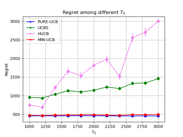
We perform numerical experiments to evaluate MIN-UCB. We compare MIN-UCB with three related benchmarks. The first policy is vanilla UCB (Auer et al., 2002) that ignores the offline data, which we call “PURE-UCB”. The second policy chooses an arm with the largest defined in (6), which we call “UCBS”. The third policy is HUCB1 (Shivaswamy & Joachims, 2012), which we call ”HUCB”.
In all experiments, we simulate our algorithm MIN-UCB and benchmarks on several instances, with fixed . Each arms’s offline and online reward follows standard Gaussian distribution with mean , , respectively. In each specific instance, we run each algorithms 100 times and report their average and standard error. For simplicity, we assume for any sub-optimal arm and for any arm . The detailed setup is provided in Appendix D.
Figure 1(a) plots the regret on single instance under different valid bias bounds , with in each trial. Specifically, for , we illustrate the regret across different in Figures 1(b), 1(c). These results demonstrate the benefit of our algorithm. When is small, indicating that DM has a precise estimation on , our MIN-UCB and UCBS that effectively leverage the information from and offline dataset perform well. In contrary, when is large, implying a loose estimation of , the offline dataset becomes challenging to utilize effectively. In such cases, MIN-UCB’s performance aligns with PURE-UCB, and remains unaffected by looseness of that misleads the DM to believe to be much larger than the actual gap. The stable performance of MIN-UCB is in contrast with the performance of UCBS and HUCB. Thus, the robustness of our algorithm is validated through these numerical results.
Figures 2(a) and 2(b) show the regret on different , where in the first group (small ) and the second group (large ). Both figures demonstrate our MIN-UCB consistently outperforms alternative methods, irrespective of and . A noteworthy observation is that is that when the offline data is easy to leverage (small ), a larger offline dataset (increased ) results in larger improvement of our algorithm over vanilla UCB. This observation aligns with intuition, as a larger coupled with a smaller indicates more informative insights into the online distribution. Conversely, when is large and offline data is hard to utilize, increasing the size of the offline dataset () does not significantly impact the performance of MIN-UCB. This is because our algorithm can adapt to this environment and consistently align with vanilla UCB, thereby mitigating the influence of the offline data on performance.
6 Conclusion
We explore a multi-armed bandit problem with additional offline data. Our approach on how to adapt to the possibly biased offline data is novel in the literature, leading to tight and optimal regret bounds. There are some interesting future directions. For example, we can further investigate how to apply it in other online learning models, such as linear bandits and online Markov decision processes. It is also intriguing to study how other forms of metrics that can measure the distribution drift can affect and facilitate the algorithm design.
Impact Statements
This paper presents work whose goal is to advance the field of Online Learning. We primarily focus on theoretical research. There are many potential societal consequences of our work, none which we feel must be specifically highlighted here.
References
- Agarwal et al. (2017) Agarwal, A., Luo, H., Neyshabur, B., and Schapire, R. E. Corralling a band of bandit algorithms. In Kale, S. and Shamir, O. (eds.), Proceedings of the 30th Conference on Learning Theory, COLT 2017, Amsterdam, The Netherlands, 7-10 July 2017, volume 65 of Proceedings of Machine Learning Research, pp. 12–38. PMLR, 2017.
- Auer et al. (2002) Auer, P., Cesa-Bianchi, N., and Fischer, P. Finite-time analysis of the multiarmed bandit problem. Mach. Learn., 47(2–3):235–256, may 2002. ISSN 0885-6125. URL https://doi.org/10.1023/A:1013689704352.
- Banerjee et al. (2022) Banerjee, S., Sinclair, S. R., Tambe, M., Xu, L., and Yu, C. L. Artificial replay: a meta-algorithm for harnessing historical data in bandits. arXiv preprint arXiv:2210.00025, 2022.
- Ben-David et al. (2010) Ben-David, S., Blitzer, J., Crammer, K., Kulesza, A., Pereira, F., and Vaughan, J. W. A theory of learning from different domains. Mach. Learn., 79(1–2):151–175, may 2010. ISSN 0885-6125.
- Besbes et al. (2022) Besbes, O., Ma, W., and Mouchtaki, O. Beyond iid: data-driven decision-making in heterogeneous environments. In Koyejo, S., Mohamed, S., Agarwal, A., Belgrave, D., Cho, K., and Oh, A. (eds.), Advances in Neural Information Processing Systems, volume 35, pp. 23979–23991. Curran Associates, Inc., 2022.
- Blanchet et al. (2019) Blanchet, J., Kang, Y., and Murthy, K. Robust wasserstein profile inference and applications to machine learning. Journal of Applied Probability, 56(3):830–857, 2019.
- Bouneffouf et al. (2019) Bouneffouf, D., Parthasarathy, S., Samulowitz, H., and Wistuba, M. Optimal exploitation of clustering and history information in multi-armed bandit. In Proceedings of the 28th International Joint Conference on Artificial Intelligence, pp. 2016–2022, 2019.
- Bu et al. (2020) Bu, J., Simchi-Levi, D., and Xu, Y. Online pricing with offline data: Phase transition and inverse square law. In International Conference on Machine Learning, pp. 1202–1210. PMLR, 2020.
- Chen et al. (2022) Chen, X., Shi, P., and Pu, S. Data-pooling reinforcement learning for personalized healthcare intervention. arXiv preprint arXiv:2211.08998, 2022.
- Crammer et al. (2008) Crammer, K., Kearns, M., and Wortman, J. Learning from multiple sources. Journal of Machine Learning Research, 9(57):1757–1774, 2008. URL http://jmlr.org/papers/v9/crammer08a.html.
- Cutkosky et al. (2021) Cutkosky, A., Dann, C., Das, A., Gentile, C., Pacchiano, A., and Purohit, M. Dynamic balancing for model selection in bandits and rl. In International Conference on Machine Learning, pp. 2276–2285. PMLR, 2021.
- Cutkosky et al. (2022) Cutkosky, A., Dann, C., Das, A., and Zhang, Q. Leveraging initial hints for free in stochastic linear bandits. In Dasgupta, S. and Haghtalab, N. (eds.), Proceedings of The 33rd International Conference on Algorithmic Learning Theory, volume 167 of Proceedings of Machine Learning Research, pp. 282–318. PMLR, 29 Mar–01 Apr 2022.
- Gur & Momeni (2022) Gur, Y. and Momeni, A. Adaptive sequential experiments with unknown information arrival processes. Manufacturing & Service Operations Management, 24(5):2666–2684, 2022.
- Hao et al. (2023) Hao, B., Jain, R., Lattimore, T., Van Roy, B., and Wen, Z. Leveraging demonstrations to improve online learning: Quality matters. In Proceedings of the 40th International Conference on Machine Learning, ICML’23. JMLR.org, 2023.
- Lattimore & Szepesvári (2020) Lattimore, T. and Szepesvári, C. Bandit algorithms. Cambridge University Press, 2020.
- Lee et al. (2021) Lee, J., Pacchiano, A., Muthukumar, V., Kong, W., and Brunskill, E. Online model selection for reinforcement learning with function approximation. In International Conference on Artificial Intelligence and Statistics, pp. 3340–3348. PMLR, 2021.
- Liu & Li (2016) Liu, C.-Y. and Li, L. On the prior sensitivity of thompson sampling. In Ortner, R., Simon, H. U., and Zilles, S. (eds.), Algorithmic Learning Theory, pp. 321–336, Cham, 2016. Springer International Publishing.
- Mansour et al. (2009) Mansour, Y., Mohri, M., and Rostamizadeh, A. Domain adaptation: Learning bounds and algorithms. arXiv preprint arXiv:0902.3430, 2009.
- Pacchiano et al. (2020) Pacchiano, A., Phan, M., Abbasi Yadkori, Y., Rao, A., Zimmert, J., Lattimore, T., and Szepesvari, C. Model selection in contextual stochastic bandit problems. Advances in Neural Information Processing Systems, 33:10328–10337, 2020.
- Pacchiano et al. (2023) Pacchiano, A., Dann, C., and Gentile, C. Data-driven regret balancing for online model selection in bandits. CoRR, abs/2306.02869, 2023. URL https://doi.org/10.48550/arXiv.2306.02869.
- Rakhlin & Sridharan (2013a) Rakhlin, A. and Sridharan, K. Online learning with predictable sequences. In Conference on Learning Theory, pp. 993–1019. PMLR, 2013a.
- Rakhlin & Sridharan (2013b) Rakhlin, S. and Sridharan, K. Optimization, learning, and games with predictable sequences. Advances in Neural Information Processing Systems, 26, 2013b.
- Russo & Roy (2016) Russo, D. and Roy, B. V. An information-theoretic analysis of thompson sampling. Journal of Machine Learning Research, 17(68):1–30, 2016. URL http://jmlr.org/papers/v17/14-087.html.
- Russo & Van Roy (2014) Russo, D. and Van Roy, B. Learning to optimize via information-directed sampling. Advances in Neural Information Processing Systems, 27, 2014.
- Shivaswamy & Joachims (2012) Shivaswamy, P. and Joachims, T. Multi-armed bandit problems with history. In Artificial Intelligence and Statistics, pp. 1046–1054. PMLR, 2012.
- Si et al. (2023) Si, N., Zhang, F., Zhou, Z., and Blanchet, J. Distributionally robust batch contextual bandits. Management Science, 69(10):5772–5793, 2023.
- Simchowitz et al. (2021) Simchowitz, M., Tosh, C., Krishnamurthy, A., Hsu, D. J., Lykouris, T., Dudik, M., and Schapire, R. E. Bayesian decision-making under misspecified priors with applications to meta-learning. In Ranzato, M., Beygelzimer, A., Dauphin, Y., Liang, P., and Vaughan, J. W. (eds.), Advances in Neural Information Processing Systems, volume 34, pp. 26382–26394. Curran Associates, Inc., 2021.
- Steinhardt & Liang (2014) Steinhardt, J. and Liang, P. Adaptivity and optimism: An improved exponentiated gradient algorithm. In International conference on machine learning, pp. 1593–1601. PMLR, 2014.
- Tennenholtz et al. (2021) Tennenholtz, G., Shalit, U., Mannor, S., and Efroni, Y. Bandits with partially observable confounded data. In Uncertainty in Artificial Intelligence, pp. 430–439. PMLR, 2021.
- Wagenmaker & Pacchiano (2023) Wagenmaker, A. and Pacchiano, A. Leveraging offline data in online reinforcement learning. In Proceedings of the 40th International Conference on Machine Learning, ICML’23. JMLR.org, 2023.
- Wang et al. (2021) Wang, Z., Zhang, C., Singh, M. K., Riek, L. D., and Chaudhuri, K. Multitask bandit learning through heterogeneous feedback aggregation. In Banerjee, A. and Fukumizu, K. (eds.), The 24th International Conference on Artificial Intelligence and Statistics, AISTATS 2021, April 13-15, 2021, Virtual Event, volume 130 of Proceedings of Machine Learning Research, pp. 1531–1539. PMLR, 2021.
- Wei & Luo (2018) Wei, C. and Luo, H. More adaptive algorithms for adversarial bandits. In Bubeck, S., Perchet, V., and Rigollet, P. (eds.), Conference On Learning Theory, COLT 2018, Stockholm, Sweden, 6-9 July 2018, volume 75 of Proceedings of Machine Learning Research, pp. 1263–1291. PMLR, 2018.
- Wei et al. (2020a) Wei, C.-Y., Luo, H., and Agarwal, A. Taking a hint: How to leverage loss predictors in contextual bandits? In Abernethy, J. and Agarwal, S. (eds.), Proceedings of Thirty Third Conference on Learning Theory, volume 125 of Proceedings of Machine Learning Research, pp. 3583–3634. PMLR, 09–12 Jul 2020a.
- Wei et al. (2020b) Wei, C.-Y., Luo, H., and Agarwal, A. Taking a hint: How to leverage loss predictors in contextual bandits? In Conference on Learning Theory, pp. 3583–3634. PMLR, 2020b.
- Ye et al. (2020) Ye, L., Lin, Y., Xie, H., and Lui, J. Combining offline causal inference and online bandit learning for data driven decision. arXiv preprint arXiv:2001.05699, 2020.
- Zhang et al. (2019) Zhang, C., Agarwal, A., Iii, H. D., Langford, J., and Negahban, S. Warm-starting contextual bandits: Robustly combining supervised and bandit feedback. In International Conference on Machine Learning, pp. 7335–7344. PMLR, 2019.
Appendix A More Detailed Comparisons with Existing Works
A.1 Comparing with (Zhang et al., 2019)
(Zhang et al., 2019) consider a stochastic contextual -armed bandit model with possibly biased offline data, which generalizes our setting of stochastic -armed bandits. On one hand, their proposed algorithm ARROW-CB does not require any knowledge on the discrepancy between the offline and online data, while our proposed algorithm requires knowing an upper bound to for each . On the other hand, in the case of stochastic -armed bandits, the regret bound of ARROW-CB (see Theorem 1 in (Zhang et al., 2019)) is at least the regret bound of the explore-then-commit algorithm (see Chapter 6 in (Lattimore & Szepesvári, 2020)) that ignores all offline data, which in particular does not offer improved regret bound compared to existing baselines that do not utilize offline data.
In more details, the ARROW-CB algorithm inputs an exploration probability parameter , and a set of weighted combination parameters that hedges between ignoring all offline data and incorporating all offline data. In their contextual setting where they compare ARROW-CB with a benchmark policy class , they establish the following regret upper bound on ARROW-CB on an instance :
| (17) |
The function (see Equation (4) in (Zhang et al., 2019)) is a discrepancy measure on the distance between the offline and online models, with the property that for all .
On one hand, (17) provides improvements to the conventional regret bound in terms of the dependency on when is sufficiently small. On the other hand, the (17) does not provide any improvement to the conventional regret bounds in the stochastic -armed bandits setting. Indeed, in -armed setting we have , where consists of the policies of always pulling arm , for . Ignoring the non-negative term and optimizing in the remaining terms show that the remaining terms sum to at least
which is no better than the explore-then-commit policy’s regret of .
Finally, one additional distinction is that (Zhang et al., 2019) requires , while we allow the offline sample sizes to be arbitrary non-negative integers.
A.2 Comparing wtih Online Learning with Advice
The frameworks of (Rakhlin & Sridharan, 2013a; Steinhardt & Liang, 2014; Wei & Luo, 2018; Wei et al., 2020a) utilize a commonly defined quantity to quantify the error in the predictions, which are provided in an online manner. We focus our discussion on comparison with (Wei & Luo, 2018). The framework of (Wei & Luo, 2018) provides the following results for adversarial multi-armed bandits with side information. Consider a -armed bandit model, where an arm is associated with loss at time for , and the loss vectors over the horizon of time steps are generated by an oblivious adversary. Before choosing an arm at time , the agent is endowed with a prediction , where is a prediction on . They design a version of optimistic online mirror design algorithm that incoporates the predictions , and achieves an expected regret bound of
| (18) |
where the expectation is taken over the internalized randomization of the algorithm, where an arm is randomly chosen each round. The quantity represents the prediction errors.
We argue that their framework can only guarantees a in terms of expected regret bound in our setting, since the prediction error term depends on the realized losses rather than their means. Indeed, In our stochastic setting (translated to a loss minimization instead of reward maximization model), the loss vectors are are independent and identically distributed according to a common (but latent) distribution . Consider the case when the loss of arm is distributed according to the Bernoulli distribution with mean for each . Even in the case when we have the prediction for each , namely the predictions reveal the true mean, we still have for each arm with certainty, leading to .
The framework of (Wei & Luo, 2018) can only gauranttee a regret bound of when . In our setting, it requires that , meaning that the prediction has to be correlated with, thus contains information of, the realized loss , for many time rounds . Different from (Wei & Luo, 2018), we achieve a regret bound of in the presense of accurate offline data, instead of receiving hints about the realized online rewards. A similar conclusion (with a worse regret bound than (18)) holds when we compare our results with (Wei et al., 2020a), which presents regret bounds on adversarial contextual bandits with predictions, since their regret bounds are also defined in terms of mentioned above.
A.3 Comparing with (Chen et al., 2022)
(Chen et al., 2022) explores a Finite-Horizon Reinforcement Learning Model incorporating possibly biased historical data, another generalization of our stochastic multi-armed bandit model. Similar to our work, their approach ”Data-pooling Perturbed LSVI” (Algorithm 2) requires an upper bound on the discrepancy between offline and online data, defined as in their Assumption 1. They propose an cross-validation method and illustrate through a case study that a substantial range of values produce similar performance for their algorithm. However, their approach cannot facilitate the design of an algorithm that achieve our improved regret bounds compared to existing benchmarks that neglects the offline data.
In details, their “Data-pooling Perturbed LSVI” algorithm is based on classical Value Iteration (VI). They adapt the VI on online learning setting by randomly perturbing the estimated value-go-functions, and applying least squares fitting to estimate the Q-function. This approach is fundemantally different from the OFU principle we apply in the multi-armed bandit context. Besides, they follow a different way to combine offline and online data. Specifically, they compute a weighted parameter that balances between online and offline data, via , , and , where refers to the number of offline samples for pair , refering to epoch , state , and action , respectively. This is shown in their equation (10). They derive the following regret upper bound:
| (19) |
where , , are their input parameter, is the length of a horizon, and is the number of state. , , are confidence radius defined in their Appendix EC.4.2. They state that when and is small (See their Theorem EC.1), this regret bound is strictly smaller than the case that without combining historical data.
However, (19) does not offer an explicit closed-form bound, and they do not provide any regret lower bound.More importantly, their implicit bound solely depends on , which is equivalent to in our model. In contrast, both our instance dependent bound (Theorem 4.2) and instance independent bound (Theorem 4.9) demonstrate how the difference in among different arms affects the regret. Thus, their approach cannot deliver the tight regret bounds on and insights into our model.
Appendix B Proofs for Regret Upper Bounds
B.1 Proof for Lemma 4.1
The proof uses the Chernoff inequality:
Proposition B.1 (Chernoff Inequality).
Let be independent (though not necessarily identically distributed) 1-subGaussian random variables. For any , it holds that
Proof of Lemma 4.1.
To prove the Lemma, it suffices to prove that . Indeed, the inequality implies by setting , and then a union bound on the failure probabilities of for establishes the Lemma. Now, we have
| (20) | ||||
| (21) | ||||
| (22) |
Step (20) is by the input assumption that . Step (21) is by a union bound over all possible values of . Step (22) is by the Chernoff inequality.
Next,
| (23) | ||||
| (24) |
The justifications of (23, 24) are the same as (21, 22) respectively. Altogether, the Lemma is proved.
∎
B.2 Proof of instance dependent regret upper bound
B.2.1 Proof of Lemma 4.8
We consider two main cases depending on and :
Case 1: . The case condition implies that
To proceed. we consider two sub-cases:
Sub-case 1a: . Then
| (25) |
The second inequality is by the lower bound in the case condition in Sub-case 1a. In addition,
Consequently, conditioned on event ,
| (26) | ||||
| (27) |
The strict inequality in step (27) is by the sub-case condition that . The less-than-equal steps in Lines (26, 27) is by conditioning on the event . Altogether, with certainty.
Sub-case 1b: . In this case, we clearly have
Consequently, we have
leading to
thus with certainty.
Case 2: . Then , and . Similar to Case 1b, we arrive at
Consequently,
where the first and the last inequalities are by the event . Altogether, with certainty.
Altogether, all cases are covered and the Lemma is proved.
B.2.2 Proof of Theorem 4.2
Applying Lemma 4.8, we get
and
and . Altogether, we arrive at
| (28) |
where , which proves the Theorem.
B.3 Proof for instance independent regret upper bounds
B.3.1 Proof of Theorem 4.9
Conditioned on , we have
| Reg | ||||
| (29) | ||||
| (30) |
Step (29) is by applying Lemma 4.1, and noting that in the upper bound of in the Lemma.
The conventional analysis shows that . We next focus on upper bounding
We claim that
| (31) |
We show (31) by establishing two major claims:
Claim 1: Suppose that is an optimal solution to the following maximization problem
| s.t. | , | ||||
Then it must be the case that for all , where we recall that is the optimum of (LP).
Claim 2: . For an optimal solution to (LP), it holds that
| (32) |
We see that Claim 1 is immediately useful for proving (31), since then
where the first inequality is by the optimality of to (IP), and the fact that any realized must be feasible to (IP). The second inequality is a direct consequence of Claim 1. Claim 2 is an axuiliary claim for proving Claim 1. We postpone the proofs of these two claims to the end of the proof of the Theorem.
Given (31), for each we then have
| (33) |
Applying the feasibility of to (LP), we have
Combining the above with (33) gives
hence . Altogether, the Theorem is proved after we provide the proofs to Claims 1, 2:
Proving Claim 1 We establish the claim by a contradiction argument. Suppose there exists an arm such that . Firstly, we assert that there must exist another arm such that . If not, we then have and for all , but then
violating the constraint . Note that the equality is by Claim 2. Thus, the claimed arm exists. To this end, the condition implies that , since otherwise , which violates the non-negativity constraint on . Altogether we have established the existence of two distinct arms such that
To establish the contradiction argument, consider another solution to the displayed optimization problem in the claim, where
By the property that , , and is a feasible solution. But then we have
| (34) |
which contradicts the assumed optimality of . Thus Claim 1 is shown.
Proving Claim 2 . Now, since is feasible to the (LP), the constraints in the (LP) give us that . We establish our asserted equality by a contradition argument. Suppose there is an arm such that . Then it can be verified that the solution defined as , for all and is also a feasible solution to (LP). But then , which contradicts with the optimality of . Thus (32) is shown.
Appendix C Proofs for Regret Lower Bounds
C.1 Notational Set Up and Auxiliary Results
Notational Set Up. Consider a non-anticipatory policy and an instance with reward distribution . We denote as the joint probability distribution function on , the concatenation of the offline dataset and the online trajectory under policy on instance . For a -measurable event , we denote as the probability of holds under . For a -measurable random variable , we denote as the expectation of under the joint probability distribution function . In our analysis, we make use of being or for an arm . To lighten our notational burden, we abbreviate as .
Auxiliary Results To establish the regret lower bounds and the impossibility result, we need three auxiliary results, namely Claim 1 and Theorems C.1, C.2. Claim 1 is on the KL-divergence between Gaussian random variables:
Claim 1.
For , where , we have .
The following, dubbed Bretagnolle–Huber inequality, is extracted from Theorem 14.2 from (Lattimore & Szepesvári, 2020):
Theorem C.1.
Let be probability disributions on . For an event , it holds that
Lastly, the derivation of the chain rule in Theorem C.2 largely follows from the derivation of Lemma 15.1 in (Lattimore & Szepesvári, 2020):
Theorem C.2.
Consider two instances that share the same arm set , online phase horizon , offline sample size , but have two different reward distributions , . For any non-anticipatory policy , it holds that
We provide a proof to theorem C.2 for completeness sake:
Proof of Theorem C.2.
The proof largely follow the well-known chain rule in the multi-armed bandit literature, for example see Lemma 15.1 in (Lattimore & Szepesvári, 2020). We start by explicitly expressing the joint probability function on
under reward distribution and non-anticipatory policy . In coherence with our focus on Gaussian instances, we only consider the case when all the random rewards (offline or online) are continuous random variables with support on . Generalizing the argument to general reward distributions only require notational changes. By an abuse in notation, we denote as the probability density function (with variable ) of the offline reward distribution with arm , and likewise for the online reward distribution.
To ease the notation, we denote . Then is expressed as
| (35) |
Likewise, by replacing reward distribution with but keeping the fixed policy unchanged, we have
The KL divergence between and is
where , and .
We use the explicit expressions of to decompose the log term:
In the second line, the middle sum is equal to zero, which can be interpreted as the fact that we are evaluating the same policy on reward distributions . Finally, marginalizing and making use of (35) gives, for each ,
| (36) |
where the first equality in (36) follows by integrating with respect to over and then summing over in the order of , and then integrating over all variables in except . For each during the online phase we have
| (37) |
Summing (36) over and , as well as summing (37) over establish the Theorem. ∎
C.2 Proof for Proposition 3.1, the Impossibility Result
By the condition , we know that , so in the instance with , arm 2 is the unqiue optimal arm. Consider the event . Now,
| (38) | ||||
| (39) |
Step (38) is again by the chain rule in Theorem C.2. Step (39) is because . It is evident that
and by the Claim assumption that , we have
which leads to
Again by the Proposition assumption , we arrive at the claimed inequality, and the Proposition is proved.
C.3 Proof for instance dependent regret lower bound
C.3.1 Proof for Theorem 4.7
We denote as the means of the Gaussian distributions respestively, for each arm . In addition, recall the notation that , and .
Consider an arbitrary but fixed arm with . We claim that
| (40) |
The Lemma then follows by applying (40) on each sub-optimal arm, thus it remains to prove (40). To proceed, we consider another Gaussain instance , where
but
| (41) |
It is clear that implies . Indeed, if the second case in (41) holds, then the mean of the mean of is equal to , while if the first case hold, then we evidently have
thus . Consider the event . By the assumed consistency of , we have
| (42) | ||||
| (43) | ||||
| (44) |
Step (42) is by the definition of consistency. Step (43) is implied by our construction that in instance , arm is sub-optimal with optiamlity gap , and in instance , arm is the unique optimal arm and other arms have optimality gap at least . Step (44) is by the Chain rule Theorem C.2, as well as the BH inequality. By our set up, we have
Plugging in we get
| (45) |
which is equivalent to
Rearranging leads to the claimed inequality (40), and the Lemma is proved.
C.4 Proof for instance independent regret lower bound
C.4.1 Proof for Theorem 4.10
We proceed by a case analysis:
Case 1a: , and . We derive a regret lower bound of
Case 1b: , and . We derive a regret lower bound of
Case 2: . We derive a regret lower bound of
We establish the three cases in what follows.
Case 1a: , and . We derive a regret lower bound of
Now, without loss of generality, we assume that . Consider the following Gaussian reward distributions with (thus for any ), defined as
Consider the values defined as for each , and . Evidently, is feasible to (LP), and thus we have , the optimum of (LP). In particular, there exists an arm such that . To this end, let’s consider two situations:
Situation (i): for all . The condition immeidately implies . Then we can deduce that for all , which further implies that for all since . The above implies that , which implies that
Situation (ii): for a . In this case, consider the following Gaussian reward distribution with , defined as
To this end, note that for all , but . In addition, both belong to . Consider the event . We have
| (46) | ||||
| (47) | ||||
| (48) |
Altogether, in Case 1a, we either have
or
Case 1b: , and . We derive a regret lower bound of
Now, set , and consider the Guassian instance with reward disribution :
Now, there exists an arm such that . Consider the Gaussian instance with
To this end, note that for all , and for all , but . In addition, both belong to . Consider the event . We have
| (49) | ||||
| (50) | ||||
| (51) |
Step (49) is again by Theorem C.1. Step (50) is by the Chain rule (Theorem C.2), and our observations on the constructed . Step (54) is by the choice of arm and the KL divergence between . The strict inequality in (51) is by the case assumption that , which implies . The larger than equal in (51) is by the assumption that . Altogether, the desire regret lower bound of
is achieved.
Case 2: . We derive a regret lower bound of
largely by following Case 1b with a different , as well as the proof of Lemma 15.2 in (Lattimore & Szepesvári, 2020). Recall since , so the case condition implies , meaning . Now, set , and consider the Guassian instance with reward disribution :
Now, there exists an arm such that . Consider the Gaussian instance with
To this end, note that for all , and for all , but . In addition, both belong to . Consider the event . We have
| (52) | ||||
| (53) | ||||
| (54) |
Step (52) is again by Theorem C.1. Step (53) is by the Chain rule (Theorem C.2), and our observations on the constructed . Step (54) is by the choice of arm and the KL divergence between . Finally, putting in gives us
Altogether, the three cases cover all possibilites and the Theorem is proved.
Appendix D More Details on Numerical Experiments
In all experiments, we set (hence ). In Figure 1, we set , , and vary from 0.1 to 0.6. In Figure 2, we set , , and vary from 1000 to 3000, for , respectively.