[table]capposition=top
Lesion Search with Self-supervised Learning
Abstract
Content-based image retrieval (CBIR) with self-supervised learning (SSL) accelerates clinicians’ interpretation of similar images without manual annotations. We develop a CBIR from the contrastive learning SimCLR and incorporate a generalized-mean (GeM) pooling followed by L2 normalization to classify lesion types and retrieve similar images before clinicians’ analysis. Results have shown improved performance. We additionally build an open-source application for image analysis and retrieval. The application is easy to integrate, relieving manual efforts and suggesting the potential to support clinicians’ everyday activities.
1 Introduction
Radiologists’ interpretation of lesions (nodules, tumor-like, and surface-like) requires careful analysis. Lesion images employ a wide variety of sizes, shapes (e.g., elliptical, irregular), colors (e.g., grayscale), and textures (e.g., convex, nodule, distortion) (Hofman & Hicks (2016)), which makes manual image retrieval or content-based image retrieval (CBIR) with annotations time-consuming and at risk of errors. Annotating lesions is expensive because of intra-class variations: the same lesion type may not be visually similar, while different lesion types may appear similarly once images are taken at similar stages of disease progression. In this work, we first develop the SSL method for lesion feature extraction that is prepared for image retrieval and classification tasks. The overall pipeline is shown in Figure 1. Second, we developed a web-based open-source DICOM (Digital Imaging and Communications in Medicine) application for Radiology image analysis and similar lesion image retrieval, shown in Figure 2. Easy Python installation can be found at https://github.com/openhcimed/flask_search.

2 Application: DICOM User Interface
The application comprises two components: UI front-end and CBIR back-end. UI front-end is an AngularJS-based viewer with toolbars. Users can drag and drop single or batch images for analysis, such as adjusting timeframes, zooming, color contrast, annotations, and viewing metadata. Annotations are in JSON format and can be saved locally or sent to the CBIR back-end SSL model.

Back-end model. First, we preprocessed regions of interest and applied the Hessian-based Frangi filter (Frangi et al. (1998); Kroon & Schrijver (2009); Longo et al. (2020)) to maximize lesions while minimizing noise. Details are in Appendix A. Second, the baseline started with a robust SimCLR (Chen et al. (2020)) with ResNet-18 (He et al. (2016)). To improve image retrieval, we used a generalized-mean (GeM) pooling layer (Radenović et al. (2018)) followed by L2 normalization. We trained networks on the public DeepLesion dataset (Yan et al. (2018)) without patients’ identifications, reliving data privacy concerns. Data details are in Appendix B. Finally, CBIR ranked candidate descriptors in ascending order according to their closest cosine distances to a query . We chose top-9 candidates to cover enough similarity. Furthermore, experimental details are in Appendix C. Loss function and distance details are in Appendix D.
3 Results
Classification results. We started comparisons between two baselines: SimCLR and VAE (Variational AutoEncoder), utilizing ResNet-18. Table 1 shows that either applying the Frangi filter during preprocessing or GeM pooling layer with L2-normalization results in improvements from baselines, but to a different extent. Frangi filter provides a much stronger improvement over SimCLR, yet combining it with the GeM approach results in the most effective feature extractor. However, using Frangi filter has limitations, as varying parameters may produce discrepancies within the dataset or in a different dataset. We observed benefits from these combinations, but it’s apparent that these methods are off-the-shelf and are not compared with novel SSL networks. Furthermore, the performance on other medical datasets to solve more problems is unknown, which is left for future work.
| Base model | Frangi | +GeM | Accuracy (%) | F1-score (%) |
|---|---|---|---|---|
| SimCLR | 64.52 | 65.57 | ||
| SimCLR | 80.39 | 78.93 | ||
| SimCLR | 69.24 | 67.74 | ||
| SimCLR | 80.73 | 77.83 | ||
| VAE | 74.04 | 68.83 | ||
| VAE | 74.35 | 75.79 | ||
| VAE | 76.34 | 73.78 | ||
| VAE | 76.04 | 75.24 |
CBIR results. As shown in Appendix E Table 2, we assess the same patient (intra-patient), across different patients (inter-patient), and all patients, as per commonly used clinical evaluations. The standard retrieval metrics, mAP@10 and Precision@k, suggest that intra-patient retrieval precision is higher because of highly similar features within a single patient, while features are dissimilar between different patients. Furthermore, results indicate that the SimCLR model (contrastive-based) outperforms the VAE model (generative-based).
4 Conclusions
We present an open-source interactive application that facilitates lesion analysis and retrieval based on self-supervised learning (SSL). Developed from the contrastive learning SimCLR, with Frangi filter, GeM pooling and L2-normalization together improve lesion retrieval performance.
URM Statement
The authors acknowledge that at least one key author of this work meets the URM criteria of ICLR 2023 Tiny Papers Track.
References
- Chen et al. (2020) Ting Chen, Simon Kornblith, Mohammad Norouzi, and Geoffrey Hinton. A simple framework for contrastive learning of visual representations. In International conference on machine learning, pp. 1597–1607. PMLR, 2020.
- Frangi et al. (1998) Alejandro F Frangi, Wiro J Niessen, Koen L Vincken, and Max A Viergever. Multiscale vessel enhancement filtering. In International conference on medical image computing and computer-assisted intervention, pp. 130–137. Springer, 1998.
- Gómez (2019) R Gómez. Understanding ranking loss, contrastive loss, margin loss, triplet loss, hinge loss and all those confusing names. Raúl Gómez blog, pp. 12, 2019.
- He et al. (2016) Kaiming He, Xiangyu Zhang, Shaoqing Ren, and Jian Sun. Deep residual learning for image recognition. In Proceedings of the IEEE conference on computer vision and pattern recognition, pp. 770–778, 2016.
- Hofman & Hicks (2016) Michael S Hofman and Rodney J Hicks. How we read oncologic fdg pet/ct. Cancer Imaging, 16(1):1–14, 2016.
- Krizhevsky et al. (2012) Alex Krizhevsky, Ilya Sutskever, and Geoffrey E Hinton. Imagenet classification with deep convolutional neural networks. Advances in neural information processing systems, 25:1097–1105, 2012.
- Kroon & Schrijver (2009) Dirk-Jan Kroon and M Schrijver. Hessian based frangi vesselness filter. MATLAB File Exchange, 24409, 2009.
- Longo et al. (2020) Antonia Longo, Stefan Morscher, Jaber Malekzadeh Najafababdi, Dominik Jüstel, Christian Zakian, and Vasilis Ntziachristos. Assessment of hessian-based frangi vesselness filter in optoacoustic imaging. Photoacoustics, 20:100200, 2020.
- Pham et al. (2018) Tri-Cong Pham, Chi-Mai Luong, Muriel Visani, and Van-Dung Hoang. Deep cnn and data augmentation for skin lesion classification. In Asian Conference on Intelligent Information and Database Systems, pp. 573–582. Springer, 2018.
- Radenović et al. (2018) Filip Radenović, Giorgos Tolias, and Ondřej Chum. Fine-tuning cnn image retrieval with no human annotation. IEEE transactions on pattern analysis and machine intelligence, 41(7):1655–1668, 2018.
- Tariq et al. (2021) Mehreen Tariq, Sajid Iqbal, Hareem Ayesha, Ishaq Abbas, Khawaja Tehseen Ahmad, and Muhammad Farooq Khan Niazi. Medical image based breast cancer diagnosis: State of the art and future directions. Expert Systems with Applications, 167:114095, 2021.
- van Tulder & de Bruijne (2016) Gijs van Tulder and Marleen de Bruijne. Combining generative and discriminative representation learning for lung ct analysis with convolutional restricted boltzmann machines. IEEE transactions on medical imaging, 35(5):1262–1272, 2016.
- Yan et al. (2018) Ke Yan, Xiaosong Wang, Le Lu, and Ronald M Summers. Deeplesion: automated mining of large-scale lesion annotations and universal lesion detection with deep learning. Journal of medical imaging, 5(3):036501, 2018.
- You et al. (2017) Yang You, Igor Gitman, and Boris Ginsburg. Large batch training of convolutional networks. arXiv preprint arXiv:1708.03888, 2017.
Appendix
Appendix A Frangi Filter for Lesion Detection
Frangi filter function has two components and represents eigenvalues (Frangi et al. (1998)): if either or , . Otherwise:
| (1) |
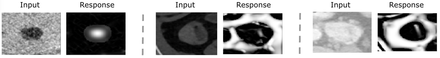
where , , and . The modification enhances contours by restricting such that at the scale “s”. To suppress background noises that are not contours, we set = 0 if , and change and into high eigenvalues to control close to 1, which differentiates blob-like and plate-like lesion structures from others. Threshold parameters are , , and to balance sensitivity differentiating blob-like and plate-like lesions from background noises. To capture lesions with various sizes, we modify the multiscale value, ”s”, from 1 to 9 with a step size of . A few examples comparing original ROIs and responses after applying the new function are shown in Figure 3.
Appendix B Dataset
DeepLesion Dataset. Previously, most algorithms considered one or a few types of lesions (Pham et al. (2018); Tariq et al. (2021); van Tulder & de Bruijne (2016)). Yan et al. developed the large and publicly available DeepLesion dataset from the NIH Clinical Center (Yan et al. (2018)) towards developing universal lesion detections. In clinical practice, DeepLesion dataset is widely accepted for monitoring cancer patients due to its recorded diameters in accordance with the Solid Tumor Response Evaluation Criteria (RECIST), which is one of the commonly used means of criteria. DeepLesion dataset consists of 33,688 PACS-bookmarked CT images from 10,825 studies of 4,477 unique patients (Yan et al. (2018)). It includes various lesions across the human body, such as lungs, lymph, liver, etc. Four cardinal directions (left, top, right, bottom) enclose each lesion in every CT slice as a bounding box to mark coarse annotations with labels. We crop regions of interest (ROIs) based on these bounding boxes instructed in the dataset to comprise excessive instances for model training.
Appendix C Experimental setup
Data pre-processing.
We preprocess DeepLesion by cropping bounding boxes, flips, color distortions, and Gaussian blur. We keep the image size as 64 x 64 and apply the Frangi filter.
Implementation Details.
We train models with Pytorch (Krizhevsky et al. (2012)) on a single Nvidia DGX-A100 GPU. We implement ResNet-18 (He et al. (2016)) in SimCLR, followed by two more convolutional layers and a GeM pooling layer with L2-normalization. We performed 1000 epochs for SSL pre-training with LARS (You et al. (2017)) optimizer of a learning rate, a weight decay, and a cosine learning rate scheduler. For CBIR task, we compute contrastive loss with margin 0.8 and cosine distance from the sigmoid classification layer. Optimized with SGD, we fine-tune the model for 50 iterations with a learning rate of 0.01, momentum of 0.9, and tracker of cosine growth for the learning rate.
Appendix D CBIR Descriptors for the Most Similar Lesions.
We used the following loss function: (Gómez (2019))
| (2) |
is an anchor, is a positive sample sharing the same lesion type with . is a negative sample different from ’s type. is the margin determining the stretch for separating negative and positive samples. We use cosine distance similarity measure d to imply how similar a retrieved candidate is to a given query:
| (3) |
is a query and is a lesion candidate embedding.
Appendix E CBIR Results
| Evaluation setting | Method | mAP@10 | Precision@1 | Precision@10 |
|---|---|---|---|---|
| All-patients | VAE | 0.688 | 0.699 | 0.581 |
| SimCLR | 0.729 | 0.734 | 0.643 | |
| Same-patient | VAE | 0.707 | 0.746 | 0.630 |
| SimCLR | 0.713 | 0.757 | 0.633 | |
| Cross-patient | VAE | 0.378 | 0.408 | 0.370 |
| SimCLR | 0.465 | 0.503 | 0.458 |