LEGAN: Disentangled Manipulation of Directional Lighting and Facial Expressions whilst Leveraging Human Perceptual Judgements ††thanks: *Work done while at Affectiva
Abstract
Building facial analysis systems that generalize to extreme variations in lighting and facial expressions is a challenging problem that can potentially be alleviated using natural-looking synthetic data. Towards that, we propose LEGAN, a novel synthesis framework that leverages perceptual quality judgments for jointly manipulating lighting and expressions in face images, without requiring paired training data. LEGAN disentangles the lighting and expression subspaces and performs transformations in the feature space before upscaling to the desired output image. The fidelity of the synthetic image is further refined by integrating a perceptual quality estimation model, trained with face images rendered using multiple synthesis methods and their crowd-sourced naturalness ratings, into the LEGAN framework as an auxiliary discriminator. Using objective metrics like FID and LPIPS, LEGAN is shown to generate higher quality face images when compared with popular GAN models like StarGAN and StarGAN-v2 for lighting and expression synthesis. We also conduct a perceptual study using images synthesized by LEGAN and other GAN models and show the correlation between our quality estimation and visual fidelity. Finally, we demonstrate the effectiveness of LEGAN as training data augmenter for expression recognition and face verification tasks.
1 Introduction
Deep learning [59] has engendered tremendous progress in automated facial analysis, with applications ranging from face verification [72, 22, 11] to expression classification [92]. However, building robust and accurate models that generalize effectively in-the-wild is still an open problem. A major part of it stems from training datasets failing to represent the “true” distribution of real world data [54, 68, 93, 6] (\egextreme lighting conditions [17, 73, 38]); or the training set may be non-uniformly distributed across classes, leading to the long-tail problem [63].
One way to mitigate the imbalance problem, shown to work in multiple domains [62, 9, 15, 100], is to introduce synthetic samples into the training set. Many approaches for generating synthetic data exist [18, 8, 42], none as successful as GANs [37] in generating realistic face images [16, 51, 52, 25]. Thus, in this work, we design a GAN model for synthesizing variations of an existing face image with the desired illumination and facial expression, while keeping the subject identity and other attributes constant. These synthetic images, when used as supplemental training data, can help build facial analysis systems that better generalize across variations in illumination and expressions.


One drawback of GAN-based face generation is the absence of an accurate and automated metric to judge the perceptual quality of synthesized images [57, 20]. In order to solve this problem, we also introduce a quality estimation model that can serve as a cheap but efficient proxy for human judgment while evaluating naturalness of synthetic face images. Instead of generating a single score for a distribution of synthetic images [107, 45, 79] or for image pairs [105, 75], our goal is to infer an image-quality score on a continuum for a single synthetic face image. With this in mind, we run an Amazon Mechanical Turk (AMT) experiment where turkers are instructed to score the naturalness of synthetic face images, generated using different 3D-model [9] and GAN-based [51, 52, 78, 2] synthesis approaches. We then build a feed forward CNN to learn representations from these images that map to their corresponding perceptual rating, using a margin based regression loss.
In addition to a traditional discriminator [37], this trained quality model is then used as an auxiliary discriminator in the synthesis framework, named LEGAN (Lighting-Expression GAN), that we propose in this paper. Instead of intertwining the two tasks [25], LEGAN decomposes the lighting and expression sub-spaces using a pair of hourglass networks (encoder-decoder) that generate transformation masks capturing the intensity changes required for target generation. The desired output image is then synthesized by a third hourglass network from these two masks.
To demonstrate the effectiveness of LEGAN, we qualitatively and quantitatively compare its synthesized images with those produced by two popular GAN based models [25, 26] using objective metrics like FID [45], LPIPS [105], SSIM [95] and face match score. We also conduct a human rater study to evaluate the perceptual quality of LEGAN’s images and the contribution of the quality based auxiliary discriminator towards hallucinating perceptually superior images. Finally, we show the efficacy of LEGAN as training data augmenter by improving the generalizability of face verification and expression recognition models.
2 Related Work
Face Synthesis: Early approaches [18, 67] focused on stitching together similar looking facial patches from a gallery to synthesize a new face. Manipulating the facial shape using 3D models [49, 89, 63, 9] or deep features [27, 91] is another popular approach to generate new views. In recent times however researchers have pre-dominantly focused on using GANs [37] for synthesis, where an upsampling generator hallucinates faces from a noise vector, either randomly sampled from a distribution [37, 77, 51, 52] or interpreted from a different domain [71]. An existing face can also be encoded and then upsampled to obtain the desired attributes [48, 47, 96, 10, 70, 31, 35, 108, 23, 25].

Editing Expressions: Research in this domain started with modeling skin-muscle movements [33] for different facial expressions or swapping facial patches based on visual proximity [18]. With the advent of 3D face models, researchers used static [63] or morphable models [19, 102] to manipulate facial expressions with a higher degree of realism. Recently, the use of VAEs [13] and adversarial image-to-image translation networks have become extremely popular for editing facial expressions [48, 108, 25], with or without paired data for training. Some of these models use attention masks [76], facial shape information [36, 34] or exemplar videos [85] to guide the model in this task.
Editing Lighting: While methods like histogram equalization [74, 109] and gamma correction can shift the global luminance distribution and color encoding of an image, they cannot manipulate the direction of the light source itself. An early method [94] utilizes spherical harmonics to manipulate the directional lighting in 3D. In [24], local linear adjustments are performed on overlapping windows to change the lighting profile of an image. Deep learning based approaches have also been proposed where the reflectance, normal and lighting channels are disentangled and edited to relight images [81, 84, 83, 41]. Alternatively, the desired lighting can be passed to an encoder-decoder pair as the target for lighting manipulation in the input image [106, 86, 65, 69]. Recently, joint facial pose, lighting and expression manipulation has been proposed in [30, 58] where an input image can be manipulated by changing its attributes in feature space leveraging 3D parameters or latent information from synthetic images during training.
Quality Estimation of Synthetic Face Images: Synthetic image quality is commonly evaluated using metrics like the Inception Score [79] or FID [45], which compare statistics of real and synthetic feature distributions, and output a single score for the whole distribution rather than the individual image. The features themselves are extracted from the Inception-v3 model [87], usually pre-trained on objects from [29], and not specifically faces. As these metrics do not take into account human judgements, they do not correlate well with perceptual realism [14, 20]. Consequently, researchers run perceptual studies to score the naturalness of synthetic images [104, 8]. These ratings are also used to design models that measure distortion between real and synthetic pairs [105, 75] or the coarse realism (‘real’ vs ‘fake’) of a synthetic image [107]. None of these evaluation models however are designed specifically for face images. Recently, [57] proposed a metric to rate the perceptual quality of a single image by using binary ratings from [107] as ground truth for synthetic face images generated by [51, 52]. However, their regression based model is trained on only 4,270 images and thus insufficient to reliably model the subjective nature of human judgements.
Unlike these methods, we build a synthetic face quality estimation model by leveraging perceptual ratings of over 37,000 images generated using five different synthesis techniques [51, 52, 78, 1, 9]. Our quality model takes into account the variability in human judgements and generate a realism score for individual images rather than the whole set. We leverage this model as an auxiliary discriminator in the LEGAN framework for simultaneous lighting and facial expression manipulation. This novelty together with LEGAN’s feature disentanglement improves the naturalness of the hallucinated images. Additionally, we do not require external 3DMM information or latent vectors during training nor do we need to fine-tune our model during testing on input images [30, 58].
3 Quality Estimation Model
Our quality estimator model is trained with synthetic face images assembled and annotated in two sequential stages, as described below.
Stage I: We first generate 16,507 synthetic face images using the StyleGAN [52] generator. These images are then annotated by labelers using Amazon Mechanical Turk (AMT) on a scale of 0 - 10 for naturalness, where a 0 rating represents an unnatural image and 10 a hyper-realistic one. The images are then binned into two broad groups - ‘unnatural’ for AMT ratings between 0 - 5 and ‘natural’ for 5 - 10. We extract descriptors for each image from the ‘avg_pool’ layer of the ResNet50 [44] model, pre-trained on VGGFace2 [22] and train a linear SVM [28] with the extracted features of around 12,000 images from this dataset and use the rest for parameter tuning. Post training, we use this SVM as a rough estimator of naturalness.
Stage II: In this stage, we perform the same AMT experiment again with a larger set of synthetic face images, collected from the following datasets:
1. FaceForensics++[78] - we randomly sample 1000 frames from this dataset consisting of 1000 video sequences that have been manipulated with four automated face manipulation methods.
2. DeepFake[2, 3] - we use sampled frames from 620 manipulated videos of 43 actors from [1].
3. ProGAN [51] - we generate 10,000 synthetic face images of non-existent subjects by training NVIDIA’s progressively growing GAN model on the CelebA-HQ dataset [51].
4. StyleGAN [52] - we extract 100,000 hyper-realistic face images of non-existent subjects generated using the StyleGAN model that were pre-filtered for quality [4].
5. Notre Dame Synthetic Face Dataset [9] - we randomly sample 163,000 face images, from the available 2M, of synthetic subjects generated using ‘best-fitting’ 3D models.
To focus on near-frontal faces, we remove images with yaw over 15 in either direction, estimated using [43]. Since gender information is absent in most of the above datasets, we group the synthetic images using gender predictions from a pre-trained model [60]. Our trained SVM (from Stage I) is also used to rate the coarse naturalness of the collected images, using their ResNet50 features. We ensure balance in our synthetic dataset by sampling evenly from the natural and unnatural sets, as estimated by the SVM, and the perceived gender classes. To focus solely on the facial region, the pixels outside the convex hull formed by the facial landmarks, estimated using [21], of an image are masked. After the gender, facial yaw and naturalness based filtering, and the pre-processing step, we end up with 37,267 synthetic face images111Available here: https://github.com/Affectiva/LEGAN_Perceptual_Dataset for our second AMT experiment.
Again, we ask Turkers to rate each image for naturalness on a scale of 0 - 10. Each image is shown to a Turker for 60 seconds to allow them time to make proper judgement even with slow network connection. We divide the full set of images into 72 batches such that each batch gets separately rated by 3 different Turkers. Post crowd-sourcing, we compute the mean () and standard deviation () from the 3 scores and assign them as naturalness label for an image.
To train the quality estimation model, we use 80% of this annotated data and the rest for validation and testing. For augmentation, we only mirror the images as other techniques like translation, rotation and scaling drastically change their appearance compared to what the Turkers examined. Our model downsamples an input image using a set of strided convolution layers with Leaky ReLU [99] activation followed by two fully connected layers with linear activation and outputs a single realness scoring. Since both and are passed as image labels, we try to capture the inconsistency in the AMT ratings (i.e. the subjective nature of human perception) by formulating a margin based loss for training. The model weights are tuned such that its prediction is within an acceptable margin, set to , from the mean rating of the image. The loss can be represented as:
| (1) |
where is the batch size, is the model prediction for the -th image in the batch. Since the model is trained on the mean rating (regression) as the target rather than fixed classes (classification), pushes the model predictions towards the confidence margin from .


4 LEGAN
We build LEGAN as a lightweight network that works with unpaired data, similar to the StarGAN family, to focus more on assessing the effect of our quality estimation model () as a perceptual loss. Unlike [30, 58], LEGAN does not require additional networks to regress 3DMM parameters or fine-tuning during inference. We describe the architecture and objective functions of LEGAN in this section, an overview of which can be seen in Figure 3.
4.1 Architecture
Generator: Our generator , composed of three hourglass networks (encoder-decoder), starts with an input RGB face image and a target attributes vector that corresponds to expression and lighting conditions and respectively. The first hourglass receives concatenated with while the second one receives concatenated with , thus disentangling the transformation task. Inside each hourglass, the concatenated tensor is downsampled using strided convolutions and then passed through a set of residual blocks [44] before being upsampled using pixel shuffling layers [82]. Each convolution layer is followed by instance normalization [90] and ReLU activation [64] for non-linearity. These upsampled images are the transformation masks and that map the changes in pixel intensity required to translate to conditions specified in . and are concatenated together and fed to the third hourglass to generate the output image . The objective of dividing the generation process into two stages and hallucinating the transformation masks is two fold - (a) easing the task of each hourglass by simply making it focus on registering the required expression or lighting changes instead of both registration and hallucination, and (b) making the transformation process more explainable, with salient pixels prominent in and , as can be seen in Figure 4.
Discriminator: The discriminator takes the output image and predicts not only its realness score but also classifies its attributes . is composed of strided convolution layers with Leaky ReLU [99] activation that downsample the image to extract its encoded feature map. We use a patch discriminator [48] that takes this encoded feature map and passes it through a single channel convolution to get the realness map . This feature map is also operated by a conv layer with filters to get the attributes prediction map , where = no. of channels in .
Auxiliary Discriminator: We integrate the perceptual quality model , described in Section 3, into the LEGAN model graph to further refine the naturalness of the images synthesized by . Unlike , we do not train jointly with but use the weights of a pre-trained snapshot.
Identity Network: We also add a pre-trained identity preserving network T to estimate the deviation of the output identity from that of the input. T is trained offline on face images with different pose, expression and lighting and its weights are kept frozen throughout LEGAN’s training.
4.2 Loss Function
1. Adversarial Loss: is trained to distinguish a real face image from its synthetic counterpart and judge the realness of the hallucinated image . To stabilize the gradients and improve quality, we use the WGAN [7] based objective for this task with a gradient penalty [40], set as:
| (2) |
where is sampled uniformly from real and synthetic images and is an tunable parameter. While tries to minimize this to separate the synthetic from the real, tries to maximize it by fooling .
2. Classification Loss: To ensure the target lighting and expression are correctly rendered by and enable LEGAN to do many-to-many translations, we formulate a classification loss using ’s predictions, in the form of . The loss is computed as:
| (3) |
where and are the original and target attributes of an input image .
3. Identity Loss: To preserve the subject identity without using paired data, we add an identity loss between the input and the translated output by utilizing representations from T. Both and are passed through T for feature extraction and we set the objective to minimize the cosine distance between these two features as:
| (4) |
Ideally, the cosine distance between these two feature vectors should be 0, as they belong to the same identity.
4. Reconstruction Loss: To keep non-translating features from the input intact in the output image, we use a cyclic reconstruction loss [108] between and its reconstruction , computed as:
| (5) |
|
|
|
|
|
|
|
|||||||
|---|---|---|---|---|---|---|---|---|---|---|---|---|---|
|
38.745 | 0.126 | 0.559 | 0.635 | 5.200 | 22.3% | |||||||
|
34.045 | 0.123 | 0.567 | 0.647 | 5.391 | 34.7% | |||||||
|
54.842 | 0.212 | 0.415 | 0.202 | 5.172 | 3.75% | |||||||
|
29.964 | 0.120 | 0.649 | 0.649 | 5.853 | 39.3% | |||||||
|
12.931 | - | - | 0.739 | 5.921 | - |
|
|
|
|
|
|
||||||
|---|---|---|---|---|---|---|---|---|---|---|---|
|
43.987 | 0.302 | 0.639 | 0.622 | 6.41 | ||||||
|
41.641 | 0.268 | 0.624 | 0.614 | 6.73 | ||||||
|
59.328 | 0.445 | 0.279 | 0.213 | 6.60 | ||||||
|
38.794 | 0.271 | 0.622 | 0.628 | 6.68 | ||||||
|
- | - | - | - | 6.83 |
|
|
|
|
|
|
||||||
|---|---|---|---|---|---|---|---|---|---|---|---|
|
42.089 | 0.173 | 0.623 | 0.620 | 6.98 | ||||||
|
36.189 | 0.145 | 0.614 | 0.621 | 7.15 | ||||||
|
50.360 | 0.311 | 0.312 | 0.295 | 6.89 | ||||||
|
29.059 | 0.184 | 0.662 | 0.635 | 7.07 | ||||||
|
- | - | - | - | 7.31 |
5. Quality Loss: We use ’s predictions for further improving with perceptual realism of the synthetic images. Masked versions of the input image , the synthesized output and the reconstructed input , produced using facial landmarks extracted by [21], are used for loss computation as follows:
| (6) |
where is a hyper-parameter that can be tuned to lie between 5 (realistic) and 10 (hyper-realistic). We find synthesis results to be optimal when = 8.
Full Loss: We also apply total variation loss [50] on and to smooth boundary pixels and set the final training objective as a weighted sum of the six losses as:
| (7) |

|
|
|
|
|
|||||
|
|
0 | 0.954 0.002 | 0.966 0.002 | |||||
|
|
|
0.967 0.001 | 0.972 0.001 |
|
|
|
|
|
|
|
|||||||
|
|
0 | 0.851 0.005 | 0.955 0.001 | 0.873 0.004 | 0.887 0.005 | |||||||
|
|
|
0.868 0.005 | 0.956 0.001 | 0.890 0.003 | 0.897 0.001 |
5 Experiments and Results
Training Data. We utilize 36,657 frontal RGB images from the CMU-MultiPIE dataset [39], with 20 different lighting conditions and 6 acted facial expressions, to build our model. For training we use 33,305 images of 303 subjects and the remaining 3,352 images of 34 subjects for testing. The training data is highly skewed towards ‘Neutral’ and ‘Smile’ compared to the other 4 expressions but the distribution is almost uniform for the lighting classes. We align each image using their eye landmarks extracted with [21] and resize to 1281283. We do not fine-tune LEGAN on any other data and solely rely on its generalizability for the different experimental tasks.
Testing Data. Along with MultiPIE’s held out test set, we also utilize the AFLW [56] and CelebA [61] datasets to test the robustness of LEGAN towards in-the-wild conditions. We do not train or fine-tune LEGAN on these datasets and use the model trained on MultiPIE for translation tasks.
Augmentation: Recoloring. Since MultiPIE [39] was acquired in a controlled setting, it has more or less uniform hue and saturation across all images. To artificially inject some diversity in the overall image color, and prevent visual overfitting, we build an image colorization model. Inspired by [104], we train two separate pix2pix [48] style GAN models where the input is a grayscale image and the target is set as its colored counterpart (\ieoriginal image). To manipulate the color style of the same grayscale image differently, we train these two models with randomly sampled 10K images from the UMDFaces [12] and FFHQ [51] datasets respectively. The trained generators are used to augment the color style of the MultiPIE training set.
Augmentation: White Balancing. In addition to changing the color style, we also artificially edit the white balance of the training images by utilizing the pre-trained model from [5]. This model can automatically correct the white balance of an image or render it with different camera presets. For each training input, we randomly use it as is or select its recolored or color corrected version, and pass it to LEGAN.
Implementation Details. To learn the model, we use the Adam optimizer [55] with a learning rate of 0.0001 and parameters and set to 0.5 and 0.999 respectively. The different loss weights , , , and are set empirically to 10, 20, 10, 10, 0.5 and 0.0000001 respectively. As done in [76], we train 5 times for each training iteration of the . We train the LightCNN-29 model [98] on the CASIA-WebFace dataset [101] and utilize it as our identity network T. Features from its penultimate layer are used to compute . LEGAN is trained with a batch size of 10 on a single Tesla V100 GPU for 100 epochs.
Comparison with Other GAN Models: Our proposed model is simple and unique as it does not require 3DMM information or external synthetic images during training [30, 58] nor do we need to fine-tune our model during testing on input images. Due to this simplicity, we choose 2 popular publicly available unpaired domain translation models for comparison - StarGAN [25] and the more recent StarGAN-v2 [26]. We train these models for lighting and expression manipulation with the same MultiPIE [39] training split for 100 epochs. Additionally, to gauge the effect of on off-the-shelf models we train StarGAN separately with the auxiliary discriminator added (StarGAN w/ ).
Metrics for Quality Estimation. To evaluate the quality of synthetic face images generated by LEGAN and other GAN models, we compare the synthesized output with the corresponding target image222Since target images are not available for the AFLW [56] and CelebA [61] datasets, we evaluate metrics between the source and output images. using these metrics - (1) FID [45] and (2) LPIPS [105] to gauge the realism, (3) SSIM [95] to measure noise, and (4) face match score using pre-trained ResNet50 [44, 22] features and Pearson correlation coefficient. We also use our trained quality estimator to directly extract the (5) quality score of real and synthetic images.
Human Evaluation. We also run a perceptual study using face images generated by these models where we ask 17 non-expert human raters to pick an image from a lineup that best matches - (1) a target facial expression and (2) a target lighting condition, while (3) preserving the identity for 30 different MultiPIE [39] subjects. The raters are first shown real examples of the target expressions and lighting conditions. Each lineup consists of an actual image of the subject with bright lighting and neutral expression and the same subject synthesized for the target expression and lighting by the StarGAN [25], StarGAN w/ , StarGAN-v2 [26] and LEGAN, presented in a randomized order. We aggregate the rater votes across all rows and normalize them for each model (rightmost column of Table 1).
Quantitative Results. As can be seen from Table 1, LEGAN synthesizes perceptually superior face images (FID, LPIPS, Quality Score) while retaining subject identity (Match Score) better than the other GAN models. As validated by the human evaluation, LEGAN also effectively translates the input image to the target lighting and expression conditions. Surprisingly, the StarGAN-v2 fails to generate realistic images in these experiments. This can be attributed to the fact that our task of joint lighting and expression manipulation presents the model with a much higher number of possible transformation domains (101 to be exact). The StarGAN-v2 model does learn to separate and transform lighting and expression to a certain degree but fails to decouple the other image attributes like identity, gender and race333We are not the first to encounter this issue, as shared here: https://github.com/clovaai/stargan-v2/issues/21. Therefore, it synthesizes images that can be easily picked out by human perusal or identity matching. We also find adding to StarGAN improves almost all its metric scores underpinning the value our quality estimator even when coupled with off-the-shelf models. On top of enhancing the overall sharpness, removes bullet-hole artifacts, similar to [53], from the peripheral regions of the output face. Such an artifact can be seen in (row 4, col 2, forehead-hair boundary) of Figure 5, which is eliminated by adding (row 4, col 3).
For the unseen, in-the-wild datasets, the performance of LEGAN is mostly superior to the other models, as shown in Tables 2 and 3 respectively. Due to the non-uniform nature of the data, especially the facial pose, most of the metrics deteriorate from Table 1. However, the boost in quality score overall suggests the high quality images from AFLW [56] and especially CelebA [61] to be visually more appealing than images from MultiPIE [39]. Some sample results have been shared in Figure 6.
Effectiveness as Training Data Augmenter: We examine the use of LEGAN as training data augmenter for face verification and expression recognition tasks using the IJB-B [97], LFW [46] and AffectNet [66] datasets. For face verification, we use the CASIA-WebFace dataset [101] and the LightCNN-29 [98] architecture due to their popularity in this domain. We randomly sample 439,999 images of 10,575 subjects from [101] for training and 54,415 images for validation. We augment the training set by randomly manipulating the lighting and expression of each image (Table 4, row 2). The LightCNN-29 model is trained from scratch separately with the original and augmented sets and its weights saved when validation loss plateaus across epochs. These saved snapshots are then used to extract features from a still image or video frame in the IJB-B [97] dataset. For each IJB-B template, a mean feature is computed using video and media pooling operations [62] and match score between such features is calculated with Pearson correlation. For the LFW [46] images, we simply compare features between similar and dissimilar identities. To measure statistical significance of any performance benefit, we run each training 3 separate times. We find the model trained with the augmented data to improve upon the verification performance of the baseline (Table 4). This suggests that the LEGAN generated images retain their original identity and can boost the robustness of classification models towards intra-class variance in expressions and lighting.
For expression classification, we use a modified version of the AU-classification model from [32] (Leaky ReLU [99] and Dropout added) and manually annotated AffectNet [66] images for the (‘Neutral’, ‘Happy’, ‘Surprise’, ‘Disgust’) classes, as these 4 expressions overlap with MultiPIE [39]. The classification model is trained with 204,325 face images from AffectNet’s training split, which is highly skewed towards the ‘Happy’ class (59%) and has very few images for the ‘Surprise’ (6.2%) and ‘Disgust’ (1.6%) expressions. To balance the training distribution, we populate each sparse class with synthetic images generated by LEGAN from real images belonging to any of the other 3 classes. We use the original and augmented (balanced) data separately to train two versions of the model for expression classification. As there is no test split, we use the 2,000 validation images for testing, as done in other works [92]. We find the synthetic images, when used in training, to substantially improve test performance especially for the previously under-represented ‘Surprise’ and ‘Disgust’ classes (Table 5). This further validates the realism of the expressions generated by LEGAN.
6 Conclusion
We propose LEGAN, a GAN framework for performing many-to-many joint manipulation of lighting and expressions of an existing face image without requiring paired training data. Instead of translating the image representations in an entangled feature space like [25], LEGAN estimates transformation maps in the decomposed lighting and expression sub-spaces before combining them to get the desired output image. To enhance the perceptual quality of the synthetic images, we directly integrate a quality estimation model into LEGAN’s pipeline as an auxiliary discriminator. This quality estimation model, built with synthetic face images from different methods [51, 52, 78, 2, 9] and their crowd-sourced naturalness ratings, is trained using a margin based regression loss to capture the subjective nature of human judgement. The usefulness of LEGAN’s feature disentangling towards synthesis quality is shown by objective comparison [45, 105, 95] of its synthesized images to that of the other popular GAN models like StarGAN [25] and StarGAN-v2 [26]. These experiments also highlight the usefulness of the proposed quality estimator in LEGAN and StarGAN w/ , specifically comparing the latter to vanilla StarGAN.
As a potential application, we use LEGAN as training data augmenter for face verification on the IJB-B [97] and LFW [46] datasets and for facial expression classification on the AffectNet [66] dataset (Tables 4 and 5). An improvement in the verification scores in both datasets suggests LEGAN can enhance the intra-class variance while preserving subject identity. The boost in expression recognition performance validates the realism of the LEGAN generated facial expressions. The output quality, however, could be further improved when translating from an intense expression to another. We plan to address this by - (1) using attention masks in our encoder modules, and (2) building translation pathways of facial action units [88] while going from one expression to another. Another future goal is to incorporate a temporal component in LEGAN for synthesizing a sequence of coherent frames.
References
- [1] Deepfake Detection Challenge:. https://www.kaggle.com/c/deepfake-detection-challenge.
- [2] DeepFake FaceSwap:. https://faceswap.dev/.
- [3] FaceSwap Repository:. https://github.com/deepfakes/faceswap.
- [4] Pre-filtered StyleGAN Images:. https://generated.photos/?ref=producthunt.
- [5] M. Afifi and M.S. Brown. Deep white-balance editing. In CVPR, 2020.
- [6] M. Alcorn, Q. Li, Z. Gong, C. Wang, L. Mai, W-S. Ku, and A. Nguyen. Strike (with) a pose: Neural networks are easily fooled by strange poses of familiar objects. In CVPR, 2019.
- [7] M. Arjovsky, S. Chintala, and L. Bottou. Wasserstein generative adversarial networks. In ICML, 2017.
- [8] S. Banerjee, J. Bernhard, W. Scheirer, K. Bowyer, and P. Flynn. Srefi: Synthesis of realistic example face images. In IJCB, 2017.
- [9] S. Banerjee, W. Scheirer, K. Bowyer, and P. Flynn. Fast face image synthesis with minimal training. In WACV, 2019. Dataset available here: https://cvrl.nd.edu/projects/data/.
- [10] S. Banerjee, W. Scheirer, K. Bowyer, and P. Flynn. On hallucinating context and background pixels from a face mask using multi-scale gans. In WACV, 2020.
- [11] A. Bansal, C. Castillo, R. Ranjan, and R. Chellappa. The do’s and don’ts for cnn-based face verification. ICCV Workshops, 2017.
- [12] A. Bansal, A. Nanduri, C. D. Castillo, R. Ranjan, and R. Chellappa. Umdfaces: An annotated face dataset for training deep networks. IJCB, 2017.
- [13] J. Bao, D. Chen, F. Wen, H. Li, and G. Hua. Towards open-set identity preserving face synthesis. In CVPR, 2018.
- [14] S. Barratt and R. Sharma. A note on the inception score. arXiv:1801.01973.
- [15] S. Beery, Y. Liu, D. Morris, J. Piavis, A. Kapoor, M. Meister, N. Joshi, and Pietro Perona. Synthetic examples improve generalization for rare classes. In WACV, 2020.
- [16] D. Berthelot, T. Schumm, and L. Metz. Began: Boundary equilibrium generative adversarial networks. arXiv:1703.10717.
- [17] J.R. Beveridge, D.S. Bolme, B.A. Draper, G.H. Givens, Y.M. Lui, and P.J. Phillips. Quantifying how lighting and focus affect face recognition performance. In CVPR Workshops, 2010.
- [18] D. Bitouk, N. Kumar, S. Dhillon, S. Belhumeur, and S. K. Nayar. Face swapping: Automatically replacing faces in photographs. SIGGRAPH, 2005.
- [19] V. Blanz and T. Vetter. Face recognition based on fitting a 3d morphable model. IEEE Trans. on Pattern Analysis and Machine Intelligence, 25(9):1063–1074, 2003.
- [20] A. Borji. Pros and cons of gan evaluation measures. CVIU, 179(3):41–65, 2019.
- [21] A. Bulat and G. Tzimiropoulos. How far are we from solving the 2d & 3d face alignment problem? (and a dataset of 230,000 3d facial landmarks). In ICCV, 2017.
- [22] Q. Cao, L. Shen, W. Xie, O. M. Parkhi, and A. Zisserman. Vggface2: A dataset for recognizing faces across pose and age. In arXiv:1710.08092.
- [23] H. Chang, J. Lu, F. Yu, and A. Finkelstein. Pairedcyclegan: Asymmetric style transfer for applying and removing makeup. In CVPR, 2018.
- [24] J. Chen, G. Su, J. He, and S. Ben. Relighting using locally constrained global optimization. In ECCV, 2010.
- [25] Y. Choi, M. Choi, M. Kim, J-W. Ha, S. Kim, and J. Chool. Stargan: Unified generative adversarial networks for multi-domain image-to-image translation. In CVPR, 2018.
- [26] Y. Choi, Y. Uh, J. Yoo, and J-W. Ha. Stargan v2: Diverse image synthesis for multiple domains. In CVPR, 2020.
- [27] F. Cole, D. Belanger, D. Krishnan, A. Sarna, I. Mosseri, and W. T. Freeman. Face synthesis from facial identity features. In CVPR, 2017.
- [28] C. Cortes and V. Vapnik. Support-vector networks. Machine learning, 20(3):273–297, 1995.
- [29] J. Deng, W. Dong, R. Socher, L.J. Li, K. Li, and Fei-Fei. Li. Imagenet: A large-scale hierarchical image database. In CVPR, 2009.
- [30] Y. Deng, J. Yang, D. Chen, F. Wen, and X. Tong. Disentangled and controllable face image generation via 3d imitative-contrastive learning. In CVPR, 2020.
- [31] X. Di and V.M. Patel. Facial synthesis from visual attributes via sketch using multi-scale generators. TBIOM, 2019.
- [32] I.O. Ertugrul, J.F. Cohn, L.A. Jeni, Z. Zhang, L. Yin, and Q. Ji. Cross-domain au detection: Domains, learning approaches, and measures. In FG, 2019.
- [33] M.A. Fischler and R.A. Elschlager. The representation and matching of pictorial structures. IEEE Transactions on Computers, 22(1):67–92, 1973.
- [34] C. Fu, Y. Hu, X. Wu, G. Wang, Q. Zhang, and R. He. High fidelity face manipulation with extreme pose and expression. arXiv:1903.12003.
- [35] B. Gecer, S. Ploumpis, I. Kotsia, and S. Zafeiriou. Ganfit: Generative adversarial network fitting for high fidelity 3d face reconstruction. In CVPR, 2019.
- [36] Z. Geng, C. Cao, and S. Tulyakov. 3d guided fine-grained face manipulation. In CVPR, 2019.
- [37] I. J. Goodfellow, J. Pouget-Abadie, M. Mirza, B. Xu, D. Warde-Farley, S. Ozair, A. C. Courville, and Y. Bengio. Generative adversatial nets. In NeurIPS, 2014.
- [38] K. Grm, V. Štruc, A. Artiges, M. Caron, and H.K. Ekenel. Strengths and weaknesses of deep learning models for face recognition against image degradations. IET Biometrics, 7(1):81–89, 2018.
- [39] R. Gross, I. Matthews, J. Cohn, T. Kanade, and S. Baker. Multi-pie. Image and Vision Computing., 28(5):807–813, 2010.
- [40] I. Gulrajani, F. Ahmed, M. Arjovsky, V. Dumoulin, and A. Courville. Improved training of wasserstein gans. In NeurIPS, 2017.
- [41] X. Han, Y. Liu, H. Yang, G. Xing, and Y. Zhang. Normalization of face illumination with photorealistic texture via deep image prior synthesis. Neurocomputing, 2020.
- [42] T. Hassner, S. Harel, E. Paz, and R. Enbar. Effective face frontalization in unconstrained images. In CVPR, 2015.
- [43] K. He and X. Xue. Facial landmark localization by part-aware deep convolutional network. In PCM, 2016.
- [44] K. He, X. Zhang, S. Ren, and J. Sun. Deep residual learning for image recognition. CVPR, 2016.
- [45] M. Heusel, H. Ramsauer, T. Unterthiner, B. Nessler, and S. Hochreiter. Gans trained by a two time-scale update rule converge to a local nash equilibrium. In NeurIPS, 2017.
- [46] G. B. Huang, M. Ramesh, T. Berg, and E. Learned-Miller. Labeled faces in the wild: A database for studying face recognition in unconstrained environments. In Tech Report 07–49, 2007.
- [47] R. Huang, S. Zhang, T. Li, and R. He. Beyond face rotation: Global and local perception gan for photorealistic and identity preserving frontal view synthesis. ICCV, 2017.
- [48] P. Isola, J-Y. Zhu, T. Zhou, and A.A. Efros. Image-to-image translation with conditional adversarial nets. In CVPR, 2017.
- [49] A. S. Jackson, A. Bulat, V. Argyriou, and G. Tzimiropoulos. Large pose 3d face reconstruction from a single image via direct volumetric cnn regression. ICCV, 2017.
- [50] J. Johnson, A. Alahi, and F-F. Li. Perceptual losses for real-time style transfer and super-resolution. In ECCV, 2016.
- [51] T. Karras, T. Aila, S. Laine, and J. Lehtinen. Progressive growing of gans for improved quality, stability, and variation. ICLR, 2018.
- [52] T. Karras, S. Laine, and T. Aila. A style-based generator architecture for generative adversarial networks. In arXiv:1812.04948, 2018.
- [53] T. Karras, S. Laine, M. Aittala, J. Hellsten, J. Lehtinen, and T. Aila. Analyzing and improving the image quality of StyleGAN. CoRR, arXiv:1912.04958, 2019.
- [54] I. Kemelmacher-Shlizerman, S. Seitz, D. Miller, and E. Brossard. The megaface benchmark: 1 million faces for recognition at scale. In CVPR, 2016.
- [55] D. Kingma and J. Ba. Adam: A method for stochastic optimization. In ICLR, 2015.
- [56] M. Koestinger, P. Wohlhart, P.M. Roth, and H. Bischof. Annotated Facial Landmarks in the Wild: A Large-scale, Real-world Database for Facial Landmark Localization. In First IEEE International Workshop on Benchmarking Facial Image Analysis Technologies, 2011.
- [57] Y.A. Kolchinski, S. Zhou, S. Zhao, G. Mitchell, and S. Ermon. Approximating human judgment of generated image quality. arXiv:1912.12121.
- [58] M. Kowalski, S.J. Garbin, V. Estellers, T. Baltrušaitis, M. Johnson, and J. Shotton. Config: Controllable neural face image generation. In ECCV, 2020.
- [59] Y. LeCun, Y. Bengio, and G. Hinton. Deep learning. Nature, 521(7553):436–444, 2015.
- [60] G. Levi and T. Hassner. Age and gender classification using convolutional neural networks. In CVPR Workshops, 2015.
- [61] Z. Liu, P. Luo, X. Wang, and X. Tang. Deep learning face attributes in the wild. In ICCV, 2015.
- [62] I. Masi, T. Hassner, A. T. Tran, and G. Medioni. Rapid synthesis of massive face sets for improved face recognition. FG, 2017.
- [63] I. Masi, A. T. Tran, J. T. Leksut, T. Hassner, and G. Medioni. Do we really need to collect millions of faces for effective face recognition? In ECCV, 2016.
- [64] A.L. Mass, A.Y. Hannun, and A.Y. Ng. Rectifier nonlinearities improve neural network acoustic models. In ICML, 2013.
- [65] A. Meka, C. Haene, R. Pandey, M. Zollhoefer, S. Fanello, G. Fyffe, A. Kowdle, X. Yu, J. Busch, J. Dourgarian, P. Denny, S. Bouaziz, P. Lincoln, M. Whalen, G. Harvey, J. Taylor, S. Izadi, A. Tagliasacchi, P. Debevec, C. Theobalt, J. Valentin, and C. Rhemann. Deep reflectance fields - high-quality facial reflectance field inference from color gradient illumination. In SIGGRAPH, 2019.
- [66] A. Mollahosseini, B. Hasani, and M.H. Mahoor. Affectnet: A new database for facial expression, valence, and arousal computation in the wild. IEEE Trans. on Affective Computing, 2017.
- [67] S. Mosaddegh, L. Simon, and F. Jurie. Photorealistic face de-identification by aggregating donors’ face components. In ACCV, 2014.
- [68] A. Nech and I. Kemelmacher-Shlizerman. Level playing field for million scale face recognition. CVPR, 2017.
- [69] T. Nestmeyer, J-F. Lalonde, I. Matthews, and A. Lehrmann. Learning physics-guided face relighting under directional light. In CVPR, 2020.
- [70] Y. Nirkin, Y. Keller, and T. Hassner. Fsgan: Subject agnostic face swapping and reenactment. In ICCV, 2019.
- [71] T-H. Oh, T. Dekel, C. Kim, I. Mosseri, W.T. Freeman, M. Rubinstein, and W. Matusik. Speech2face: Learning the face behind a voice. In CVPR, 2019.
- [72] O. M. Parkhi, A. Vedaldi, and A. Zisserman. Deep face recognition. In BMVC, 2015.
- [73] P. J. Phillips, J. R. Beveridge, B. A. Draper, G. Givens, A. J. O’Toole, D. S. Bolme, J. Dunlop, Y. M. Lui, H. Sahibzada, and S. Weiment. An introduction to the good, the bad, and the ugly face recognition challenge problem. In FG, 2011.
- [74] S.M. Pizer and et al. Adaptive histogram equalization and its variations. Computer Vision, Graphics, and Image Processing, 39:355–368, 1987.
- [75] E. Prashnani, H. Cai, Y. Mostofi, and P. Sen. Pieapp: Perceptual image-error assessment through pairwise preference. In CVPR, 2018.
- [76] A. Pumarola, A. Agudo, A.M. Martinez, A. Sanfeliu, and F. Moreno-Noguer. Ganimation: Anatomically-aware facial animation from a single image. In ECCV, 2018.
- [77] A. Radford, L. Metz, and S. Chintala. Unsupervised representation learning with deep convolutional generative adversarial networks. In ICLR, 2016.
- [78] A. Rössler, D. Cozzolino, L. Verdoliva, C. Riess, J. Thies, and M. Nießner. FaceForensics++: Learning to detect manipulated facial images. In ICCV, 2019. Available here: https://github.com/ondyari/FaceForensics.
- [79] T. Salimans, I. Goodfellow, W. Zaremba, V. Cheung, A. Radford, and X. Chen. Improved techniques for training gans. In NeurIPS, 2016.
- [80] T. Salimans, I. Goodfellow, W. Zaremba, V. Cheung, A. Radford, and X. Chen. Improved techniques for training gans. In NeurIPS, 2016.
- [81] S. Sengupta, A. Kanazawa, C. Castillo, and D. Jacobs. Sfsnet: Learning shape, reflectance and illuminance of faces in the wild. In CVPR, 2018.
- [82] W. Shi, J. Caballero, F. Huszar, J. Totz, A.P. Aitken, R. Bishop, D. Rueckert, and Z. Wang. Real-time single image and video super-resolution using an efficient sub-pixel convolutional neural network. In CVPR, 2016.
- [83] Z. Shu, S. Hadap, E. Shechtman, K. Sunkavalli, S. Paris, and D. Samaras. Portrait lighting transfer using a mass transport approach. In SIGGRAPH, 2017.
- [84] Z. Shu, E. Yumer, S. Hadap, K. Sunkavalli, E. Shechtman, and D. Samaras. Neural face editing with intrinsic image disentangling. In CVPR, 2017.
- [85] A. Siarohin, S. Lathuilière, S. Tulyakov, E. Ricci, and N. Sebe. First order motion model for image animation. In NeurIPS, 2019.
- [86] T. Sun, J.T. Barron, Y-T. Tsai, Z. Xu, X. Yu, G. Fyffe, C. Rhemann, J. Busch, P. Debevac, and R. Ramamoorthi. Single image portrait relighting. In SIGGRAPH, 2019.
- [87] C. Szegedy, V. Vanhoucke, S. Ioffe, J. Shlens, and Z. Wojna. Rethinking the inception architecture for computer vision. In CVPR, 2016.
- [88] Y. Tian, T. Kanade, and J.F. Cohn. Recognizing action units for facial expression analysis. TPAMI, 23(2):97–115, 2001.
- [89] A. T. Tran, T. Hassner, I. Masi, and G. Medioni. Regressing robust and discriminative 3D morphable models with a very deep neural network. CVPR, 2017.
- [90] D. Ulyanov, A. Vedaldi, and V. Lempitsky. Instance normalization: The missing ingredient for fast stylization. arXiv:1607.08022, 2016.
- [91] P. Upchurch, J. Gardner, G. Pleiss, R. Pless, N. Snavely, K. Bala, and K. Weinberger. Deep feature interpolation for image content changes. CVPR, 2017.
- [92] R. Vemulapalli and A. Agarwala. A compact embedding for facial expression similarity. In CVPR, 2019.
- [93] R.G. VidalMata, S. Banerjee, and et al. Bridging the gap between computational photography and visual recognition. arXiv:1901.09482, 2019.
- [94] Y. Wang, L. Zhang, Z. Liu, G. Hua, Z. Wen, Z. Zhang, and D. Samaras. Face relighting from a single image under arbitrary unknown lighting conditions. In TPAMI, 2009.
- [95] Z. Wang, A. Bovik, H. Sheikh, and E. Simoncelli. Image quality assessment: From error visibility to structural similarity. IEEE Trans. on Image Processing, 13(4):600–612, 2004.
- [96] Y. Wen, B. Raj, and R. Singh. Face reconstruction from voice using generative adversarial networks. In NeurIPS, 2019.
- [97] C. Whitelam, E. Taborsky, A. Blanton, B. Maze, J. Adams, T. Miller, N. Kalka, A. K. Jain, J. A. Duncan, K. Allen, J. Cheney, and P. Grother. Iarpa janus benchmark-b face dataset. In CVPR Workshops, 2017.
- [98] X. Wu, R. He, Z. Sun, and T. Tan. A light cnn for deep face representation with noisy labels. TIFS, 2018.
- [99] B. Xu, N. Wang, T. Chen, and M. Li. Empirical evaluation of rectified activations in convolutional network. arXiv:1505.00853, 2015.
- [100] J. Yang, Z. Zhao, H. Zhang, and Y. Shi. Data augmentation for x-ray prohibited item images using generative adversarial networks. IEEE Access, 7:28894–28902, 2019.
- [101] D. Yi, Z. Lei, S. Liao, and S. Z. Li. Learning face representation from scratch. In arXiv:1411.7923.
- [102] H. Yu, O.G. Garrod, and P.G. Schyns. Perception-driven facial expression synthesis. Computers & Graphics, 36(3), 2012.
- [103] M.D. Zeiler, D. Krishnan, G.W. Taylor, and R. Fergus. Deconvolutional networks. In CVPR, 2010.
- [104] R. Zhang, P. Isola, and A.A. Efros. Colorful image colorization. In ECCV, 2016.
- [105] R. Zhang, P. Isola, A.A. Efros, E. Shechtman, and O. Wang. The unreasonable effectiveness of deep features as a perceptual metric. In CVPR, 2018.
- [106] H. Zhou, S. Hadap, K. Sunkavalli, and D. Jacobs. Deep single-image portrait relighting. In ICCV, 2019.
- [107] S. Zhou, M.L. Gordon, R. Krishna, A. Narcomey, Fei-Fei. Li, and M.S. Bernstein. Hype: A benchmark for human eye perceptual evaluation of generative models. In NeurIPS, 2019.
- [108] J.Y. Zhu, T. Park, P. Isola, and A.A Efros. Unpaired image-to-image translation using cycle-consistent adversarial networks. In ICCV, 2017.
- [109] K. Zuiderveld. Contrast limited adaptive histogram equalization. Graphics Gems IV, 1994.
7 Quality Estimation Model: Architecture Details
We share details of the architecture of our quality estimator in Table 6. The fully connected layers in are denoted as ‘fc’ while each convolution layer, represented as ‘conv’, is followed by Leaky ReLU [99] activation with a slope of 0.01.
|
|
|
|||
| input | 128128 | 3 | |||
| conv0 | 44/2/1 | 64 | |||
| conv1 | 44/2/1 | 128 | |||
| conv2 | 44/2/1 | 256 | |||
| conv3 | 44/2/1 | 512 | |||
| conv4 | 44/2/1 | 1024 | |||
| conv5 | 44/2/1 | 2048 | |||
| fc0 | - | 256 | |||
| fc1 | - | 1 |

|
|
|
|||
| input | 128128/-/- | 9 | |||
| conv0 | 77/1/1 | 64 | |||
| conv1 | 44/2/1 | 128 | |||
| conv2 | 44/2/1 | 256 | |||
| RB0 | 33/1/1 | 256 | |||
| RB1 | 33/1/1 | 256 | |||
| RB2 | 33/1/1 | 256 | |||
| RB3 | 33/1/1 | 256 | |||
| RB4 | 33/1/1 | 256 | |||
| RB5 | 33/1/1 | 256 | |||
| PS0 | - | 256 | |||
| conv3 | 44/1/1 | 128 | |||
| PS1 | - | 128 | |||
| conv4 | 44/1/1 | 64 | |||
| conv5 () | 77/1/1 | 3 |
|
|
|
|||
| input | 128128/-/- | 23 | |||
| conv0 | 77/1/1 | 64 | |||
| conv1 | 44/2/1 | 128 | |||
| conv2 | 44/2/1 | 256 | |||
| RB0 | 33/1/1 | 256 | |||
| RB1 | 33/1/1 | 256 | |||
| RB2 | 33/1/1 | 256 | |||
| RB3 | 33/1/1 | 256 | |||
| RB4 | 33/1/1 | 256 | |||
| RB5 | 33/1/1 | 256 | |||
| PS0 | - | 256 | |||
| conv3 | 44/1/1 | 128 | |||
| PS1 | - | 128 | |||
| conv4 | 44/1/1 | 64 | |||
| conv5 () | 77/1/1 | 3 |
|
|
|
|||
| input | 128128/-/- | 6 | |||
| conv0 | 77/1/1 | 64 | |||
| conv1 | 44/2/1 | 128 | |||
| conv2 | 44/2/1 | 256 | |||
| RB0 | 33/1/1 | 256 | |||
| RB1 | 33/1/1 | 256 | |||
| RB2 | 33/1/1 | 256 | |||
| RB3 | 33/1/1 | 256 | |||
| RB4 | 33/1/1 | 256 | |||
| RB5 | 33/1/1 | 256 | |||
| PS0 | - | 256 | |||
| conv3 | 44/1/1 | 128 | |||
| PS1 | - | 128 | |||
| conv4 | 44/1/1 | 64 | |||
| conv5 () | 77/1/1 | 3 |
|
|
|
|||
| input | 128128 | 3 | |||
| conv0 | 44/2/1 | 64 | |||
| conv1 | 44/2/1 | 128 | |||
| conv2 | 44/2/1 | 256 | |||
| conv3 | 44/2/1 | 512 | |||
| conv4 | 44/2/1 | 1024 | |||
| conv5 | 44/2/1 | 2048 | |||
| conv6 () | 33/1/1 | 1 | |||
| conv7 () | 11/1/1 | 26 |
8 Quality Estimation Model: Naturalness Rating Distribution in Training
In this section, we share the distribution of the naturalness ratings that we collected from the Amazon Mechanical Turk (AMT) experiment (Stage II). To do this, we average the perceptual rating for each synthetic face image from its three scores and increment the count of a particular bin in [(0 - 1), (1 - 2), … , (8 - 9), (9 - 10)] based on the mean score. As described in Section 3 of the main paper, we design the AMT task such that a mean rating between 0 and 5 suggests the synthetic image to look ‘unnatural’ while a score between 5 and 10 advocates for its naturalness. As can be seen in Figure 7, majority of the synthetic images used in our study generates a mean score that falls on the ‘natural’ side, validating their realism. When used to train our quality estimation model , these images tune its weights to look for the same perceptual features in other images while rating their naturalness.


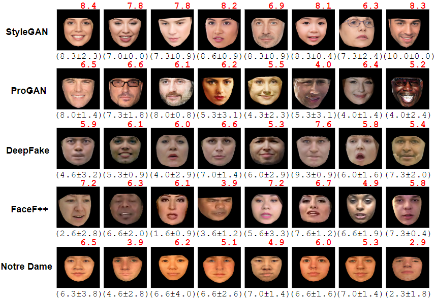
To further check the overall perceptual quality of each of the different synthesis approaches used in our study [51, 52, 2, 78, 9], we separately find the mean rating for each synthetic face image generated by that method, depicted in Figure 8. It comes as no surprise for the StyleGAN [52] images to rank the highest, with a mean score over 7, as its face images were pre-filtered for quality [4]. The other four approaches perform roughly the same, generating a mean score that falls between 6 and 7.
9 Quality Estimation Model: Loss Function
Our loss uses the L2 norm between the predicted quality () and mean label () and then computes a second L2 norm between this distance and the standard deviation (). acts as a margin in this case. If we consider as the center of a circle with radius of , then our loss tries to push towards the boundary to fully capture the subjectiveness of human perception. We also tried a hinge version of this loss: . This function penalizes falling outside the permissible circle while allowing it to lie anywhere within it. When is low, both functions act similarly. We found the quality estimation model’s () predictions to be less stochastic when trained with the margin loss than the hinge. On a held-out test set, both losses performed similarly with only 0.2% difference in regression accuracy. Experimental results with LEGAN, and especially StarGAN trained using (Tables 1, 2, 3 in the main text), underpin the efficiency of the margin loss in comprehending naturalness. The improvements in perceptual quality, as demonstrated by LPIPS and FID, further justify its validity as a good objective for training .
10 Quality Estimation Model: Prediction Accuracy During Testing
As discussed in Section 3 of the main text, we hold out 10% of the crowd-sourced data (3,727 face images) for testing our quality estimation model post training. Since never encountered these images during training, we use them to evaluate the effectiveness of our model. We separately compute the mean naturalness score for each synthesis approach used in our study and compare this value with the average quality score as predicted by . The results can be seen in Figure 9. Overall, our model predicts the naturalness score for each synthesis method with a high degree of certainty. Some qualitative results can also be seen in Figure 10.
11 LEGAN: Detailed Architecture
In this section, we list the different layers in the generator and discriminator of LEGAN. Since is composed of three hourglass networks, we separately describe their architecture in Tables 7, 8 and 9 respectively. The convolution layers, residual blocks and pixel shuffling layers are indicated as ‘conv’, ‘RB’, and ‘PS’ respectively in the tables. After each of ‘conv’ and ‘PS’ layer in an hourglass, we use ReLU activation and instance normalization [90], except for the last ‘conv’ layer where a tanh activation is used [77, 80]. The description of can be found in Table 10. Similar to , each convolution layer is followed by Leaky ReLU [99] activation with a slope of 0.01 in , except for the final two convolution layers that output the realness matrix and the classification map .

|
|
|
|
|
|
||||||
|---|---|---|---|---|---|---|---|---|---|---|---|
|
40.244 | 0.148 | 0.557 | 0.601 | 5.348 | ||||||
|
351.511 | 0.460 | 0.352 | 0.476 | 1.74 | ||||||
|
30.236 | 0.139 | 0.425 | 0.717 | 5.873 | ||||||
|
40.479 | 0.135 | 0.550 | 0.676 | 5.475 | ||||||
|
46.420 | 0.168 | 0.544 | 0.621 | 5.190 | ||||||
|
35.429 | 0.140 | 0.566 | 0.587 | 5.861 | ||||||
|
29.964 | 0.120 | 0.649 | 0.649 | 5.853 |
12 LEGAN: Ablation Study
To analyze the contribution of each loss component on synthesis quality, we prepare 5 different versions of LEGAN by removing (feature disentanglement, , , , , and ) from while keeping everything else the same. The qualitative and quantitative results, produced using MultiPIE [39] test data, are shown in Figure 11 and Table 11 respectively. For the quantitative results, the output image is compared with the corresponding target image in MultiPIE, and not the source image (\ieinput).
As expected, we find to be crucial for realistic hallucinations, in absence of which the model generates non-translated images totally outside the manifold of real images. The disentanglement of the lighting and expression via LEGAN’s hourglass pair allows the model to independently generate transformation masks which in turn synthesize more realistic hallucinations. Without the disentanglement, the model synthesizes face images with pale-ish skin color and suppressed expressions. When is removed, LEGAN outputs the input image back as the target attributes are not checked by anymore. Since the input image is returned back by the model, it generates a high face matching and mean quality score (Table 11, third row). When the reconstruction error is plugged off the output images lie somewhere in the middle, between the input and target expressions, suggesting the contribution of the loss in smooth translation of the pixels. Removing and deteriorates the overall naturalness, with artifacts manifesting in the eye and mouth regions. As expected, the overall best metrics are obtained when the full LEGAN model with all the loss components is utilized.
13 LEGAN: Optimal Upsampling
To check the effect of the different upsampling approaches on hallucination quality, we separately apply bilinear interpolation, transposed convolution [103] and pixel shuffling [82] on the decoder module of the three hourglass networks in LEGAN’s generator . While the upsampled pixels are interpolated based on the original pixel in the first approach, the other two approaches explicitly learn the possible intensity during upsampling. More specifically, pixel shuffling blocks learn the intensity for the pixels in the fractional indices of the original image (i.e. the upsampled indices) by using a set convolution channels and have been shown to generate sharper results than transposed convolutions. Unsurprisingly, it generates the best quantitative results by outperforming the other two upsampling approaches on 3 out of the 5 objective metrics, as shown in Table 12. Hence we use pixel shuffling blocks in our final implementation of LEGAN.
However, as can be seen in Figure 12, the expression and lighting transformation masks and are more meaningful when interpolated rather than explicitly learned. This interpolation leads to a smoother flow of upsampled pixels with facial features and their transformations visibly more noticeable compared to transposed convolutions and pixel shuffling.

|
|
|
|
|
|
||||||
|---|---|---|---|---|---|---|---|---|---|---|---|
|
29.933 | 0.128 | 0.630 | 0.653 | 5.823 | ||||||
|
28.585 | 0.125 | 0.635 | 0.644 | 5.835 | ||||||
|
29.964 | 0.120 | 0.649 | 0.649 | 5.853 |
14 LEGAN: Optimal Value of
As discussed in the main text, we set the value of the hyper-parameter = 8 for computing the quality loss . We arrive at this specific value after experimenting with different possible values. Since acts as a target for perceptual quality while estimating during the forward pass, it can typically range from 5 (realistic) to 10 (hyper-realistic). We set to all possible integral values between 5 and 10 for evaluating the synthesis results both qualitatively (Figure 13) and quantitatively (Table 13).

As can be seen, when is set to 8, LEGAN generates more stable images with much less artifacts compared to other values of . Also, the synthesized expressions are visibly more noticeable for this value of (Figure 13, top row). When evaluated quantitatively, images generated by LEGAN with = 8 garner the best score for 4 out of 5 objective metrics. This is interesting as setting = 10 (and not 8) should ideally generate hyper-realistic images and consequently produce the best quantitative scores. We attribute this behavior of LEGAN to the naturalness distribution of the images used to train our quality model . Since majority of these images fell in the (7-8) and (8-9) bins, and very few in (9-10) (as shown in Figure 7), ’s representations are aligned to this target. As a result, tends to rate hyper-realistic face images (i.e. images with mean naturalness rating between 8 - 10) with a score around 8. Such an example can be seen in the rightmost column of the first row in Figure 10, where rates a hyper-realistic StyleGAN generated image [52] as 8.3. Thus, setting = 8 for computation (using trained ’s weights) during LEGAN training produces the optimal results.
|
|
|
|
|
|
||||||
|---|---|---|---|---|---|---|---|---|---|---|---|
|
41.275 | 0.143 | 0.550 | 0.642 | 5.337 | ||||||
|
44.566 | 0.139 | 0.542 | 0.651 | 5.338 | ||||||
|
38.684 | 0.137 | 0.631 | 0.663 | 5.585 | ||||||
|
29.964 | 0.120 | 0.649 | 0.649 | 5.853 | ||||||
|
42.772 | 0.137 | 0.637 | 0.659 | 5.686 | ||||||
|
46.467 | 0.132 | 0.586 | 0.583 | 5.711 |

15 LEGAN: Perceptual Study Details
In this section, we share more details about the interface used for our perceptual study. As shown in Figure 14, we ask the raters to pick the image that best matches a target expression and lighting condition. To provide a basis for making judgement, we also share a real image of the same subject with neutral expression and bright lighting condition. However, this is not necessarily the input to the synthesis models for the target expression and lighting generation, as we want to estimate how these models do when the input image has more extreme expressions and lighting conditions. The image order is also randomized to eliminate any bias.
16 LEGAN: Model Limitations
Although LEGAN is trained on just frontal face images acquired in a controlled setting, it can still generate realistic new views even for non-frontal images with a variety of expressions, as shown in Figures 16 and 17. However, as with any synthesis model, LEGAN also has its limitations. In majority of the cases where LEGAN fails to synthesize a realistic image, the input expression is irregular with non-frontal head pose or occlusion, as can be seen in Figure 15. As a result, LEGAN fails to generalize and synthesizes images with incomplete translations or very little pixel manipulations. One way to mitigate this problem is to extend both our quality model and LEGAN to non-frontal facial poses and occlusions by introducing randomly posed face images during training.

17 LEGAN: More Qualitative Results
In this section, we share more qualitative results generated by LEGAN on unconstrained data from the AFLW [56] and CelebA [61] datasets in Figures 16 and 17 respectively. The randomly selected input images vary in ethnicity, gender, color composition, resolution, lighting, expression and facial pose. In order to judge LEGAN’s generalizability, we only train the model on 33k frontal face images from MultiPIE [39] and do not fine tune it on any other dataset.


18 Recolorization Network: Architecture Details
For the colorization augmentation network, we use a generator architecture similar to the one used in [10] for the 1281283 resolution. The generator is an encoder-decoder with skip connections connecting the encoder and decoder layers, and the discriminator is the popular CASIANet [101] architecture. Details about the generator layers can be found in Table 14.
|
|
|
|||
|---|---|---|---|---|---|
| conv0 | 33/1/2 | 128 | |||
| conv1 | 33/2/1 | 64 | |||
| RB1 | 33/1/1 | 64 | |||
| conv2 | 33/2/1 | 128 | |||
| RB2 | 33/1/1 | 128 | |||
| conv3 | 33/2/1 | 256 | |||
| RB3 | 33/1/1 | 256 | |||
| conv4 | 33/2/1 | 512 | |||
| RB4 | 33/1/1 | 512 | |||
| conv5 | 33/2/1 | 1,024 | |||
| RB5 | 33/1/1 | 1,024 | |||
| fc1 | 512 | - | |||
| fc2 | 16,384 | - | |||
| conv3 | 33/1/1 | 4*512 | |||
| PS1 | - | - | |||
| conv4 | 33/1/1 | 4*256 | |||
| PS2 | - | - | |||
| conv5 | 33/1/1 | 4*128 | |||
| PS3 | - | - | |||
| conv6 | 33/1/1 | 4*64 | |||
| PS4 | - | - | |||
| conv7 | 33/1/1 | 4*64 | |||
| PS5 | - | - | |||
| conv8 | 55/1/1 | 3 |

We train two separate versions of the colorization network with randomly selected 10,000 face images from the UMDFaces [12] and FFHQ [51] datasets. These two trained generators can then be used to augment LEGAN’s training set by randomly recoloring the MultiPIE [39] images from the training split. Such an example has been shared in Figure 18.