Least-squares formulations for Stokes equations with non-standard boundary conditions - A unified approach

S. Mohapatra^⋆, N. Kishore Kumar^†, Shivangi Joshi^† IIIT Delhi, Email: [email protected] Hyderabad Campus, Hyderabad, Email: [email protected] Hyderabad Campus, Hyderabad, Email: [email protected]

( )

Abstract

In this paper, we propose a unified non-conforming least-squares spectral element approach for solving Stokes equations with various non-standard boundary conditions. Existing least-squares formulations mostly deal with Dirichlet boundary conditions and are formulated using ADN theory based regularity estimates. However, changing boundary conditions lead to a search for parameters satisfying supplementing and complimenting conditions [4] which is not easy always. Here we have avoided ADN theory based regularity estimates and proposed a unified approach for dealing with various boundary conditions. Stability estimates and error estimates have been discussed. Numerical results displaying exponential accuracy have been presented for both two and three dimensional cases with various boundary conditions.

1 Introduction

Efficient numerical approximation of Stokes equations has been of great theoretical and computational interest for a long time as it is the first step to investigate nonlinear Navier Stokes equations. A search on numerical solutions of Stokes equations leads to an enormous amount of contributions. However, very few are available for Stokes equations with non-standard boundary conditions, i.e. boundary conditions other than Dirichlet. There are several practical instances like blood flow in arteries, water flow in pipes with bifurcation, oil ducts etc., which need to be analyzed other than velocity based Dirichlet boundary condition. A major challenge with changing the boundary conditions is to incorporate them in variational formulation and corresponding functional spaces.

Here we refer boundary conditions other than Dirichlet as non-standard boundary conditions and have listed eighteen different boundary conditions, being attached with Stokes differential operator from our literature survey. One common mathematical difficulty can be described as difficulty in understanding wellposedness of both continuous problem and discrete problem. Functional spaces need to be modified accordingly. Major difficulty with mixed finite element formulation with change in boundary conditions is to have appropriate saddle point formulation.

In this paper, we propose a unified approach for solving Stokes equations with various non-standard boundary conditions. The numerical scheme is based on a non-conforming least squares spectral element approach. Because of the least-squares formulation, the obtained linear system is always symmetric and positive definite in each case of boundary condition, hence we solve the linear system using the preconditioned conjugate gradient method. Minimization of least-squares functional consists of two parts. The first part consists of residues in differential operators and jumps in velocity and pressure components (along interelement boundaries). The second part consists of residues from the physical boundary conditions. This part varies with change in the boundary conditions. Norms are suitably chosen from available regularity estimates. Using the unified approach, any of these boundary conditions can be used with the Stokes problem and just boundary related terms need to be changed in the least-squares functional. No need to change in any other functional settings.

In section 2, we introduce Stokes equations with various non-standard boundary conditions, their physical motivations, theoretical, computational developments and available regularity estimates. Stability estimates for numerical solutions have been discussed in section 3. Numerical schemes have been discussed in section 4. Error estimates are discussed in section 5. Numerical results with some of these boundary conditions have been presented in section 6. Finally, we conclude with section 7.

2 Notations

Let $\Omega\subset\mathbb{R}^{n},n=2,3$ with sufficiently smooth boundary $\Gamma=\partial\Omega$ . Here we consider the Stokes system

\displaystyle\begin{cases}-\Delta\mbox{\boldmath$u$}+\nabla p=\mbox{\boldmath$f$}\quad\mbox{in}\quad\Omega,\\ -\nabla\cdot\mbox{\boldmath$u$}=\chi\quad\mbox{in}\quad\Omega\\ \end{cases}

(1)

with different boundary conditions other than just Dirichlet boundary conditions. Basic least-squares formulation leads to minimize the residuals in differential operators and residuals in boundary conditions in appropriate norms ([47], [48], [49], [38], [30], [22], [23],[39],[43],[44], [26],[27], [37]).

Let’s denote $\mathcal{L}(\mbox{\boldmath$u$},p)=-\Delta\mbox{\boldmath$u$}+\nabla p,\mathcal{D}\mbox{\boldmath$u$}=-\nabla\cdot\mbox{\boldmath$u$}$ . Let $\mbox{\boldmath$n$}=(n_{1},n_{2}),(n_{1},n_{2},n_{3})$ be the unit outward normal to $\Gamma=\partial\Omega$ for $\Omega\subset{\mathbb{R}}^{2},{\mathbb{R}}^{3}$ respectively. $u_{\mbox{\boldmath$n$}}=\mbox{\boldmath$u$}.\mbox{\boldmath$n$},\mbox{\boldmath$u$}_{\tau}=\mbox{\boldmath$u$}-\mbox{\boldmath$n$}u_{\mbox{\boldmath$n$}}$ denote the normal and tangential components of the velocity. $\sigma_{\mbox{\boldmath$n$}}=\sigma_{\mbox{\boldmath$n$}}(\mbox{\boldmath$u$},p)=\sigma(\mbox{\boldmath$u$},p).\mbox{\boldmath$n$},\sigma_{\mbox{\boldmath$\tau$}}=\sigma_{\mbox{\boldmath$\tau$}}(\mbox{\boldmath$u$},p)=\sigma(\mbox{\boldmath$u$},p)-\mbox{\boldmath$n$}\sigma_{\mbox{\boldmath$n$}}(\mbox{\boldmath$u$},p)$ denote normal and tangential components of stress vector. Here $\sigma(\mbox{\boldmath$u$},p)=(-p\delta_{ij}+e_{ij}\mbox{\boldmath$u$})\mbox{\boldmath$n$},e_{ij}(\mbox{\boldmath$u$})=\frac{\partial u_{i}}{\partial x_{j}}+\frac{\partial u_{j}}{\partial x_{i}}$ . $\mathbb{D}(\mbox{\boldmath$u$})=\frac{1}{2}(\nabla\mbox{\boldmath$u$}+\nabla\mbox{\boldmath$u$}^{T})$ denotes the strain tensor. Let’s denote $L^{2}(\Omega)/{\mathbb{R}}=\left\{q\in L^{2}(\Omega)\mathrel{\mathop{\mathchar 58\relax}}\int_{\Omega}qd\Omega=0\right\}.$ $c$ is treated as a generic constant, which has different values with different situations.

$H^{m}(\Omega)$ denotes the Sobolev space of functions with square integrable derivatives of integer order less than or equal to $m$ on $\Omega$ equipped with the norm

\displaystyle{\|u\|}_{H^{m}(\Omega)}^{2}=\sum_{\left|\alpha\right|\leq m}{\|D^{\alpha}u\|}_{{L^{2}(\Omega)}^{2}}.

Further, let $E=(-1,1)^{d-1}$ . Then we define fractional norms $(0<\mu<1)$ by :

•

if $\Gamma_{l}\in\partial\Omega\!\!\!\quad\mbox{when}\quad\!\!\!\Omega\subset\mathbb{R}^{2}$

\displaystyle\left\|u\right\|_{\mu,\Gamma_{l}}^{2}=\|u\|_{0,E}^{2}+\int_{E}\int_{E}\frac{\left|u(\xi)-u(\xi^{\prime})\right|^{2}}{\left|\xi-\xi^{\prime}\right|^{1+2\mu}}d\xi d\xi^{\prime}.

•

if $\Gamma_{l}\in\partial\Omega\!\!\!\quad\mbox{when}\quad\!\!\!\Omega\subset\mathbb{R}^{3}$

	$\displaystyle\\|u\\|_{\mu,\Gamma_{l}}^{2}=\\|u\\|_{0,E}^{2}+\int_{E}\int_{E}\int_{E}\frac{(u(\xi,\eta)-u(\xi^{\prime},\eta))^{2}}{(\xi-\xi^{\prime})^{1+2\mu}}\,d\xi d\xi^{\prime}d\eta$
	$\displaystyle+\int_{E}\int_{E}\int_{E}\frac{(u(\xi,\eta)-u(\xi,\eta^{\prime}))^{2}}{(\eta-\eta^{\prime})^{1+2\mu}}\,d\eta d\eta^{\prime}d\xi\,.$

We denote the vectors by bold letters. For example if $\Omega\subset\mathbb{R}^{2}$ , $\mbox{\boldmath$u$}=(u_{1},u_{2})^{T}$ , $\mbox{\boldmath$H$}^{k}(\Omega)=H^{k}(\Omega)\times H^{k}(\Omega)$ , $\|\mbox{\boldmath$u$}\|_{k,\Omega}^{2}=\|u_{1}\|_{k,\Omega}^{2}+\|u_{2}\|_{k,\Omega}^{2}$ etc.. We define the functional spaces and norms similarly for three dimensional case.

Next, we present different boundary conditions existing in the literature that have been encountered with Stokes equations in various physical applications. We plan to discuss exponentially accurate least-squares spectral element formulations for Stokes equations with each of these boundary conditions.

•

(B1) $\Gamma=\bar{\Gamma}_{1}\cup\bar{\Gamma}_{2}$

\displaystyle\begin{cases}\mbox{\boldmath$u$}=\mbox{\boldmath$g$}\quad\!\!\!\mbox{on}\quad\!\!\!\Gamma_{1}\\ \mbox{\boldmath$u$}.\mbox{\boldmath$n$}=\mbox{\boldmath$g$}_{\mbox{\boldmath$n$}},(\nabla\times\mbox{\boldmath$u$})\times\mbox{\boldmath$n$}=\mbox{\boldmath$k$}\times\mbox{\boldmath$n$}\quad\!\!\!\mbox{on}\quad\!\!\!\Gamma_{2}\end{cases}(\cite[cite]{[\@@bibref{}{AM7}{}{}]})

•

(B2) $\mbox{\boldmath$u$}_{\mbox{\boldmath$n$}}=\mbox{\boldmath$g$}_{\mbox{\boldmath$n$}},[\frac{\partial\mbox{\boldmath$u$}}{\partial\mbox{\boldmath$n$}}-p\mbox{\boldmath$n$}+b\mbox{\boldmath$u$}]_{\mbox{\boldmath$\tau$}}=\mbox{\boldmath$h$}_{\mbox{\boldmath$\tau$}}$ on $\Gamma$ ([40],[41])
•

(B3) $\mbox{\boldmath$u$}_{\mbox{\boldmath$n$}}=\mbox{\boldmath$g$}_{\mbox{\boldmath$n$}},\big{(}[\nabla\mbox{\boldmath$u$}+(\nabla\mbox{\boldmath$u$})^{T}-pI]\mbox{\boldmath$n$}+b\mbox{\boldmath$u$}\big{)}_{\mbox{\boldmath$\tau$}}=\mbox{\boldmath$h$}_{\mbox{\boldmath$\tau$}}$ on $\Gamma$ ([40],[41])
•

(B4) $\mbox{\boldmath$u$}.\mbox{\boldmath$n$}=g$ , $(\nabla\times\mbox{\boldmath$u$})\times\mbox{\boldmath$n$}=\mbox{\boldmath$h$}\times\mbox{\boldmath$n$}$ on $\Gamma$ ([7],[9],[24])
•

(B5) $\mbox{\boldmath$u$}\times\mbox{\boldmath$n$}=\mbox{\boldmath$g$}\times\mbox{\boldmath$n$},p=\tilde{p}$ on $\Gamma$ ([8],[9])

•

(B6) $\Gamma=\bar{\Gamma}_{1}\cup\bar{\Gamma}_{2}\cup\bar{\Gamma}_{3}$

\displaystyle\begin{cases}\mbox{\boldmath$u$}=\mbox{\boldmath$u$}_{0}\quad\!\!\mbox{on}\quad\!\!\Gamma_{1},\\ \mbox{\boldmath$u$}\times\mbox{\boldmath$n$}=\mbox{\boldmath$a$}\times\mbox{\boldmath$n$},p=p_{0}\quad\!\!\mbox{on}\quad\!\!\Gamma_{2},\\ \mbox{\boldmath$u$}.\mbox{\boldmath$n$}=\mbox{\boldmath$b$}.\mbox{\boldmath$n$},(\nabla\times\mbox{\boldmath$u$})\times\mbox{\boldmath$n$}=\mbox{\boldmath$h$}\times\mbox{\boldmath$n$}\quad\!\!\mbox{on}\quad\!\!\Gamma_{3}\end{cases}(\cite[cite]{[\@@bibref{}{CO1}{}{}]},\cite[cite]{[\@@bibref{}{BE1}{}{}]},\cite[cite]{[\@@bibref{}{CO2}{}{}]})

•

(B7) $\mbox{\boldmath$u$}.\mbox{\boldmath$n$}=g,[(2\mathbb{D}\mbox{\boldmath$u$})\mbox{\boldmath$n$}]_{\mbox{\boldmath$\tau$}}=\mbox{\boldmath$h$}\quad\!\!\mbox{on}\quad\!\!\Gamma$ ([3], [8])
•

(B8) $\mbox{\boldmath$u$}.\mbox{\boldmath$n$}=0,(\nabla\times\mbox{\boldmath$u$})_{\mbox{\boldmath$\tau$}}=0\quad\!\!\mbox{on}\quad\!\!\Gamma$ ([18])

•

(B9) $\Gamma=\bar{\Gamma}_{1}\cup\bar{\Gamma}_{2}$

\displaystyle\begin{cases}\mbox{\boldmath$u$}=\mbox{\boldmath$g$}\quad\!\!\!\mbox{on}\quad\!\!\!\Gamma_{1},\\ p=\phi,\mbox{\boldmath$u$}\times\mbox{\boldmath$n$}=\tilde{g}\quad\!\!\!\mbox{on}\quad\!\!\!\Gamma_{2}\end{cases}(\cite[cite]{[\@@bibref{}{BE2}{}{}]})

•

(B10) $\big{(}(\nu\nabla\mbox{\boldmath$u$}-pI)\mbox{\boldmath$n$}\big{)}.\mbox{\boldmath$n$}=\mbox{\boldmath$g$}\quad\!\!\!\mbox{on}\quad\!\!\!\Gamma,\mbox{\boldmath$u$}_{\mbox{\boldmath$\tau$}}=0\quad\!\!\!\mbox{on}\quad\!\!\!\Gamma$ ([12])
•

(B11) $\mbox{\boldmath$u$}.\mbox{\boldmath$n$}=0,\nabla\times\mbox{\boldmath$u$}=0\quad\!\!\!\mbox{on}\quad\!\!\!\Gamma$ ([45])

•

(B12) $\Gamma=\bar{\Gamma}_{1}\cup\bar{\Gamma}_{2}\cup\bar{\Gamma}_{3}$

\displaystyle\begin{cases}\mbox{\boldmath$u$}=\mbox{\boldmath$u$}_{0}=(u_{01},u_{02})\quad\!\!\!\mbox{on}\quad\!\!\!\Gamma_{1},\\ \mbox{\boldmath$u$}\times\mbox{\boldmath$n$}=u_{02},p=\phi\quad\!\!\!\mbox{on}\quad\!\!\!\Gamma_{2},\\ \mbox{\boldmath$u$}.\mbox{\boldmath$n$}=u_{01},(\nabla\times\mbox{\boldmath$u$}).\mbox{\boldmath$\tau$}=\mbox{\boldmath$h$}\quad\!\!\!\mbox{on}\quad\!\!\!\Gamma_{3}\end{cases}\cite[cite]{[\@@bibref{}{BE4}{}{}]}

•

(B13) $\Gamma=\bar{\Gamma}_{1}\cup\bar{\Gamma}_{2}\cup\bar{\Gamma}_{3}$

\displaystyle\begin{cases}\mbox{\boldmath$u$}=\mbox{\boldmath$g$}\quad\!\!\!\mbox{on}\quad\!\!\!\Gamma_{1},\\ \mbox{\boldmath$n$}.\mbox{\boldmath$u$}=\mbox{\boldmath$g$}_{n},\mbox{\boldmath$n$}\times((\nabla\times\mbox{\boldmath$u$})\times\mbox{\boldmath$n$})=\mbox{\boldmath$w$}_{s}\quad\!\!\!\mbox{on}\quad\!\!\!\Gamma_{2},\\ p=\psi,\mbox{\boldmath$n$}\times(\mbox{\boldmath$u$}\times\mbox{\boldmath$n$})=\mbox{\boldmath$g$}_{s}\quad\!\!\!\mbox{on}\quad\!\!\!\Gamma_{3},\\ p=\psi,\mbox{\boldmath$n$}\times((\nabla\times\mbox{\boldmath$u$})\times\mbox{\boldmath$n$})=\mbox{\boldmath$g$}_{s}\quad\!\!\!\mbox{on}\quad\!\!\!\Gamma_{4}\end{cases}(\cite[cite]{[\@@bibref{}{HU1}{}{}]})

•

(B14) $\Gamma=\bar{\Gamma}_{0}\cup\bar{\Gamma}_{1}$

\displaystyle\begin{cases}\mbox{\boldmath$u$}=0\quad\!\!\!\mbox{on}\quad\!\!\!\Gamma_{0},\\ \mbox{\boldmath$u$}_{\mbox{\boldmath$\tau$}}=0,\sigma_{\mbox{\boldmath$n$}}=\omega_{\mbox{\boldmath$n$}}\quad\!\!\!\mbox{on}\quad\!\!\!\Gamma_{1}\end{cases}(\cite[cite]{[\@@bibref{}{SA1}{}{}]})

•

(B15) $\Gamma=\bar{\Gamma}_{0}\cup\bar{\Gamma}_{1}$

\displaystyle\begin{cases}\mbox{\boldmath$u$}=0\quad\!\!\!\mbox{on}\quad\!\!\!\Gamma_{0},\\ \mbox{\boldmath$u$}_{\mbox{\boldmath$n$}}=0,\sigma_{\mbox{\boldmath$\tau$}}=\omega_{\mbox{\boldmath$\tau$}}\quad\!\!\!\mbox{on}\quad\!\!\!\Gamma_{1}\end{cases}(\cite[cite]{[\@@bibref{}{SA1}{}{}]})

•

(B16) $\mbox{\boldmath$u$}.\mbox{\boldmath$n$}=g,\nu{\mbox{\boldmath$u$}}_{\mbox{\boldmath$\tau$}}+{[\sigma(\mbox{\boldmath$u$},p).\mbox{\boldmath$n$}]}_{\mbox{\boldmath$\tau$}}=\mbox{\boldmath$s$}\quad\!\!\!\mbox{on}\quad\!\!\!\Gamma$ ([50], [60])
•

(B17) $\mbox{\boldmath$u$}.\mbox{\boldmath$\tau$}=g,p=h\quad\!\!\!\mbox{on}\quad\!\!\!\Gamma$ ([40])
•

(B18) $\mbox{\boldmath$u$}.\mbox{\boldmath$n$}=g,{[(2\mathbb{D}\mbox{\boldmath$u$})\mbox{\boldmath$n$}]}_{\mbox{\boldmath$\tau$}}+\alpha{\mbox{\boldmath$u$}}_{\mbox{\boldmath$\tau$}}=\mbox{\boldmath$h$}\quad\!\!\!\mbox{on}\quad\!\!\!{\Gamma}$ ([10],[55])

Remark 2.1.

Here we have not mentioned the regularity of the domains in detail. However, information related to each boundary condition can be traced from the given references. For proposing the numerical schemes, we assume that the boundary of computational domains have the necessary regularity.

2.1 Motivations and physical applications

Here we discuss physical applications of some of the boundary conditions. Stokes equations with boundary conditions of type (B1) are encountered in many physical problems such as a tank closed with a membrane on a part of the boundary, coupling with different equations such as Darcy’s equations in the case of fluid domain is with a crack in a porus medium ([19],[20]). Use of (B4) in Stokes equations help to design variational formulations without $p$ term. The boundary conditions arise in fluid dynamics related applications, electromagnetic field applications, decomposition of vector fields ([13], [14], [31], [34],[59]). Stokes equations with boundary conditions on tangential component of velocity and pressure boundary conditions (B5) are encountered in many physical applications such as Stokes equations in pipelines [28] and blood vessels ([61],[62],[57],[46],[35]). Boundary conditions of type (B6) are encountered in case of flow network in pipes, obstacles in pipes, modeling boundary conditions for infinite flow around obstacle etc. [29]. Stokes equations with boundary conditions of type (B7) are used in understanding the coupling problem of Stokes and Darcy equations, which has immense importance in geophysical systems. The difficulty arises because of the large difference in scales between the porous media and the cracks where the flow is quite faster. Apart from cracks, such coupling problems have applications in seepage of water in sand e.g. from lake to ground, from sea to sands in the beach. Stokes equations with boundary conditions ((B2), (B3), (B16), (B18)) are called slip boundary conditions [58] and are used in modelling of flow problems with free boundaries ( e.g. coating problem [53]), flows past chemically reacting walls and flow problems where no-slip boundary conditions are not valid, incompressible viscous flows with high angles of attack and high Reynold’s numbers. In the case of free surface problems [54], use of no-slip condition on the fixed part of the boundary leads to stress singularities. This is regarded as a case of nonphysical singularity and disappears with use of slip boundary conditions near the solid free surface contact point. Stokes equations with boundary conditions of type (B9) can be treated as generalization of Poiseuille flow in a channel, where $\Gamma_{1}$ represents the rigid wall and inflow/outflow takes place through $\Gamma_{2}$ . Boundary conditions of type (B14) refers to fluid under investigation does not slip at the boundary and penetration of fluid through the boundary is controlled by the normal component of stress.

2.2 Theoretical developments on Stokes equations with non-standard boundary conditions

Next, we briefly discuss existing theoretical results on Stokes equations with various non-standard boundary conditions. These results help us in formulating numerical schemes in appropriate functional spaces. Medkova [40] has studied Stokes equations with three different boundary conditions (B2), (B3), (B4) named as of Navier type on two dimensional bounded domains with Lipschitz boundary. Necessary and sufficient conditions for the existence of solutions on planar domains in Sobolev spaces and Besov spaces have been obtained. Amrouche et. al. [9] have studied Stokes equations with boundary conditions (B4),(B5) on three dimensional $C^{1,1}$ bounded multiply connected domains. Existence, uniqueness results of weak, strong and very weak solutions have been provided. Amrouche et. al. [10] have theoretically studied Stokes equations with boundary conditions (B18) with zero boundary data. Existence, uniqueness and regularity estimates on different Sobolev spaces have been provided. Abboud et. al. ([1],[2]) have studied Stokes equations with boundary conditions (B4) and (B5) with homogeneous boundary data on three dimensional bounded, simply connected domains. Proposed variational formulation decouples the original problem into a system of velocity and a Poisson problem for pressure. A priori and a posteriori estimates have been obtained and confirmed with numerical results. A finite element formulation has been used for theoretical and numerical results. Bernard [15] has analyzed Stokes equations and Navier-Stokes equations with boundary conditions (B6) for three dimensional bounded domains with boundary of class $C^{1,1}.$ Existence, uniqueness, and regularity estimates have been obtained in various Sobolev spaces. Results obtained are applicable for two dimensional domains too, with suitable modification. Acvedo et. al. [3] have studied Stokes operator with boundary conditions (B7) on three dimensional bounded $C^{1,1}$ domains. Existence, uniqueness and regularity results have been obtained in different Sobolev spaces. Bramble and Lee [24] have investigated Stokes equations with boundary conditions (B4) on three dimensional bounded domains. The existence, uniqueness results and a general shift theorem have been provided. Existence and uniqueness results of variational formulation for Stokes equations with boundary condition (B6) have been discussed in [29]. Medkova [41] has discussed solvability issues of the Stokes system with (B17) in Sobolev and Besov spaces.

2.3 Computational developments on Stokes equations with non-standard boundary conditions

A spectral approximation of Stokes equations with boundary condition (B9) has been investigated in [17]. A stabilized hybrid discontinuous Galerkin approach using finite elements has been used for Stokes equations with boundary conditions (B10) [12]. Bernardi and Chorfi [18] has discussed a spectral formulation for vorticity based first order formulation of Stokes equations with boundary condition (B8). Numerical results suppporting theoretical estimates have been presented. Bernard [16] has presented a spectral discretization (without numerical results) for Stokes equations with boundary conditions (B12). Amara et. al. [5] have discussed vorticity-velocity-pressure formulation for Stokes problem with boundary conditions (B13) where $w=\nabla\times\mbox{\boldmath$u$},\Gamma={\overline{\Gamma}}_{1}\cup{\overline{\Gamma}}_{2}\cup{\overline{\Gamma}}_{3}$ on two dimensional domains with assumptions that there is no non-convex corner at the intersection of ${\overline{\Gamma}}_{1}\cup{\overline{\Gamma}}_{2}$ and ${\overline{\Gamma}}_{3}$ . Conca et. al. [28] have presented a variational formulation for Stokes equations with boundary condition (B6). Authors have extended results for Navier-Stokes equations. Optimal, a priori error estimates for Stokes equations with boundary conditions (B4) and (B5) with homogeneous data on three dimensional domains have been presented in [1]. Hughes [36] has presented convergent symmetric finite element formulations for Stokes equations with (B13). Authors [21] have discussed Stokes equations with pressure boundary condition, (B5) on two and three dimensional domains. Convergence analysis and numerical simulations have been presented. A spectral discretization for vorticity based first order formulation of Stokes equations with (B4) has been discussed in [6].

Remark 2.2.

Development of computational aspects of Stokes equations with various non-standard boundary conditions is displayed in Table 1. Following table says no unified approach exists in the literature to accomodate so many boundary conditions. Also least-squares formulations have not been used. Hence least-squares approach to deal with various non-standard boundary condtions in a unified framework is the key achievement of this paper.

B.C.	Method	Numerical results	2D/3D	Extn to NS	Ref
(B4)/(B5)	Finite element	Yes	3D	No	[1]
(B4)	Spectral Galerkin	Yes	2D $\&$ 3D	No	[6]
(B5)	Finite element	Yes	2D $\&$ 3D	No	[21]
(B6)	Finite element	Yes	2D $\&$ 3D	Yes	[28]
(B8)	Spectral Galerkin	Yes	2D $\&$ 3D	No	[18]
(B9)	Spectral Galerkin	No	2D	No	[17]
(B10)	Stabilized DGFEM	Yes	2D	No	[12]
(B12)	Spectral Galerkin	No	2D	No	[16]
(B13)	Finite element	Yes	2D	No	[5]
(B13)	Finite element	No	2D $\&$ 3D	No	[36]

Table 1: Summary of computational developments

2.4 Regularity for $(\mbox{\boldmath$u$},p)$ in Stokes equations with various non-stanadard boundary conditions

We need regularity estimates of $\mbox{\boldmath$H$}^{2}$ and $H^{1}$ type for velocity and pressure variable respectively to propose the numerical schemes. In this section we discuss regularity estimates for Stokes equations with different boundary conditions.

•

Regularity for Stokes equations with (B4) [9]
If $\mbox{\boldmath$f$}\in\mbox{\boldmath$L$}^{2}(\Omega),g\in H^{\frac{3}{2}}(\Gamma),\mbox{\boldmath$h$}\in\mbox{\boldmath$H$}^{\frac{1}{2}}(\Gamma)$ , the solution $(\mbox{\boldmath$u$},p)\in\mbox{\boldmath$H$}^{2}(\Omega)\times H^{1}(\Omega)$ and satisfies

\displaystyle\|\mbox{\boldmath$u$}\|_{\mbox{\boldmath$H$}^{2}(\Omega)}+\|p\|_{H^{1}(\Omega)}\leq c\big{(}\|\mbox{\boldmath$f$}\|_{\mbox{\boldmath$L$}^{2}(\Omega)}+\|g\|_{H^{\frac{3}{2}}(\Gamma)}+\|\mbox{\boldmath$h$}\times\mbox{\boldmath$n$}\|_{\mbox{\boldmath$H$}^{\frac{1}{2}}(\Gamma)}\big{)}.

•

Regularity for Stokes equations with (B5) [9]
If $\mbox{\boldmath$f$}\in\mbox{\boldmath$L$}^{2}(\Omega),\mbox{\boldmath$g$}\in\mbox{\boldmath$H$}^{\frac{3}{2}}(\Gamma),\tilde{p}\in H^{\frac{1}{2}}(\Gamma)$ , the solution $(\mbox{\boldmath$u$},p)\in\mbox{\boldmath$H$}^{2}(\Omega)\times H^{1}(\Omega)$ and satisfies

\displaystyle\|\mbox{\boldmath$u$}\|_{\mbox{\boldmath$H$}^{2}(\Omega)}+\|p\|_{H^{1}(\Omega)}\leq c\big{(}\|\mbox{\boldmath$f$}\|_{\mbox{\boldmath$L$}^{2}(\Omega)}+\|\mbox{\boldmath$g$}\times\mbox{\boldmath$n$}\|_{\mbox{\boldmath$H$}^{\frac{1}{2}}(\Gamma)}+\|\tilde{p}\|_{H^{\frac{1}{2}}(\Gamma)}\big{)}.

•

Regularity for Stokes equations with (B6) [15]
If $\mbox{\boldmath$f$}\in\mbox{\boldmath$L$}^{2}(\Omega),\mbox{\boldmath$u$}_{0}\in\mbox{\boldmath$H$}^{\frac{3}{2}}(\Gamma_{1}),\mbox{\boldmath$a$}\in\mbox{\boldmath$H$}^{\frac{3}{2}}(\Gamma_{2}),p_{0}\in H^{\frac{1}{2}}(\Gamma_{2}),$ $\mbox{\boldmath$b$}\in\mbox{\boldmath$H$}^{\frac{3}{2}}(\Gamma_{3}),\mbox{\boldmath$h$}\in\mbox{\boldmath$H$}^{\frac{1}{2}}(\Gamma_{3})$ then Stokes equations with boundary conditions (B6) has a solution of the form $(\mbox{\boldmath$u$}+\mbox{\boldmath$w$},p)$ with $\mbox{\boldmath$w$}\in V_{1}$ , where $V_{1}=\left\{\mbox{\boldmath$v$}\in V\mathrel{\mathop{\mathchar 58\relax}}\nabla\times\mbox{\boldmath$v$}=0\right\}$ , satisfying the regularity estimate

\displaystyle\inf_{\mbox{\boldmath$w$}\in V_{1}}\|\mbox{\boldmath$u$}+\mbox{\boldmath$w$}\|_{\mbox{\boldmath$H$}^{2}(\Omega)}+\|p\|_{H^{1}(\Omega)}\leq c\big{(}\|\mbox{\boldmath$f$}\|_{\mbox{\boldmath$L$}^{2}(\Omega)}+\|\mbox{\boldmath$u$}_{0}\|_{\mbox{\boldmath$H$}^{\frac{3}{2}}(\Gamma_{1})}+\|\mbox{\boldmath$a$}\|_{\mbox{\boldmath$H$}^{\frac{3}{2}}(\Gamma_{1})}\big{)}.

•

Regularity for Stokes equations with (B7) [8]
If $\mbox{\boldmath$f$}\in\mbox{\boldmath$L$}^{p}(\Omega),\chi\in H^{1}(\Omega),g\in H^{\frac{3}{2}}(\Gamma),\mbox{\boldmath$h$}\in\mbox{\boldmath$H$}^{\frac{1}{2}}(\Gamma)$ satisfy compatibility conditions (Theorem 4.1, [8]), then Stokes equations with boundary conditions (B7) has a unique solution $(\mbox{\boldmath$u$},p)\in(\mbox{\boldmath$H$}^{2}(\Omega)\times H^{1}(\Omega))/\mathcal{N}(\Omega)$ satisfying

\displaystyle\|\mbox{\boldmath$u$}\|_{\mbox{\boldmath$H$}^{2}(\Omega)/\mathcal{T}(\Omega)}+\|p\|_{H^{1}(\Omega)/\mathbb{R}}\leq c\big{(}\|\mbox{\boldmath$f$}\|_{\mbox{\boldmath$L$}^{2}(\Omega)}+\|g\|_{H^{\frac{3}{2}}(\Gamma)}+\|\mbox{\boldmath$h$}\|_{\mbox{\boldmath$H$}^{\frac{1}{2}}(\Gamma)}\big{)},

where

	$\displaystyle\mathcal{T}(\Omega)=\left\{\mbox{\boldmath$u$}\in\mbox{\boldmath$H$}^{1}(\Omega)\mathrel{\mathop{\mathchar 58\relax}}\mathbb{D}\mbox{\boldmath$u$}=0\quad\!\!\!\mbox{in}\quad\!\!\!\Omega,\nabla.\mbox{\boldmath$u$}=0\quad\!\!\!\mbox{in}\quad\!\!\!\Omega,\mbox{\boldmath$u$}.\mbox{\boldmath$n$}=0\quad\!\!\!\mbox{on}\quad\!\!\!\Gamma\right\}$
	$\displaystyle\mathcal{N}(\Omega)=\left\{(\mbox{\boldmath$u$},c)\mathrel{\mathop{\mathchar 58\relax}}\mbox{\boldmath$u$}\in\mathcal{T}(\Omega),c\in\mathbb{R}\right\}.$

•

Regularity for Stokes equations with (B11) [45]
If $\mbox{\boldmath$f$}\in\mbox{\boldmath$L$}^{2}(\Omega),\chi\in H^{1}(\Omega)\cap L^{2}/(\mathbb{R})$ , then Stokes equations with (B11) has a unique solution $(\mbox{\boldmath$u$},p)\in\mbox{\boldmath$H$}^{2}(\Omega)\times H^{1}(\Omega)$ satisfying

\displaystyle\|\mbox{\boldmath$u$}\|_{\mbox{\boldmath$H$}^{2}(\Omega)}+\|p\|_{H^{1}(\Omega)}\leq c\big{(}\|\mbox{\boldmath$f$}\|_{\mbox{\boldmath$L$}^{2}(\Omega)}+\|\chi\|_{\mbox{\boldmath$H$}^{1}(\Omega)}\big{)}.

•

Regularity for Stokes equations with (B14) [52]
For $\mbox{\boldmath$f$}\in\mbox{\boldmath$L$}^{2}(\Omega),\omega_{\mbox{\boldmath$n$}}\in\mbox{\boldmath$H$}^{\frac{1}{2}}(\Gamma)$ . If $(\mbox{\boldmath$u$},p)$ are the weak solutions, then $\mbox{\boldmath$u$}\in\mbox{\boldmath$H$}^{2}(\Omega),p\in H^{1}(\Omega)$ satisfying the inequality

\displaystyle\|\mbox{\boldmath$u$}\|_{\mbox{\boldmath$H$}^{2}(\Omega)}+\|p\|_{H^{1}(\Omega)}\leq c\big{(}\|\mbox{\boldmath$f$}\|_{\mbox{\boldmath$L$}^{2}(\Omega)}+\|\omega_{\mbox{\boldmath$n$}}\|_{\frac{1}{2},\Gamma}\big{)}.

•

Regularity for Stokes equations with (B15) [52]
For $\mbox{\boldmath$f$}\in\mbox{\boldmath$L$}^{2}(\Omega),\omega_{\mbox{\boldmath$\tau$}}\in\mbox{\boldmath$H$}^{\frac{1}{2}}(\Gamma)$ , we have $\mbox{\boldmath$u$}\in\mbox{\boldmath$H$}^{2}(\Omega),p\in H^{1}(\Omega)$ satisfying the inequality

\displaystyle\|\mbox{\boldmath$u$}\|_{\mbox{\boldmath$H$}^{2}(\Omega)}+\|p\|_{H^{1}(\Omega)}\leq c\big{(}\|\mbox{\boldmath$f$}\|_{\mbox{\boldmath$L$}^{2}(\Omega)}+\|\omega_{\mbox{\boldmath$\tau$}}\|_{\frac{1}{2},\Gamma}\big{)}.

•

Regularity of Stokes equations with boundary conditions (B18) [55]

For $\mbox{\boldmath$f$}\in\mbox{\boldmath$L$}^{2}(\Omega),\mbox{\boldmath$h$}\in\mbox{\boldmath$H$}^{\frac{1}{2}}(\Gamma),(\mbox{\boldmath$u$},p)\in\mbox{\boldmath$H$}^{2}(\Omega)\times H^{1}(\Omega)$

\displaystyle\|\mbox{\boldmath$u$}\|_{\mbox{\boldmath$H$}^{2}(\Omega)}+\|p\|_{H^{1}(\Omega)}\leq c\big{(}\|\mbox{\boldmath$f$}\|_{\mbox{\boldmath$L$}^{2}(\Omega)}+\|\mbox{\boldmath$h$}\|_{\mbox{\boldmath$H$}^{\frac{1}{2}}(\Gamma)}\big{)}.

Remark 2.3.

Similar regularity estimates are missing in the literature for some of the boundary conditions. However, we assume that boundary data of Dirichlet type for velocity is in $\mbox{\boldmath$H$}^{\frac{3}{2}}(\Gamma)$ and pressure is in $H^{\frac{1}{2}}(\Gamma)$ .

3 Stability estimates

In this section, we prove the stability estimates for Stokes problem with (B4) and (B5). Stability estimates in other boundary cases can be derived in a similar way. We denote $\mbox{\boldmath$x$}=(x_{1},x_{2})$ and $\mbox{\boldmath$x$}=(x_{1},x_{2},x_{3})$ if $\mbox{\boldmath$x$}\in\Omega\subset\mathbb{R}^{n},n=2,3$ respectively. $\Omega$ is divided into $L$ number of subdomains. For simplicity, $\Omega_{l}$ ’s are chosen to be rectangles in $\mathbb{R}^{2}$ and cubes in $\mathbb{R}^{3}$ respectively. Let $Q$ denote the master element $Q=(-1,1)^{n},n=2,3$ . Now there is an analytic map $M_{l}$ from $\Omega_{l}$ to $Q$ which has an analytic inverse. The map $M_{l}$ is of the form $\hat{}\mbox{\boldmath$x$}=M_{l}({\mbox{\boldmath$x$}})$ , where $\hat{\mbox{\boldmath$x$}}=(\xi,\eta)$ and $\hat{\mbox{\boldmath$x$}}=(\xi,\eta,\nu)$ if $\Omega\subset\mathbb{R}^{d},d=2,3$ respectively. Define the non-conforming spectral element functions $\mbox{\boldmath$u$}_{l}$ and $p_{l}$ on $Q$ by

•

if $\Omega_{l}\subseteq\Omega\subset{\mathbb{R}}^{2}$

\displaystyle\hat{\mbox{\boldmath$u$}}|_{Q}(\xi,\eta)=\sum_{i=0}^{W}\sum_{j=0}^{W}\mathbf{a}_{i,j}\>\xi^{i}\eta^{j},\quad\hat{p}|_{Q}(\xi,\eta)=\sum_{i=0}^{W}\sum_{j=0}^{W}b_{i,j}\xi^{i}\eta^{j}.

•

if $\Omega_{l}\subseteq\Omega\subset{\mathbb{R}}^{3}$

\displaystyle\hat{\mbox{\boldmath$u$}}|_{Q}(\xi,\eta,\nu)=\sum_{i=0}^{W}\sum_{j=0}^{W}\sum_{k=0}^{W}\mathbf{a}_{i,j,k}\>\xi^{i}\eta^{j}\nu^{k},\quad\hat{p}|_{Q}(\xi,\eta,\nu)=\sum_{i=0}^{W}\sum_{j=0}^{W}\sum_{k=0}^{W}b_{i,j,k}\xi^{i}\eta^{j}\nu^{k}.

Let $\mbox{\boldmath$\Pi$}^{L,W}=\left\{\left\{\mbox{\boldmath$u$}_{l}\right\}_{1\leq l\leq L},\left\{p_{l}\right\}_{1\leq l\leq L}\right\}$ be the space of spectral element functions consisting of the above tensor products of polynomials of degree $W$ .

Now let’s define jump terms. Let $\Gamma_{l,i}=\Gamma_{i}\cap\partial\Omega_{l}$ ( $i^{th}$ interelement boundary of the $l^{th}$ element) be the image of the mapping $M_{l}$ corresponding to $\eta=1$ . Let the face $\Gamma_{l,i}=\Gamma_{m,j}$ , where $\Gamma_{m}$ is a edge/face of the element $\Omega_{m}$ i.e. $\Gamma_{l}$ is a edge/face common to the elements $\Omega_{l},\Omega_{m}$ . We may assume the edge $\Gamma_{l,i}$ corresponds to $\eta=1$ and $\Gamma_{m,j}$ corresponds to $\eta=-1$ . Let $\left.{[\mbox{\boldmath$u$}]}\right|_{\Gamma_{l,i}}$ denote the jump in $u$ across the edge/face $\Gamma_{l,i}$ . If $\Gamma_{l,i}\subset\partial\Omega_{l}\cap\partial\Omega_{m}$ when $\Omega_{l},\Omega_{m}\subset{\mathbb{R}}^{2}$ , we define jump terms as :

	$\displaystyle\left\\|[\hat{}\mbox{\boldmath$u$}]\right\\|_{0,\Gamma_{l,i}}^{2}=\left\\|\hat{\mbox{\boldmath$u$}}_{m}(\xi,-1)-\hat{\mbox{\boldmath$u$}}_{l}(\xi,1)\right\\|_{0,\Gamma_{l,i}}^{2}$
	$\displaystyle\left\\|[\hat{}\mbox{\boldmath$u$}_{x_{k}}]\right\\|_{\frac{1}{2},\Gamma_{l,i}}^{2}=\\|({\hat{\mbox{\boldmath$u$}}_{m})}_{x_{k}}(\xi,-1)-{(\hat{\mbox{\boldmath$u$}}_{l})}_{x_{k}}(\xi,1)\\|_{\frac{1}{2},\Gamma_{l,i}}^{2}$
	$\displaystyle\left\\|[\hat{p}]\right\\|_{\frac{1}{2},\Gamma_{l,i}}^{2}=\left\\|\hat{p}_{m}(\xi,-1)-\hat{p}_{l}(\xi,1)\right\\|_{\frac{1}{2},\Gamma_{l,i}}^{2}.$

Jumps along faces in case of three dimensional domains can be defined in a similar way.

Let $\mbox{\boldmath$u$},p\in\mbox{\boldmath$\Pi$}^{L,W}$ . Next, we define the quadratic form

\displaystyle\mathcal{U}^{L,W}(\mbox{\boldmath$u$},p)=\sum_{l=1}^{L}\|\mbox{\boldmath$u$}_{l}\|_{2,Q}^{2}+\sum_{l=1}^{L}\|p_{l}\|_{1,Q}^{2}.

(2)

3.1 Stability estimate for Stokes equations with boundary condition (B4)

We now define the quadratic form

	$\displaystyle\mathcal{V}^{L,W}(\mbox{\boldmath$u$},p)$	$\displaystyle=\sum_{l=1}^{L}\\|\mathcal{L}(\mbox{\boldmath$u$}_{l},p_{l})\\|_{0,Q}^{2}+\sum_{l=1}^{L}\\|\mathcal{D}\mbox{\boldmath$u$}_{l}\\|_{1,Q}^{2}$
		$\displaystyle+\sum_{\Gamma_{l,i}\subseteq\bar{\Omega}\setminus\Gamma}\left(\\|[\mbox{\boldmath$u$}]\\|_{0,\Gamma_{l,i}}^{2}+\sum_{k=1}^{n}\\|[\mbox{\boldmath$u$}_{x_{k}}]\\|_{\frac{1}{2},\Gamma_{l,i}}^{2}+\\|[p]\\|_{\frac{1}{2},\Gamma_{l,i}}^{2}\right)$
		$\displaystyle+\sum_{\Gamma_{l,i}\subset\Gamma}\\|\mbox{\boldmath$u$}_{l}\cdot\mbox{\boldmath$n$}\\|_{\frac{3}{2},\Gamma_{l,i}}^{2}+\sum_{\Gamma_{l,i}\subset\Gamma}\\|(\nabla\times\mbox{\boldmath$u$}_{l})\times\mbox{\boldmath$n$}\\|_{\frac{1}{2},\Gamma_{l,i}}^{2}.$

Theorem 3.1.

Consider the Stokes equations (1). Then for $W$ large enough there exists a constant $c>0$ (independent of $W$ ) such that the estimate

\displaystyle\mathcal{U}^{L,W}(\mbox{\boldmath$u$},p)\leq c(\ln W)^{2}\mathcal{V}^{L,W}(\mbox{\boldmath$u$},p)

(3)

holds.

Proof.

By Theorem 2.3 of [11] we have,

\displaystyle\left\|\mbox{\boldmath$u$}\right\|_{\mbox{\boldmath$H$}^{2}(\Omega)}^{2}+\left\|p\right\|_{H^{1}(\Omega)}^{2}\leq c\left(\left\|\mathcal{L}(\mbox{\boldmath$u$},p)\right\|_{{}_{\mbox{\boldmath$L$}^{2}(\Omega)}}^{2}+\left\|\mathcal{D}\mbox{\boldmath$u$}\right\|_{{H^{1}(\Omega)}}^{2}+\left\|\mbox{\boldmath$u$}\cdot\mbox{\boldmath$n$}\right\|_{{H^{\frac{3}{2}}(\Gamma)}}^{2}+{\|(\nabla\times\mbox{\boldmath$u$})\times\mbox{\boldmath$n$}\|}_{\mbox{\boldmath$H$}^{\frac{1}{2}}(\Gamma)}\right).

We have,

\displaystyle\left\|\mathcal{L}(\mbox{\boldmath$u$},p)\right\|_{\mbox{\boldmath$L$}^{2}(\Omega)}^{2}\leq c\sum_{l=1}^{L}\left\|\mathcal{L}_{l}(\mbox{\boldmath$u$}_{l},p_{l})\right\|_{{}_{0,Q}}^{2}\quad\!\!\!\mbox{and}\quad\!\!\!\left\|\mathcal{D}\mbox{\boldmath$u$}\right\|_{H^{1}(\Omega)}^{2}\leq c\sum_{l=1}^{L}\left\|\mathcal{D}_{l}\mbox{\boldmath$u$}_{l}\right\|_{{}_{1,Q}}^{2}.

Also we have,

	$\displaystyle{\\|\mbox{\boldmath$u$}\cdot\mbox{\boldmath$n$}\\|}_{\mbox{\boldmath$H$}^{\frac{3}{2}}(\Gamma)}^{2}+{\\|\nabla\times\mbox{\boldmath$u$}\times\mbox{\boldmath$n$}\\|}_{\mbox{\boldmath$H$}^{\frac{1}{2}}(\Gamma)}^{2}$
	$\displaystyle\leq c\bigg{(}\left\\|\mbox{\boldmath$u$}\right\\|_{\mbox{\boldmath$H$}^{\frac{3}{2}}(\Gamma)}^{2}+\\|\frac{\partial\mbox{\boldmath$u$}}{\partial\mbox{\boldmath$n$}}\\|_{\mbox{\boldmath$H$}^{\frac{1}{2}}(\Gamma)}\bigg{)}$
	$\displaystyle\leq c(\ln W)^{2}\left(\sum_{\Gamma_{l,i}\subseteq\bar{\Omega}\setminus\Gamma}\left(\left\\|[\mbox{\boldmath$u$}]\right\\|_{{}_{0,\Gamma_{l,i}}}^{2}+\sum_{k=1}^{n}\left\\|[\mbox{\boldmath$u$}_{x_{k}}]\right\\|_{{}_{1/2,\Gamma_{l,i}}}^{2}\right)+\sum_{\Gamma_{l,i}\subset\Gamma}\left\\|\mbox{\boldmath$u$}\right\\|_{{}_{\frac{3}{2},\Gamma_{l,i}}}^{2}\right).$
	(Using estimates and techniques from [33], [42])

Combining above estimates, we obtain

\displaystyle\left\|\mbox{\boldmath$u$}\right\|_{\mbox{\boldmath$H$}^{2}(\Omega)}^{2}+\left\|p\right\|_{H^{1}(\Omega)}^{2}\leq c(\ln W)^{2}\mathcal{V}^{{}^{L,W}}(\mbox{\boldmath$u$},p).

From this (3) follows. ∎

3.1.1 Stability estimate for Stokes equations with boundary condition (B5)

We now define the quadratic form

	$\displaystyle\mathcal{V}^{L,W}(\mbox{\boldmath$u$},p)$	$\displaystyle=\sum_{l=1}^{L}\\|\mathcal{L}(\mbox{\boldmath$u$}_{l},p_{l})\\|_{0,Q}^{2}+\sum_{l=1}^{L}\\|\mathcal{D}\mbox{\boldmath$u$}_{l}\\|_{1,Q}^{2}$
		$\displaystyle+\sum_{\Gamma_{l,i}\subseteq\bar{\Omega}\setminus\Gamma}\left(\\|[\mbox{\boldmath$u$}]\\|_{0,\Gamma_{l,i}}^{2}+\sum_{k=1}^{n}\\|[\mbox{\boldmath$u$}_{x_{k}}]\\|_{\frac{1}{2},\Gamma_{l,i}}^{2}+\\|[p]\\|_{\frac{1}{2},\Gamma_{l,i}}^{2}\right)$
		$\displaystyle+\sum_{\Gamma_{l,i}\subset\Gamma}\\|\mbox{\boldmath$u$}_{l}\times\mbox{\boldmath$n$}\\|_{\frac{3}{2},\Gamma_{l,i}}^{2}+\sum_{\Gamma_{l,i}\subset\Gamma}\\|p_{l}\\|_{\frac{1}{2},\Gamma_{l,i}}^{2}$

Theorem 3.2.

Consider the Stokes equations (1). Then for $W$ large enough there exists a constant $c>0$ (independent of $W$ ) such that the estimate

\displaystyle\mathcal{U}^{L,W}(\mbox{\boldmath$u$},p)\leq c(\ln W)^{2}\mathcal{V}^{L,W}(\mbox{\boldmath$u$},p)

(4)

holds.

Proof.

By Theorem 2.3 of [11] we have,

\displaystyle\left\|\mbox{\boldmath$u$}\right\|_{\mbox{\boldmath$H$}^{2}(\Omega)}^{2}+\left\|p\right\|_{H^{1}(\Omega)}^{2}\leq c\left(\left\|\mathcal{L}(\mbox{\boldmath$u$},p)\right\|_{{}_{\mbox{\boldmath$L$}^{2}(\Omega)}}^{2}+\left\|\mathcal{D}\mbox{\boldmath$u$}\right\|_{{H^{1}(\Omega)}}^{2}+\left\|\mbox{\boldmath$u$}\times\mbox{\boldmath$n$}\right\|_{{\mbox{\boldmath$H$}^{\frac{3}{2}}(\Gamma)}}^{2}+{\|p\|}_{H^{\frac{1}{2}}(\Gamma)}\right).

Now,

\displaystyle\left\|\mathcal{L}(\mbox{\boldmath$u$},p)\right\|_{\mbox{\boldmath$L$}^{2}(\Omega)}^{2}\leq c\sum_{l=1}^{L}\left\|\mathcal{L}_{l}(\mbox{\boldmath$u$}_{l},p_{l})\right\|_{{}_{0,Q}}^{2}

and

\displaystyle\left\|\mathcal{D}\mbox{\boldmath$u$}\right\|_{H^{1}(\Omega)}^{2}\leq c\sum_{l=1}^{L}\left\|\mathcal{D}_{l}\mbox{\boldmath$u$}_{l}\right\|_{{}_{1,Q}}^{2}.

Also we have,

	$\displaystyle{\\|\mbox{\boldmath$u$}\times\mbox{\boldmath$n$}\\|}_{\mbox{\boldmath$H$}^{\frac{3}{2}}(\Gamma)}^{2}+{\\|p\\|}_{H^{\frac{1}{2}}(\Gamma)}^{2}$
	$\displaystyle\leq\left\\|\mbox{\boldmath$u$}\right\\|_{\mbox{\boldmath$H$}^{\frac{3}{2}}(\Gamma)}^{2}+\left\\|p\right\\|_{H^{\frac{1}{2}}(\Gamma)}^{2}$
	$\displaystyle\leq c(\ln W)^{2}\left(\sum_{\Gamma_{l,i}\subseteq\bar{\Omega}\setminus\Gamma}\left(\left\\|[\mbox{\boldmath$u$}]\right\\|_{{}_{0,\Gamma_{l,i}}}^{2}+\sum_{k=1}^{n}\left\\|[\mbox{\boldmath$u$}_{x_{k}}]\right\\|_{{}_{1/2,\Gamma_{l,i}}}^{2}\right)+\sum_{\Gamma_{l,i}\subset\Gamma}\left\\|\mbox{\boldmath$u$}\right\\|_{{}_{\frac{3}{2},\Gamma_{l,i}}}^{2}+\left\\|p\right\\|_{{}_{\frac{1}{2},\Gamma_{l,i}}}^{2}\right).$
	(Using estimates and techniques from [33], [42])

Combining above estimates, we obtain

\displaystyle\left\|\mbox{\boldmath$u$}\right\|_{\mbox{\boldmath$H$}^{2}(\Omega)}^{2}+\left\|p\right\|_{H^{1}(\Omega)}^{2}\leq c(\ln W)^{2}\mathcal{V}^{{}^{L,W}}(\mbox{\boldmath$u$},p).

From this (4) follows. ∎

4 Numerical scheme

In this section, we describe numerical scheme for each boundary condition. Numerical schemes are based on a non-conforming least-squares formulation. Spectral element functions are allowed to be discontinuous along interelement boundaries. We present the numerical schemes as minimize ${\mathcal{R}}^{L,W}(\mbox{\boldmath$u$},p)={\mathcal{R}1}^{L,W}(\mbox{\boldmath$u$},p)+{\mathcal{R}2}^{L,W}(\mbox{\boldmath$u$},p)$ , where

	$\displaystyle{\mathcal{R}1}^{L,W}(\mbox{\boldmath$u$},p)$	$\displaystyle=\underbrace{\sum_{l=1}^{L}\\|\mathcal{L}(\mbox{\boldmath$u$}_{l},p_{l})-\mbox{\boldmath$F$}_{l}\\|_{0,\Omega_{l}}^{2}}_{(a)}$
		$\displaystyle+\underbrace{\sum_{l=1}^{L}\\|\mathcal{D}\mbox{\boldmath$u$}_{l}-\chi_{l}\\|_{1,\Omega_{l}}^{2}}_{(b)}$
		$\displaystyle+\underbrace{\sum_{\Gamma_{l}\subset\bar{\Omega}\setminus\Gamma}\left(\\|[\mbox{\boldmath$u$}]\\|_{0,\Gamma_{l}}^{2}+\sum_{k=1}^{n}\\|[\mbox{\boldmath$u$}_{x_{k}}]\\|_{\frac{1}{2},\Gamma_{l}}^{2}+\\|[p]\\|_{\frac{1}{2},\Gamma_{l}}^{2}\right)}_{(c)}$

and remains unchanged for all cases. Here $(a)$ minimizes residual in momentum equations, $(b)$ minimizes residual in continuity equation and $(c)$ minimizes jump in unknowns and their derivatives across the interelement boundaries.

•

${\mathcal{R}2}^{L,W}(\mbox{\boldmath$u$},p)$ for boundary condition (B1)

	$\displaystyle{\mathcal{R}2}^{L,W}(\mbox{\boldmath$u$},p)$	$\displaystyle=\sum_{\Gamma_{l}\subseteq\Gamma_{1}\cap\Gamma}\\|\mbox{\boldmath$u$}_{l}-\mbox{\boldmath$g$}_{l}\\|_{\frac{3}{2},\Gamma_{l}}^{2}+\sum_{\Gamma_{l}\subseteq\Gamma_{2}\cap\Gamma}\\|\mbox{\boldmath$u$}_{l}.\mbox{\boldmath$n$}-\mbox{\boldmath$g$}_{\mbox{\boldmath$n$}}\\|_{\frac{3}{2},\Gamma_{l}}^{2}$
		$\displaystyle+\sum_{\Gamma_{l}\subseteq\Gamma_{2}\cap\Gamma}{\\|(\nabla\times\mbox{\boldmath$u$}_{l})\times\mbox{\boldmath$n$}-\mbox{\boldmath$k$}\times\mbox{\boldmath$n$}\\|}_{\frac{1}{2},\Gamma_{l}}^{2}.$

•

${\mathcal{R}2}^{L,W}(\mbox{\boldmath$u$},p)$ for boundary condition (B2)

\displaystyle{\mathcal{R}2}^{L,W}(\mbox{\boldmath$u$},p)=\sum_{\Gamma_{l}\subset\Gamma}\|(\mbox{\boldmath$u$}_{l})_{\mbox{\boldmath$n$}}-(\mbox{\boldmath$g$}_{l})_{\mbox{\boldmath$n$}}\|_{\frac{3}{2},\Gamma_{l}}^{2}+\sum_{\Gamma_{l}\subset\Gamma}{\left\|\bigg{[}\frac{\partial\mbox{\boldmath$u$}_{l}}{\partial\mbox{\boldmath$n$}}-p_{l}\mbox{\boldmath$n$}+b\mbox{\boldmath$u$}_{l}\bigg{]}_{\tau}-(\mbox{\boldmath$h$}_{l})_{\mbox{\boldmath$\tau$}}\right\|}_{\frac{1}{2},\Gamma_{l}}^{2}.

•

${\mathcal{R}2}^{L,W}(\mbox{\boldmath$u$},p)$ for boundary condition (B3)

\displaystyle{\mathcal{R}2}^{L,W}(\mbox{\boldmath$u$},p)=\sum_{\Gamma_{l}\subset\Gamma}\|(\mbox{\boldmath$u$}_{l})_{\mbox{\boldmath$n$}}-(\mbox{\boldmath$g$}_{l})_{\mbox{\boldmath$n$}}\|_{\frac{3}{2},\Gamma_{l}}^{2}+\sum_{\Gamma_{l}\subset\Gamma}{\left\|\big{(}[\nabla\mbox{\boldmath$u$}_{l}+(\nabla\mbox{\boldmath$u$}_{l})^{T}-pI]\mbox{\boldmath$n$}+b\mbox{\boldmath$u$}_{l}\big{)}_{\mbox{\boldmath$\tau$}}-(\mbox{\boldmath$h$}_{l})_{\mbox{\boldmath$\tau$}}\right\|}_{\frac{1}{2},\Gamma_{l}}^{2}.

•

${\mathcal{R}2}^{L,W}(\mbox{\boldmath$u$},p)$ for boundary condition (B4)

\displaystyle{\mathcal{R}2}^{L,W}(\mbox{\boldmath$u$},p)=\sum_{\Gamma_{l}\subset\Gamma}\|\mbox{\boldmath$u$}_{l}.\mbox{\boldmath$n$}-\mbox{\boldmath$g$}_{l}\|_{\frac{3}{2},\Gamma_{l}}^{2}+\sum_{\Gamma_{l}\subset\Gamma}{\left\|(\nabla\times\mbox{\boldmath$u$}_{l}\times\mbox{\boldmath$n$})-\mbox{\boldmath$h$}_{l}\times\mbox{\boldmath$n$}\right\|}_{\frac{1}{2},\Gamma_{l}}^{2}.

•

${\mathcal{R}2}^{L,W}(\mbox{\boldmath$u$},p)$ for boundary condition (B5)

\displaystyle{\mathcal{R}2}^{L,W}(\mbox{\boldmath$u$},p)=\sum_{\Gamma_{l}\subset\Gamma}\|(\mbox{\boldmath$u$}_{l}\times\mbox{\boldmath$n$})-(\mbox{\boldmath$g$}_{l}\times\mbox{\boldmath$n$})\|_{\frac{3}{2},\Gamma_{l}}^{2}+\sum_{\Gamma_{l}\subset\Gamma}{\left\|(p_{l}-\tilde{p}_{l})\right\|}_{\frac{1}{2},\Gamma_{l}}^{2}.

•

${\mathcal{R}2}^{L,W}(\mbox{\boldmath$u$},p)$ for boundary condition (B6)

	$\displaystyle{\mathcal{R}2}^{L,W}(\mbox{\boldmath$u$},p)$	$\displaystyle=\sum_{\Gamma_{l}\subseteq\Gamma_{1}\cap\Gamma}\\|\mbox{\boldmath$u$}_{l}-\mbox{\boldmath$u$}_{0}\\|_{\frac{3}{2},\Gamma_{l}}^{2}+\sum_{\Gamma_{l}\subseteq\Gamma_{2}\cap\Gamma}\\|\mbox{\boldmath$u$}_{l}\times\mbox{\boldmath$n$}-\mbox{\boldmath$a$}_{l}\times\mbox{\boldmath$n$}\\|_{\frac{3}{2},\Gamma_{l}}^{2}$
		$\displaystyle+\sum_{\Gamma_{l}\subseteq\Gamma_{2}\cap\Gamma}\\|p_{l}-p_{0}\\|_{\frac{1}{2},\Gamma_{l}}^{2}+\sum_{\Gamma_{l}\subseteq\Gamma_{3}\cap\Gamma}\\|\mbox{\boldmath$u$}_{l}.\mbox{\boldmath$n$}-\mbox{\boldmath$b$}_{l}.\mbox{\boldmath$n$}\\|_{\frac{3}{2},\Gamma_{l}}^{2}$
		$\displaystyle+\sum_{\Gamma_{l}\subseteq\Gamma_{3}\cap\Gamma}\!\!{\\|(\nabla\times{\mbox{\boldmath$u$}_{l}}\times\mbox{\boldmath$n$}_{l})-\mbox{\boldmath$h$}_{l}\times\mbox{\boldmath$n$}\\|}_{\frac{1}{2},\Gamma_{l}}^{2}.$

•

${\mathcal{R}2}^{L,W}(\mbox{\boldmath$u$},p)$ for boundary condition (B7)

\displaystyle{\mathcal{R}2}^{L,W}(\mbox{\boldmath$u$},p)=\sum_{\Gamma_{l}\subset\Gamma}\!\!\!\|\mbox{\boldmath$u$}_{l}.\mbox{\boldmath$n$}-g_{l}\|_{\frac{3}{2},\Gamma_{l}}^{2}+\!\!\!\sum_{\Gamma_{l}\subset\Gamma}\!\!\!{\|[(2\mathbb{D}\mbox{\boldmath$u$}_{l})\mbox{\boldmath$n$}]_{\mbox{\boldmath$\tau$}}-\mbox{\boldmath$h$}_{l}\|}_{\frac{1}{2},\Gamma_{l}}^{2}.

•

${\mathcal{R}2}^{L,W}(\mbox{\boldmath$u$},p)$ for boundary condition (B8)

\displaystyle{\mathcal{R}2}^{L,W}(\mbox{\boldmath$u$},p)=\sum_{\Gamma_{l}\subset\Gamma}\|\mbox{\boldmath$u$}_{l}.\mbox{\boldmath$n$}\|_{\frac{3}{2},\Gamma_{l}}^{2}+\sum_{\Gamma_{l}\subset\Gamma}{\left\|(\nabla\times\mbox{\boldmath$u$}_{l})_{\mbox{\boldmath$\tau$}})\right\|}_{\frac{1}{2},\Gamma_{l}}^{2}.

•

${\mathcal{R}2}^{L,W}(\mbox{\boldmath$u$},p)$ for boundary condition (B9)

\displaystyle{\mathcal{R}2}^{L,W}(\mbox{\boldmath$u$},p)

\displaystyle=\sum_{\Gamma_{l}\subseteq\Gamma_{1}\cap\Gamma}\|\mbox{\boldmath$u$}_{l}-\mbox{\boldmath$g$}_{l}\|_{\frac{3}{2},\Gamma_{l}}^{2}+\sum_{\Gamma_{l}\subseteq\Gamma_{2}\cap\Gamma}\|p_{l}-\phi_{l}\|_{\frac{1}{2},\Gamma_{l}}^{2}+\sum_{\Gamma_{l}\subseteq\Gamma_{2}\cap\Gamma}\|\mbox{\boldmath$u$}_{l}\times\mbox{\boldmath$n$}-\mbox{\boldmath$g$}_{l}\|_{\frac{3}{2},\Gamma_{l}}^{2}.

•

${\mathcal{R}2}^{L,W}(\mbox{\boldmath$u$},p)$ for boundary condition (B10)

\displaystyle{\mathcal{R}2}^{L,W}(\mbox{\boldmath$u$},p)=\sum_{\Gamma_{l}\subset\Gamma}\|((\nu\nabla\mbox{\boldmath$u$}_{l}-p_{l}I)\mbox{\boldmath$n$}).\mbox{\boldmath$n$}-\mbox{\boldmath$g$}_{l}\|_{\frac{1}{2},\Gamma_{l}}^{2}+\sum_{\Gamma_{l}\subset\Gamma}\|{(\mbox{\boldmath$u$}_{l})}_{\mbox{\boldmath$\tau$}}\|_{\frac{3}{2},\Gamma_{l}}^{2}.

•

${\mathcal{R}2}^{L,W}(\mbox{\boldmath$u$},p)$ for boundary condition (B11)

\displaystyle{\mathcal{R}2}^{L,W}(\mbox{\boldmath$u$},p)=\sum_{\Gamma_{l}\subset\Gamma}\|\mbox{\boldmath$u$}_{l}.\mbox{\boldmath$n$}\|_{\frac{3}{2},\Gamma_{l}}^{2}+\sum_{\Gamma_{l}\subset\Gamma}\|\nabla\times\mbox{\boldmath$u$}_{l}\|_{\frac{1}{2},\Gamma_{l}}^{2}.

•

${\mathcal{R}2}^{L,W}(\mbox{\boldmath$u$},p)$ for boundary condition (B12)

	$\displaystyle{\mathcal{R}2}^{L,W}(\mbox{\boldmath$u$},p)$	$\displaystyle=\sum_{\Gamma_{l}\subseteq\Gamma_{1}\cap\Gamma}\\|\mbox{\boldmath$u$}_{l}-\mbox{\boldmath$u$}_{0}\\|_{\frac{3}{2},\Gamma_{l}}^{2}+\sum_{\Gamma_{l}\subseteq\Gamma_{2}\cap\Gamma}\\|\mbox{\boldmath$u$}_{l}\times\mbox{\boldmath$n$}-u_{02}\\|_{\frac{3}{2},\Gamma_{l}}^{2}$
		$\displaystyle+\sum_{\Gamma_{l}\subseteq\Gamma_{2}\cap\Gamma}\\|p_{l}-\phi_{l}\\|_{\frac{1}{2},\Gamma_{l}}^{2}+\sum_{\Gamma_{l}\subseteq\Gamma_{3}\cap\Gamma}\\|\mbox{\boldmath$u$}_{l}.\mbox{\boldmath$n$}-u_{01}\\|_{\frac{3}{2},\Gamma_{l}}^{2}$
		$\displaystyle+\sum_{\Gamma_{l}\subseteq\Gamma_{3}\cap\Gamma}{\\|(\nabla\times{\mbox{\boldmath$u$}_{l}}.\mbox{\boldmath$\tau$})-\mbox{\boldmath$h$}\\|}_{\frac{1}{2},\Gamma_{l}}^{2}.$

•

${\mathcal{R}2}^{L,W}(\mbox{\boldmath$u$},p)$ for boundary condition (B13)

	$\displaystyle{\mathcal{R}2}^{L,W}(\mbox{\boldmath$u$},p)$	$\displaystyle=\sum_{\Gamma_{l}\subseteq\Gamma_{1}\cap\Gamma}\\|\mbox{\boldmath$u$}_{l}-\mbox{\boldmath$g$}_{l}\\|_{\frac{3}{2},\Gamma_{l}}^{2}$
		$\displaystyle+\sum_{\Gamma_{l}\subseteq\Gamma_{2}\cap\Gamma}\\|\mbox{\boldmath$n$}.\mbox{\boldmath$u$}_{l}-\mbox{\boldmath$g$}_{\mbox{\boldmath$n$}}\\|_{\frac{3}{2},\Gamma_{l}}^{2}+\sum_{\Gamma_{l}\subseteq\Gamma_{2}\cap\Gamma}\\|\mbox{\boldmath$n$}\times(\nabla\times\mbox{\boldmath$u$}_{l})\times\mbox{\boldmath$n$}-\mbox{\boldmath$\omega$}_{s}\\|_{\frac{1}{2},\Gamma_{l}}^{2}$
		$\displaystyle+\sum_{\Gamma_{l}\subseteq\Gamma_{3}\cap\Gamma}\\|p_{l}-\psi_{l}\\|_{\frac{1}{2},\Gamma_{l}}^{2}+\sum_{\Gamma_{l}\subseteq\Gamma_{3}\cap\Gamma}\\|\mbox{\boldmath$n$}\times(\mbox{\boldmath$u$}_{l}\times\mbox{\boldmath$n$})-\mbox{\boldmath$g$}_{s}\\|_{\frac{3}{2},\Gamma_{l}}^{2}$
		$\displaystyle+\sum_{\Gamma_{l}\subseteq\Gamma_{4}\cap\Gamma}\\|p_{l}-\psi_{l}\\|_{\frac{1}{2},\Gamma_{l}}^{2}++\sum_{\Gamma_{l}\subseteq\Gamma_{4}\cap\Gamma}\\|\mbox{\boldmath$n$}\times(\nabla\times\mbox{\boldmath$u$}_{l})\times\mbox{\boldmath$n$}-\mbox{\boldmath$g$}_{s}\\|_{\frac{1}{2},\Gamma_{l}}^{2}.$

•

${\mathcal{R}2}^{L,W}(\mbox{\boldmath$u$},p)$ for boundary condition (B14)

\displaystyle{\mathcal{R}2}^{L,W}(\mbox{\boldmath$u$},p)=\sum_{\Gamma_{l}\subseteq\Gamma_{0}\cap\Gamma}\|\mbox{\boldmath$u$}_{l}\|_{\frac{3}{2},\Gamma_{l}}^{2}+\sum_{\Gamma_{l}\subseteq\Gamma_{1}\cap\Gamma}{\|{\mbox{\boldmath$u$}_{l}}_{\mbox{\boldmath$\tau$}}\|}_{\frac{3}{2},\Gamma_{l}}^{2}+\sum_{\Gamma_{l}\subseteq\Gamma_{1}\cap\Gamma}{\|\sigma_{\mbox{\boldmath$n$}}-\omega_{\mbox{\boldmath$n$}}\|}_{\frac{1}{2},\Gamma_{l}}^{2}.

•

${\mathcal{R}2}^{L,W}(\mbox{\boldmath$u$},p)$ for boundary condition (B15)

\displaystyle{\mathcal{R}2}^{L,W}(\mbox{\boldmath$u$},p)=\sum_{\Gamma_{l}\subseteq\Gamma_{0}\cap\Gamma}\|\mbox{\boldmath$u$}_{l}\|_{\frac{3}{2},\Gamma_{l}}^{2}+\sum_{\Gamma_{l}\subseteq\Gamma_{1}\cap\Gamma}{\|\mbox{\boldmath$u$}_{\mbox{\boldmath$n$}}\|}_{\frac{3}{2},\Gamma_{l}}^{2}+\sum_{\Gamma_{l}\subseteq\Gamma_{1}\cap\Gamma}{\|\sigma_{\mbox{\boldmath$\tau$}}-\omega_{\mbox{\boldmath$\tau$}}\|}_{\frac{1}{2},\Gamma_{l}}^{2}.

•

${\mathcal{R}2}^{L,W}(\mbox{\boldmath$u$},p)$ for boundary condition (B16)

\displaystyle{\mathcal{R}2}^{L,W}(\mbox{\boldmath$u$},p)

\displaystyle=\sum_{\Gamma_{l}\subset\Gamma}\|\mbox{\boldmath$u$}_{l}.\mbox{\boldmath$n$}-\mbox{\boldmath$g$}_{l}.\mbox{\boldmath$n$}\|_{\frac{3}{2},\Gamma_{l}}^{2}+\sum_{\Gamma_{l}\subseteq\Gamma}\|{\nu(\mbox{\boldmath$u$}_{l})_{\mbox{\boldmath$\tau$}}+[\sigma(\mbox{\boldmath$u$}_{l},p).\mbox{\boldmath$n$}]}_{\mbox{\boldmath$\tau$}}-\mbox{\boldmath$s$}\|_{\frac{1}{2},\Gamma_{l}}^{2}.

•

${\mathcal{R}2}^{L,W}(\mbox{\boldmath$u$},p)$ for boundary condition (B17)

\displaystyle{\mathcal{R}2}^{L,W}(\mbox{\boldmath$u$},p)

\displaystyle=\sum_{\Gamma_{l}\subset\Gamma}\|\mbox{\boldmath$u$}_{l}.\mbox{\boldmath$\tau$}-g\|_{\frac{3}{2},\Gamma_{l}}^{2}+\sum_{\Gamma_{l}\subset\Gamma}\|p_{l}-h_{l}\|_{\frac{1}{2},\Gamma_{l}}^{2}.

•

${\mathcal{R}2}^{L,W}(\mbox{\boldmath$u$},p)$ for boundary condition (B18)

\displaystyle{\mathcal{R}2}^{L,W}(\mbox{\boldmath$u$},p)

\displaystyle=\sum_{\Gamma_{l}\subseteq\Gamma}\|\mbox{\boldmath$u$}_{l}.\mbox{\boldmath$n$}-g\|_{\frac{3}{2},\Gamma_{l}}^{2}+\sum_{\Gamma_{l}\subseteq\Gamma}\|[(2\mathbb{D}\mbox{\boldmath$u$}_{l})\mbox{\boldmath$n$}]_{\mbox{\boldmath$\tau$}}+\alpha(\mbox{\boldmath$u$}_{l})_{\mbox{\boldmath$\tau$}}-\mbox{\boldmath$h$}_{l}\|_{\frac{1}{2},\Gamma_{l}}^{2}.

Remark 4.1.

The general idea behind proposing these above schemes for various boundary conditions is based on the construction of corresponding norm-equivalent least-squares functional which is similar to the idea behind formulations used in [42], [43], [44]. The norms are chosen based on norms used in available regularity estimates in the literature.

Remark 4.2.

Some of the least-squares formulations ([25], [47]) use weights to continuity equation related term in the least squares functional to enhance mass conservation. However, we don’t use any extra weights in the least squares functionals. Use of weights may lead to ill-conditioning. In the numerical results section, mass conservation for each case has been displayed.

5 Error estimates

In this section, we present error estimates for two dimensional domains. The estimates for three dimensional case follows exactly in a similar way.

Theorem 5.1.

Let $\mbox{\boldmath$u$}_{l}(\xi,\eta)=\mbox{\boldmath$u$}(M_{l}(\xi,\eta))$ , $p_{l}(\xi,\eta)=p(M_{l}(\xi,\eta))$ , for $(\xi,\eta)\in Q$ . Then there exist positive constants $c$ and $b$ (both are independent of $W$ ) such that for $W$ large enough the estimate

\displaystyle\sum_{l=1}^{L}{\|\mbox{\boldmath$z$}_{l}-\mbox{\boldmath$u$}_{l}\|}_{2,Q}^{2}+\sum_{l=1}^{L}{\|q_{l}-p_{l}\|}_{1,Q}^{2}\leq ce^{-bW}

holds.

Proof : From [51], we can have a polynomial $\Phi(\xi,\eta)$ of degree $W$ in each variable separately such that

\displaystyle{\|v(\xi,\eta)-\Phi(\xi,\eta)\|}_{n,S}^{2}\leq c_{s}W^{4+2n-2s}\|v\|_{s,S}^{2}

for $0\leq n\leq 2$ and all $W>s,$ where $c_{s}=ce^{2s}.$

Hence there exist polynomials $\mbox{\boldmath$\psi$}_{l}(\xi,\eta),\Phi_{l}(\xi,\eta)$ , $0\leq l\leq L$ such that

	$\displaystyle\left\\|\mbox{\boldmath$u$}_{l}(\xi,\eta)-\mbox{\boldmath$\psi$}_{l}(\xi,\eta)\right\\|_{2,Q}^{2}\leq c_{s}W^{-2s+8}(Cd^{s}s!)^{2},$
	$\displaystyle\left\\|p_{l}(\xi,\eta)-\phi_{l}(\xi,\eta)\right\\|_{1,Q}^{2}\leq c_{s}W^{-2s+6}(Cd^{s}s!)^{2}.$

Consider the set of functions $\Bigg{\{}\left\{\mbox{\boldmath$\psi$}_{l}(\xi,\eta)\right\},\left\{\phi_{l}(\xi,\eta)\right\}\Bigg{\}}.$ We wish to show $\mathcal{R}^{L,W}\Bigg{(}\left\{\mbox{\boldmath$\psi$}_{l}(\xi,\eta)\right\},\left\{\phi_{l}(\xi,\eta)\right\}\Bigg{)}$ is exponentially small.

Using concepts from trace theory,

•

for $u\in H^{2}(\Omega)$ we have

$\displaystyle\|u\|_{\frac{3}{2},\Gamma}\leq c\|u\|_{2,\Omega}.$
•

for $u\in H^{1}(\Omega)$ we have

$\displaystyle\|u\|_{\frac{1}{2},\Gamma}\leq c\|u\|_{1,\Omega}.$

Above inequalities can be used to estimate the boundary related terms in the least-squares functional. We can show that

	$\displaystyle{\mathcal{R}}^{L,W}\Bigg{(}\left\{\mbox{\boldmath$\psi$}_{l}(\xi,\eta)\right\},\left\{\phi_{l}(\xi,\eta)\right\}\Bigg{)}$
	$\displaystyle\leq cL\Bigg{(}c_{s}W^{-2s+8}lnW(Cd^{s}s!)^{2}+\tilde{c}_{s}W^{-2s+6}lnW(Cd^{s}s!)^{2}\Bigg{)}$
	$\displaystyle+cL\Bigg{(}c_{t}(2W-1)^{-2t+8}lnW(Cd^{t}t!)^{2}+\tilde{c}_{t}W^{-2t+6}lnW(Cd^{t}t!)^{2}\Bigg{)}.$

By using Sterling’s formula and techniques from Theorem-3.1, [56], we can see that there exists a constant $b>0$ such that the estimate

\displaystyle\mathcal{R}^{L,W}\Bigg{(}\!\left\{\mbox{\boldmath$\psi$}_{l}(\xi,\eta)\right\},\!\left\{\phi_{l}(\xi,\eta)\right\}\Bigg{)}\leq ce^{-bW}

holds. Let $(\!\left\{\mbox{\boldmath$z$}_{l}\right\},\!\left\{s_{l}\right\})$ minimize ${\mathcal{R}}^{L,W}(\left\{\mbox{\boldmath$u$}_{l}\right\},\left\{p_{l}\right\})$ over all $\Bigg{\{}\left\{\mbox{\boldmath$u$}_{l}\right\},\left\{q_{l}\right\}\Bigg{\}}\in\Pi^{M,W},$ the space of spectral element functions. Then we have

\displaystyle{\mathcal{R}}^{L,W}\big{(}\!\left\{\mbox{\boldmath$z$}_{l}\right\},\!\left\{s_{l}\right\}\big{)}\leq ce^{-bW}.

Therefore, we can conclude that

\displaystyle\mathcal{V}^{L,W}\Bigg{(}\left\{\mbox{\boldmath$\psi$}_{l}-\mbox{\boldmath$z$}_{l}\right\},\left\{\Phi_{l}-s_{l}\right\}\Bigg{)}\leq ce^{-bW}

where the functional $\mathcal{V}^{L,W}$ equals ${\mathcal{R}}^{L,W}$ with zero right hand side data. Hence using the stability Theorems 3.1, 3.2 (similar theorems for different boundary conditions) we obtain

\displaystyle\sum_{l=1}^{L}\left\|\mbox{\boldmath$\psi$}_{l}-\mbox{\boldmath$z$}_{l}\right\|_{2,Q}^{2}+\sum_{l=1}^{L}\left\|\phi_{l}-s_{l}\right\|_{1,Q}^{2}\leq Ce^{-bW}.

(5)

It is easy to show that

\displaystyle\sum_{l=1}^{L}\left\|\mbox{\boldmath$\psi$}_{l}-\mbox{\boldmath$u$}_{l}\right\|_{2,Q}^{2}+\sum_{l=1}^{L}\left\|\phi_{l}-p_{l}\right\|_{1,Q}^{2}\leq Ce^{-bW}.

(6)

Combining (5) and (6) we obtain the result.

Remark 5.1.

We can define a set of corrections to the obtained non-conforming solution as defined in [33], [42] such that both velocity and pressure variable result in a conforming set of solutions $(\mbox{\boldmath$z$},q)$ and we obtain the error estimate

\displaystyle\|\mbox{\boldmath$u$}-\mbox{\boldmath$z$}\|_{1,\Omega}+\|p-q\|_{0,\Omega}\leq ce^{-bW}.

(7)

6 Numerical results

In this section, we present numerical results on Stokes equations with different non-standard boundary conditions. We denote the error between $u$ and its approximate solution $z$ in $\mbox{\boldmath$H$}^{1}$ norm by $\|E_{\mathbf{u}}\|_{1}$ , the error between $p$ and $q$ in $L^{2}$ norm by $\|E_{p}\|_{0}$ . $\|E_{c}\|_{0}$ denotes the error in continuity equation in $L^{2}$ norm and it is used to measure mass conserving property of the scheme. $W$ denotes the polynomial order and ’itr’ represents the number of iterations required for convergence. Here all the computations have been carried out in single element except in examples 5, 6 and 7. Multi element refinement can be done easily for each case.

Preconditioned conjugate gradient method is used to solve the normal equations. Quadratic form defined in (2) is used as a preconditioner. The structure of the preconditioner consists of 3 blocks for each element, the first two blocks correspond to $H^{2}$ norm of spectral element function defined for velocity variable and third block correspond to $H^{1}$ norm of spectral element function defined for pressure variable. We conclude that the condition number of the preconditioned system is $O{(lnW)}^{2}$ , hence with increase in polynomial order condition number increases.

We verify the exponential accuracy of the proposed schemes. However order of accuracy and the number of iterations may vary from one example to another. For example, boundary conditions with derivative terms need more iterations compared to the boundary conditions without having any derivative terms. More iterations are required to approximate non-algebraic solutions compared to algebraic solutions.

6.1 Ex-1 : Stokes equations with boundary condition (B14)

Consider Stokes equations on $\Omega=[0,1]^{2}$ . Let $\Gamma_{0}=\left\{(0,x_{2})\mathrel{\mathop{\mathchar 58\relax}}0\leq x_{2}\leq 1\right\}\cup\left\{(x_{1},1)\mathrel{\mathop{\mathchar 58\relax}}0\leq x_{1}\leq 1\right\}\cup\left\{(1,x_{2})\mathrel{\mathop{\mathchar 58\relax}}0\leq x_{2}\leq 1\right\}$ and $\Gamma_{1}=\left\{(x_{1},0)\mathrel{\mathop{\mathchar 58\relax}}0\leq x_{1}\leq 1\right\}$ . We have chosen the data such that

\displaystyle\begin{cases}&u_{1}=x_{1}^{2}(1-x_{1})^{2}(2x_{2}-6x_{2}^{2}+4x_{2}^{3}),\\ &u_{2}=x_{2}^{2}(1-x_{2})^{2}(-2x_{1}+6x_{1}^{2}-4x_{1}^{3}),\\ &p=x_{1}^{2}-x_{2}^{2},\end{cases}

form a set of the exact solutions [37] with boundary conditions $\mbox{\boldmath$u$}=0\quad\!\!\!\mbox{on}\quad\!\!\!\Gamma_{0}$ and $\mbox{\boldmath$u$}_{\tau}=0,\sigma_{\mbox{\boldmath$n$}}=\omega_{\mbox{\boldmath$n$}}\quad\!\!\!\mbox{on}\quad\!\!\!\Gamma_{1}$ (B14). Table 2 shows the errors $\|E_{\mathbf{u}}\|_{1}$ , $\|E_{p}\|_{0}$ and $\|E_{c}\|_{0}$ and the number of iterations for various values of $W$ . One can see that the errors decay very fast and the decay of the error $\|E_{c}\|_{0}$ confirms the mass conserving property of the numerical scheme.

$W$	$\\|{E_{\mbox{\boldmath$u$}}}\\|_{1}$	${\\|E_{p}\\|}_{0}$	$\\|E_{c}\\|_{0}$	itr
2	3.4205E-02	2.1800E-02	1.8922E-02	23
3	1.0216E-02	3.0624E-02	1.4758E-02	49
4	4.6465E-04	9.6598E-04	1.4123E-04	63
5	7.1188E-05	1.8080E-04	2.3220E-05	95
6	7.7329E-06	2.5381E-05	4.2328E-06	133
7	8.2112e-07	1.4825E-06	3.5594e-07	168
8	3.3948E-08	9.6400E-08	1.7772E-08	210
9	6.5440E-09	6.1380E-09	1.5928E-09	241
10	1.9301E-10	1.6941E-10	5.5645E-11	283

Table 2:

\|E_{\mbox{\boldmath$u$}}\|_{1}

\|E_{p}\|_{0}

and

\|E_{c}\|_{0}

for various values of

W

for Ex-1

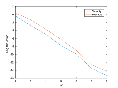
6.2 Ex-2 : Stokes equations with boundary condition (B15)

Let $\Omega=[0,1]^{2}$ . Let $\Gamma_{0}=\left\{(0,x_{2})\mathrel{\mathop{\mathchar 58\relax}}0\leq x_{2}\leq 1\right\}\cup\left\{(x_{1},1)\mathrel{\mathop{\mathchar 58\relax}}0\leq x_{1}\leq 1\right\}\cup\left\{(1,x_{2})\mathrel{\mathop{\mathchar 58\relax}}0\leq x_{2}\leq 1\right\}$ and $\Gamma_{1}=\left\{(x_{1},0)\mathrel{\mathop{\mathchar 58\relax}}0\leq x_{1}\leq 1\right\}$ . We have chosen the data with a set of the exact solutions [37]

\displaystyle\begin{cases}u_{1}=sin(\pi x_{1})sin(\pi x_{2}),\\ u_{2}=sin(\pi x_{1})sin(\pi x_{2}),\\ p=cos(\pi x_{1})exp(x_{1}x_{2}),\end{cases}

with boundary conditions $\mbox{\boldmath$u$}=0\quad\!\!\!\mbox{on}\quad\!\!\!\Gamma_{0}$ and $\mbox{\boldmath$u$}_{\mbox{\boldmath$n$}}=0,\sigma_{\mbox{\boldmath$\tau$}}=\omega_{\mbox{\boldmath$\tau$}}\quad\!\!\!\mbox{on}\quad\!\!\!\Gamma_{1}$ (B15). Table 3 shows the errors $\|E_{\mathbf{u}}\|_{1}$ , $\|E_{p}\|_{0}$ and $\|E_{c}\|_{0}$ and the number of iterations for various values of $W$ . The exact solution is non-algebraic in nature and we can see that the number of iterations is high compared to the number of iterations in example 1.

$W$	${\\|E_{\mbox{\boldmath$u$}}\\|}_{1}$	$\\|{E_{p}}\\|_{0}$	$\\|E_{c}\\|_{0}$	itr
2	7.0505E-01	1.5337E+00	4.0524E-01	15
3	1.0688E-01	1.0022E+00	6.2620E-02	91
4	6.8930E-03	2.4056E-02	2.202E+00	270
5	4.0976E-04	1.9562E-03	3.9979E-04	372
6	4.9890E-05	1.2332E-04	3.1869E-05	425
7	1.3691E-06	3.4167E-06	1.4384E-06	564
8	2.1645E-07	6.5360E-07	1.1044E-07	637

Table 3:

\|E_{\mbox{\boldmath$u$}}\|_{1}

\|E_{p}\|_{0}

and

\|E_{c}\|_{0}

for various values of

W

for Ex-2

Figure 1 presents the log of the errors $\|E_{\mathbf{u}}\|_{1}$ , $\|E_{p}\|_{0}$ against $W$ . The graph is almost linear and this confirms the exponetial accuracy of the numerical method.

Refer to caption — Figure 1: Log of errors $\|E_{\mathbf{u}}\|_{1}$ , $\|E_{p}\|_{0}$ against $W$ for Ex-2

6.3 Ex-3: Stokes equations with boundary condition (B5)

Consider Stokes equations with boundary conditions $p=0,\mbox{\boldmath$n$}\times\mbox{\boldmath$u$}=0$ (B5) with zero right hand side, on boundary of $\Omega=\left\{(-1,1)\times(-1,1)\right\}\setminus\left\{(0,1)\times(-1,0)\right\}$ such that

\displaystyle\begin{cases}u_{1}=-x_{2}(x_{2}^{2}-1),\\ u_{2}=-x_{1}({x_{1}}^{2}-1),\\ p=x_{1}x_{2}({x_{1}}^{2}-1)({x_{2}}^{2}-1),\end{cases}

form a set of the exact solutions [32]. Table 4 shows the errors $\|E_{\mathbf{u}}\|_{1}$ , $\|E_{p}\|_{0}$ and $\|E_{c}\|_{0}$ and the number of iterations for various values of $W$ . The numerical results confirm the fast convergence of the numerical scheme.

$W$	$\\|E_{\mbox{\boldmath$u$}}\\|_{1}$	$\\|E_{p}\\|_{0}$	$\\|E_{c}\\|_{0}$	itr
2	1.2903E-01	9.5655E-02	1.1322E-01	24
3	1.3147E-03	5.8071E-04	3.9079E-04	32
4	7.0454E-04	5.2770E-05	2.9696E-05	48
5	1.9117E-05	1.7295E-05	5.1751E-06	69
6	1.2540E-07	4.7325E-08	4.0931E-08	97

Table 4:

\|E_{\mbox{\boldmath$u$}}\|_{1}

\|E_{p}\|_{0}

and

\|E_{c}\|_{0}

for various values of

W

for Ex-3

6.4 Ex-4: Stokes equations with boundary condition (B12)

We consider Stokes equations on $\Omega=[-1,1]^{2}$ ,

\displaystyle\begin{cases}\Gamma_{1}=\left\{(x_{1},x_{2})\mathrel{\mathop{\mathchar 58\relax}}-1<x_{1}<1,x_{2}=\pm 1\right\},\\ \Gamma_{2}=\left\{(x_{1},x_{2})\mathrel{\mathop{\mathchar 58\relax}}x_{1}=-1,-1<x_{2}<1\right\},\\ \Gamma_{3}=\left\{(x_{1},x_{2})\mathrel{\mathop{\mathchar 58\relax}}x_{1}=1,-1<x_{2}<1\right\}.\end{cases}

Force function and boundary data are chosen such that

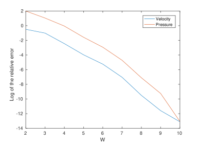
\displaystyle\begin{cases}u_{1}=sin\pi x_{1}sin\pi x_{2}\\ u_{2}=cos\pi x_{1}cos\pi x_{2}\\ p=x_{1}x_{2}\end{cases}

form a set of the exact solutions to the Stokes equations with boundary condition (B12). The given domain is divided into four elements with uniform step sizes one in each direction. The approximate solution is obtained and Table 5 shows the relative errors $\frac{\|E_{\mathbf{u}}\|_{1}}{\left\|\mathbf{u}\right\|_{1}}$ , $\frac{\|E_{p}\|_{0}}{\left\|p\right\|_{0}}$ and $\|E_{c}\|_{0}$ and the number of iterations for various values of $W$ . The number of iterations is high because of the non-algebraic nature of the exact solution and also the pressure and mixed conditions on the boundary.

$W$	$\frac{\\|E_{\mathbf{u}}\\|_{1}}{\left\\|\mathbf{u}\right\\|_{1}}$	$\frac{\\|E_{p}\\|_{0}}{\left\\|p\right\\|_{0}}$	$\\|E_{c}\\|_{0}$	itr
2	6.0646E-01	7.3160E+00	5.3414E+00	11
3	3.6217E-01	2.8203E+00	1.8667E+00	24
4	8.6433E-02	9.4839E-01	5.2985E-01	40
5	1.8758E-02	2.0515E-01	1.0918E-01	116
6	5.2405E-03	5.2657E-02	2.4415E-02	200
7	8.7689E-04	8.9130E-03	4.4200E-03	356
8	7.4496E-05	8.2511E-04	4.0602E-04	722
9	9.3018E-06	9.6641E-05	4.9851E-05	1153
10	2.0333E-06	2.1330E-05	1.1979E-05	1675

Table 5:

\frac{\|E_{\mathbf{u}}\|_{1}}{\left\|\mathbf{u}\right\|_{1}}

\frac{\|E_{p}\|_{0}}{\left\|p\right\|_{0}}

and

\|E_{c}\|_{0}

for various values of

W

for Ex-4

Figure 2 shows the log of the relative errors $\frac{\|E_{\mathbf{u}}\|_{1}}{\left\|\mathbf{u}\right\|_{1}},\frac{\|E_{p}\|_{0}}{\left\|p\right\|_{0}}$ against $W$ . The graph is almost linear and this shows that method is exponentially accurate.

6.5 Ex-5: Stokes equations with boundary conditions (B7) on $[-1,1]^{2}$

Here we consider Stokes equations with the following boundary conditions on $[-1,1]^{2}$ :

\displaystyle\begin{cases}\mathbf{u.n}=g,[(2\mathbb{D}\mathbf{u})\mathbf{n}]_{\mbox{\boldmath$\tau$}}=\mbox{\boldmath$h$}\,\,\textrm{on}\,\,\{(x_{1},x_{2})\mathrel{\mathop{\mathchar 58\relax}}-1<x_{1}<1,x_{2}=1\}\\ \mathbf{u=g_{1}}\,\textrm{\,on\,\,the\,\,other\,\,sides\,\,of}\,\,[-1,1]^{2}.\end{cases}

Data is chosen such that the exact solution of the boundary value problem is

\displaystyle\begin{cases}u_{1}=sin\,\pi x_{1}\,sin\,\pi x_{2},\\ u_{2}=cos\,\pi x_{1}\,cos\,\pi x_{2}\\ p=x_{1}x_{2\,\,\,\,\,\,\,\,\,\,\,\,\,\,\,\,\,\,\,}.\end{cases}

The given domain is divided into four square elements with equal sides of length one. The error in the approximate solution is obtained for different values of $W.$ Table 6 shows the relative errors $\frac{\left\|E_{\mathbf{u}}\right\|_{1}}{\left\|\mathbf{u}\right\|_{1}},\frac{\left\|E_{p}\right\|_{0}}{\left\|p\right\|_{0}}$ and $\left\|E_{c}\right\|_{0}$ for different values of $W.$ The decay of the error $\|E_{c}\|_{0}$ shows the mass conserving property of the numerical scheme.

$W$	$\frac{\left\\|E_{\mathbf{u}}\right\\|_{1}}{\left\\|\mathbf{u}\right\\|_{1}}$	$\frac{\left\\|E_{p}\right\\|_{0}}{\left\\|p\right\\|_{0}}$	$\left\\|E_{c}\right\\|_{0}$	itr
2	7.5989E-01	2.9508E+00	5.7610E+00	19
4	6.1126E-02	4.2430E-01	3.6661E-01	176
6	1.7586E-03	1.2257E-02	1.1238E-02	421
8	7.2036E-05	5.7808E-04	3.6999E-04	734
10	1.9453E-06	9.8102E-05	9.6509E-06	1693

Table 6:

\frac{\left\|E_{\mathbf{u}}\right\|_{1}}{\left\|\mathbf{u}\right\|_{1}},\frac{\left\|E_{p}\right\|_{0}}{\left\|p\right\|_{0}}

and

\left\|E_{c}\right\|_{0}

for different values of

W

for Ex-5

6.6 Ex-6: Stokes equations with boundary conditions (B3) on $[0,1]^{2}$

Here we consider Stokes equations with the following boundary conditions on $[0,1]^{2}$

\displaystyle\begin{cases}\mathbf{u.n}=g,[(\nabla\mathbf{u}+(\nabla\mathbf{u})^{T}-pI)\mathbf{n}+\mathbf{u}]_{\mathbf{\mbox{\boldmath$\tau$}}}=\mathbf{h}\,\,\textrm{on}\,\,\{(x_{1},x_{2})\mathrel{\mathop{\mathchar 58\relax}}0<x_{1}<1,x_{2}=0\}\\ \mathbf{u=g_{1}}\,\textrm{\,on\,\,the\,\,other\,\,sides\,\,of}\,\,[0,1]^{2}.\end{cases}

Data is chosen such that the exact solution of the boundary value problem is

\displaystyle\begin{cases}u_{1}=sin\,\pi x_{1}\,sin\,\pi x_{2},\\ u_{2}=cos\,\pi x_{1}\,cos\,\pi x_{2},\\ p=x_{1}x_{2}.\end{cases}

The given domain is divided into four square elements with equal side length $h=0.5.$ The error in the approximate solution is obtained for different values of $W.$ Table 7 shows the relative errors $\frac{\left\|E_{\mathbf{u}}\right\|_{1}}{\left\|\mathbf{u}\right\|_{1}},\frac{\left\|E_{p}\right\|_{0}}{\left\|p\right\|_{0}}$ and $\left\|E_{c}\right\|_{0}$ for different values of $W.$

$W$	$\frac{\left\\|E_{\mathbf{u}}\right\\|_{1}}{\left\\|\mathbf{u}\right\\|_{1}}$	$\frac{\left\\|E_{p}\right\\|_{0}}{\left\\|p\right\\|_{0}}$	$\left\\|E_{c}\right\\|_{0}$	itr
2	1.6561E-01	2.4997E+00	4.7065E-01	10
4	1.0226E-02	1.1310E-01	2.6468E-02	107
6	7.2611E-04	8.7936E-03	1.9605E-03	419
8	5.3046E-05	6.2276E-04	1.6031E-04	1091

Table 7:

\frac{\left\|E_{\mathbf{u}}\right\|_{1}}{\left\|\mathbf{u}\right\|_{1}},\frac{\left\|E_{p}\right\|_{0}}{\left\|p\right\|_{0}}

and

\left\|E_{c}\right\|_{0}

for different values of

W.

6.7 Ex-7: Stokes equations with boundary conditions (B10) on $[0,1]^{2}$

Here we consider Stokes equations with the following boundary conditions on $[0,1]^{2}$

\displaystyle\begin{cases}\mathbf{u_{\mbox{\boldmath$\tau$}}}=0,[(\nabla\mathbf{u}-pI)\mathbf{n}].\textrm{$\mathbf{n}$}=\mathbf{g}\,\,\textrm{on}\,\,\{(x_{1},x_{2})\mathrel{\mathop{\mathchar 58\relax}}0<x_{1}<1,x_{2}=0\}\\ \mathbf{u=g_{1}}\,\textrm{\,on\,\,the\,\,other\,\,sides\,\,of}\,\,[0,1]^{2}.\end{cases}

Data is chosen such that the exact solution of the boundary value problem is

\displaystyle\begin{cases}u_{1}=sin\,\pi x_{1}\,sin\,\pi x_{2},\\ u_{2}=cos\,\pi x_{1}\,cos\,\pi x_{2},\\ p=x_{1}x_{2}.\end{cases}

The given domain is divided into four square elements with equal side lengths $h=0.5.$ The error in the approximate solution is obtained for different values of $W.$ Table 8 shows the relative errors $\frac{\left\|E_{\mathbf{u}}\right\|_{1}}{\left\|\mathbf{u}\right\|_{1}},\frac{\left\|E_{p}\right\|_{0}}{\left\|p\right\|_{0}}$ and $\left\|E_{c}\right\|_{0}$ for different values of $W.$ The decay of the errors confirm the exponential decay of the numerical method. The decay of the error confirms the exponential accuracy of the numerical method.

$W$	$\frac{\left\\|E_{\mathbf{u}}\right\\|_{1}}{\left\\|\mathbf{u}\right\\|_{1}}$	$\frac{\left\\|E_{p}\right\\|_{0}}{\left\\|p\right\\|_{0}}$	$\left\\|E_{c}\right\\|_{0}$	itr
2	1.7125E-01	1.9638E+00	5.2266E+00	9
4	1.1853E-02	1.6104E-01	2.8415E-02	106
6	5.7420E-04	7.0487E-03	1.6417E-03	402
8	4.4148E-05	5.2272E-04	1.2899E04	1039

Table 8:

\frac{\left\|E_{\mathbf{u}}\right\|_{1}}{\left\|\mathbf{u}\right\|_{1}},\frac{\left\|E_{p}\right\|_{0}}{\left\|p\right\|_{0}}

and

\left\|E_{c}\right\|_{0}

for different values of

W.

6.8 Ex-8: Stokes equations with boundary condition (B5) on $[-1,1]^{3}$

Here we consider Stokes equations with boundary conditions $\mbox{\boldmath$u$}\times\mbox{\boldmath$n$}=\mbox{\boldmath$g$}\times\mbox{\boldmath$n$},p=\phi$ on $\Omega=[-1,1]^{3}$ . The data are chosen such that

	$\displaystyle u_{1}(x_{1},x_{2},x_{3})=4x_{1}^{2}x_{2}x_{3}(1-x_{1})^{2}(1-x_{2})(1-x_{3})(x_{3}-x_{2}),$
	$\displaystyle u_{2}(x_{1},x_{2},x_{3})=4x_{1}x_{2}^{2}x_{2}x_{3}(1-x_{1})(1-x_{2})^{2}(1-x_{3})(x_{1}-x_{3}),$
	$\displaystyle u_{3}(x_{1},x_{2},x_{3})=4x_{1}x_{2}x_{3}^{2}(1-x_{1})(1-x_{2})(1-x_{3})^{2}(x_{2}-x_{1}),$
	$\displaystyle p(x_{1},x_{2},x_{3})=-2x_{1}x_{2}x_{3}+x_{1}^{2}+x_{2}^{2}+x_{3}^{2}+x_{1}x_{2}+x_{1}x_{3}+x_{2}x_{3}$
	$\displaystyle\quad\quad\quad\quad\quad\quad\quad-x_{1}-x_{2}-x_{3},$

form an exact solution to Stokes problem with boundary condition (B5). Here we consider a single element i.e $[-1,1]^{3}$ . Table 9 shows the errors $\|E_{\mathbf{u}}\|_{1}$ , $\|E_{p}\|_{0}$ and $\|E_{c}\|_{0}$ and the number of iterations for various values of $W$ .

$W$	${\\|E_{\mbox{\boldmath$u$}}\\|}_{1}$	${\\|E_{p}\\|}_{0}$	${\\|E_{c}\\|}_{0}$	itr
2	1.1089E+01	3.6122E-01	2.5517E+00	21
4	8.2164E-03	5.7646E-03	3.6079E-03	91
6	2.3867E-04	1.1298E-04	6.6529E-05	432
8	4.5072E-05	2.1736E-05	1.1137E-05	1512

Table 9:

\|E_{\mbox{\boldmath$u$}}\|_{1}

\|E_{p}\|_{0}

and

\|E_{c}\|_{0}

for various values of

W

for Ex-8

7 Conclusion and future work

Here we have proposed a unified approach for Stokes equations with various non-standard boundary conditions based on a non-conforming least-squares spectral element method. A minimal amount of change, only related to the boundary terms is required in the implementation part with the change of boundary conditions. Exponential accuracy has been observed with various boundary conditions in different test cases. For some cases, we have plotted the logarithm of error versus degree of the polynomial, which comes out to be almost straight line, which graphically ensures exponential accuracy. For some of the test problems, iteration count is high which is due to the complexity in approximating non-algebraic solutions and also boundary conditions involving derivatives. We have presented numerical results for seven different types of boundary conditions. One can see similar results in other cases.

We expect similar behaviour for Navier-Stokes equations with these non-standard boundary conditions to yield similar order accuracy, which is an ongoing investigation.

Declaration

Authors declare that they do not have any conflict of interest.

References

[1] H. Abboud, F.E. Chami and T. Sayah, A priori and a posteriori estimates for three dimensional Stokes equations with non-standard boundary conditions, Numer. Methods Partial Differ. Equ., 28(4), 1178-1193, 2012.
[2] H. Abboud, F.E. Chami and T. Sayah, Error estimates for three-dimensional Stokes problem with non-standard boundary conditions, C.R. Acad. Sci. Paris, 349, 523-528, 2011.
[3] P. Acevedo, C. Amrouche, C. Conca and A. Ghosh, Stokes and Navier-Stokes equations with Navier boundary condition, Comptes Rendus Mathematique, 357(2), 115-119, 2019.
[4] S. Agmon, A. Douglis and L. Nirenberg, Estimates near the boundary for solutions of elliptic partial differential equations satisfying general boundary conditions II, Comm. Pure Appl. Math. 17, 35-92, 1964.
[5] M. Amara, E.C. Vera and D. Trujillo, Vorticity-velocity -pressure formulations for Stokes problem, Math. Comput., 73(248), 1673-1697, 2003.
[6] K. Amoura, C. Bernardi, N. Chorfi and S. Saadi, Spectral discretization of the Stokes problem with mixed boundary conditions, Progress in Computational Physics, 20, 42-61, 2012.
[7] C. Amrouche, C. Bernardi, M. Dauge and V. Girault, Vector potentials in three dimensional nonsmooth domains, Math. Methods Appl. Sci., 21, 823-864, 1998.
[8] C. Amrouche and A. Rejaiba, $L^{p}$ theory for Stokes and Navier Stokes equations with Navier boundary condition, J. Diff. Eq., 256, 1515-1547, 2014.
[9] C. Amrouche and N.E.H. Seloula, Stokes equations and elliptic systems with non standard boundary conditions, Comptes Rendus Math., 349 (11-12), 704-708, 2011.
[10] C. Amrouche and N.H. Seloula, On the Stokes equations with Navier-type boundary conditions, Diff. Eq. Appl., 3(4), 581-607, 2011.
[11] C. Amrouche and N.H. Seloula, $L^{p}$ theory for vector potentials and Sobolev inequalities for vector fields : Application to the Stokes equations with pressure boundary conditions, Math. Methods Appl. Sci., 23, 37-92, 2013.
[12] G.R. Barrenechea, M. Basy and V. Dolean, Stabilized hybrid discontinuous Galerkin methods for the Stokes problem with non-standard boundary conditions, Lecture notes in computational engineering, 179-189, 2018.
[13] C. Begue, C. Conca, F. Murat and O. Pironneau, Les Ã©quations de Stokes et de Navier-Stokes avec des conditions aux limites sur la pression, Nonlinear Partial Differential Equations and Their Applications, College de France Seminar, Pitman Res. Notes in Math., 181, 179-264, 1989.
[14] A. Bendali, J.-M. Dominguez and S. Gallic, A Variational Approach for the Vector Potential Formulation of the Stokes and Navier-Stokes Problems in Three Dimensional Domains, J. Math. Anal, and Appl., 107, 537-560, 1985.
[15] J.M. Bernard, Non-standard Stokes and Navier-Stokes problems : existence and regularity in stationary case, Math. Meth. Appl. Sci., 25, 627-661, 2002.
[16] J.M. Bernard, Spectral discretizations of the Stokes equations with non-standard boundary conditions,J Sci Comput., 20(3), 355-377, 2004.
[17] C. Bernardi, C. Canuto and Y. Maday , Spectral approximations of the Stokes equations with boundary conditions on the pressure, SIAM. J. Numer. Anal., 28(2), 333-369, 1991.
[18] C. Bernardi and N. Chorfi, Spectral discretization of the vorticity, velocity and pressure formulation of the Stokes problem, SIAM J. Numer. Anal.,44(2), 826-850, 2006.
[19] C. Bernardi, F. Hecht and F.Z. Nouri, A new finite element discretization of the Stokes problem coupled with Darcy equations, IMA J. Numer. Anal., 30, 61-93, 2010.
[20] C. Bernardi, F. Hecht and O. Pironneau, Coupling Darcy and Stokes equations for porous media with cracks, Math. Model. Nemer. Anal., 39, 7-35, 2005.
[21] S. Bertoluzza, V. Chabannes, C. Prud’homme and M. Szopas, Boundary conditions involving pressure for the Stokes problem and applications in computational hemodynamics, Comput. Methods Appl. Mech. Eng., 322, 58-80, 2017.
[22] P.B. Bochev and M.D. Gunzburger, Finite element methods of least-squares type, SIAM Rev., 40(4), 789-837, 1998.
[23] P.B. Bochev and M.D. Gunzburger, Least-squares methods for the velocity-pressure-stress formulation of the Stokes equations, Comput. Methods Appl. Mech. Engrg , 126, 267-287, 1995.
[24] J.H. Bramble and P. Lee, On variational formulations for the Stokes equations with nonstandard boundary conditions, Math. Model. Numer. Anal., 28(7), 903-919, 1994.
[25] Z. Cai, T.A. Manteuffel and S.F. Mccormick, First -order system least squares for velocity-vorticity-pressure form of the Stokes equations, with application to linear elasticity, Electron. Trans. Numer. Anal., 3, 150-159, 1995.
[26] C.L. Chang and S.Y. Yang, Analysis of the $L^{2}$ least-squares finite element method for the velocity-vorticity-pressure Stokes equations with velocity boundary conditions, Appl. Math. Comput., 130, 121-144, 2002.
[27] C.L. Chang and J. Nelson, Least-squares finite element method for the Stokes problem with zero residual of mass conservation, SIAM J. Numer. Anal., 34, 480-489, 1997.
[28] C. Conca, C. Pares, O. Pironneau and M. Thrift, Navier-Stokes equations with imposed pressure and velocity fluxes, Int. J. Numer. Methods Fluids, 20, 267-287, 1995.
[29] C. Conca, F. Murat and O. Pironneau, The Stokes and Navier-Stokes equations with boundary conditions involving the pressure, Japan J. Math., 20(2), 279-318, 1994.
[30] J.M. Deang and M.D. Gunzburger, Issues related to least-squares finite element methods for the Stokes equations, SIAM J. Sci. Comput., 20, 878-906, 1999.
[31] J.-M. Dominguez, Formulations en Potential Vecteur du systÃšme de Stokes dans un Domaine de $R^{3}$ , Pub. lab. An. Num., L.A., 189, 1983.
[32] S. Du and H. Duan, Analysis of a stabilized finite element method for Stokes equations of velocity boundary condition and pressure boundary condition, J. Comput. Appl. Math., 337(C), 290-318, 2018.
[33] P. K. Dutt, N. Kishore Kumar and C. S. Upadhyay, Nonconforming h-p spectral element methods for elliptic problems, Proc. Indian Acad. Sci (Math. Sci.), 117, 109-145, 2007.
[34] V. Girault, Incompressible Finite Element Methods for Navier-Stokes Ã©quations with Nonstandard Boundary Conditions in $R^{3}$ , Math. Comp., 51, 55- 74, 1988.
[35] K. P. Gostaf and O. Pironneau, Pressure boundary conditions for blood flows, Chin. Ann. Math., Ser. B, 36, 829-842, 2015.
[36] T.R. Hughes, L.P. Franca, A new finite element formulation for computational fluid dynamics : VII. The Stokes problem with various well-posed boundary conditions : symmetric formulations that converge for all velocity/pressure spaces, Comput. methods Appl. Mech., 65, 85-96, 1987.
[37] B.-N. Jiang and C.L. Chang, Least-squares finite elements for Stokes problem, Comput. Methods Appl. Mech, 78, 297-311, 1990.
[38] S.D. Kim, H.C. Lee and B.C. Shin, Least-squares spectral collocation method for the Stokes equations, Numer. Methods Partial Differ. Equ., 20(1), 128-139, 2003.
[39] B.N. Jiang, On the least-squares method, Comput. Methods Appl. Mech. Engrg, 152, 239-257, 1998.
[40] D. Medkova, Several non-standard problems for the stationary Stokes problem, Analysis, 40(1), 1-17, 2020.
[41] D. Medkova, One problem of the Navier type for the Stokes system in planar domains, J. Diff. Equ., 261, 5670-5689, 2016.
[42] S. Mohapatra, Pravir K. Dutt, B. V. Rathish Kumar and Marc I. Gerritsma, Non-conforming least squares spectral element method for Stokes equations on non-smooth domains, J. of Comp. Appl. Math., 372, 112696, 2020.
[43] S. Mohapatra and A. Husain, Least-squares spectral element method for three dimensional Stokes equations, Applied Numer. Math., 102, 31-54, 2016.
[44] S. Mohapatra and S. Ganesan, Non-Conforming least squares spectral element formulation for Oseen Equations with applications to Navier-Stokes equations, Num. Fun. Ana. and Opti., 37(10), 1295-1311, 2016.
[45] M.A. Ol’shanskii, On the Stokes problem with model boundary conditions, Mat. Sb., 188(4), 603-620, 1997.
[46] Y. Ohhara, M. Oshima, T. Iwai, H. Kitajima, Y. Yajima, K. Mitsudo, A. Krdy, and I. Tohnai, Investigation of blood flow in the external carotid artery and its branches with a new 0D peripheral model, BioMed. Eng. OnLine, 15:16, 2016.
[47] M.M.J Proot and M.I. Gerritsma, A least-squares spectral element formulation for the Stokes problem, J. Sci. Comput., 17, 285-296, 2002.
[48] M. Proot and M.I. Gerritsma, Least-squares spectral elements applied to the Stokes problem, J. Comput. Phys., 181, 454-477, 2002.
[49] M.M.J Proot and M.I. Gerritsma, Mass and momentum conservation of the least-squares spectral element method for Stokes problem, J. Sci. Comput., 27, 389-401, 2006.
[50] A. Russo and A. Tartaglione, On the Navier problem for the stationary Navier-Stokes equations, J. Diff. Eq., 251, 2387-2408, 2011.
[51] Ch. Schwab, $p$ and $h-p$ Finite element methods, Clarendon Press, Oxford, 1998.
[52] N. Saito, On the Stokes equations with the leak and slip boundary conditions of friction type : regularity of solutions, Publ. RIMS, Kyoto Univ., 40, 345-383, 2004.
[53] S. Saito and L.E. Scriven, Study of coating flow by the finite element method, J. Comp. Phys., 42, 53-76, 1981.
[54] J. Silliman and L.E. Scriven, Separating flow near a static contact line : slip at a wallsand shape of a free surface,J. Comp. Phys., 34, 287-313, 1980.
[55] P.A. Tapia, C. Amrouche, C. Conca and A. Ghosh, Stokes and Navier-Stokes equations with Navier boundary conditions, J Diff. Equ. , 285, 258-320, 2021.
[56] S.K. Tomar, h-p Spectral element methods for elliptic problems on non-smooth domains using parallel computers, Ph.D. thesis (India: IIT Kanpur) (2001); Reprint available as Tec. Rep. no. 1631, Department of Applied Mathematics, University of Twente, The Netherlands. http://www.math.utwente.nl/publications.
[57] Y. Tokuda, M.-H. Song, Y. Ueda, A. Usui, T. Akita, S. Yoneyama and S. Maruyama, Three dimensional numerical simulation of blood flow in the aortic arch during cardiopulmnary bypass, Eur. J. Cardiothorac. Surg., 33, 164-167, 2008.
[58] R. Verfurth, Finite element approximation on incompressible Navier-Stokes equations with slip boundary condition, Numerische Mathematik, 50, 697-721, 1986.
[59] R. Verfurth, Mixed Finite Element Approximation of the Vector Potential, Numer. Math., 50, 685-695, 1987.
[60] H.B.D. Viega, Regularity for Stokes and generalized Stokes systems under nonhomogeneous slip-type boundary conditions, Adv. Diff. Equ., 9 (9-10), 1079-1114, 2004.
[61] I. E. Vignon-Clementel, C. A. Figueroa, K. E. Jansen and C. A. Taylor, Outflow boundary conditions for three dimensional finite element modeling of blood flow and pressure arteries, Comput. Methods Appl. Mech. Engrg., 195, 3776-3796, 2006.
[62] I. E. Vignon-Clementel, C. A. Figueroa, K. E. Jansen and C. A. Taylor, Outflow boundary conditions for 3D simulations of non-periodic blood flow and pressure fields in deformable arteries. Comput. Methods Biomech. Biomed. Engin., 13, 625-640, 2010.

	$\displaystyle\mathcal{V}^{L,W}(\mbox{\boldmath$u$},p)$	$\displaystyle=\sum_{l=1}^{L}\\|\mathcal{L}(\mbox{\boldmath$u$}_{l},p_{l})\\|_{0,Q}^{2}+\sum_{l=1}^{L}\\|\mathcal{D}\mbox{\boldmath$u$}_{l}\\|_{1,Q}^{2}$
		$\displaystyle+\sum_{\Gamma_{l,i}\subseteq\bar{\Omega}\setminus\Gamma}\left(\\|[\mbox{\boldmath$u$}]\\|_{0,\Gamma_{l,i}}^{2}+\sum_{k=1}^{n}\\|[\mbox{\boldmath$u$}_{x_{k}}]\\|_{\frac{1}{2},\Gamma_{l,i}}^{2}+\\|[p]\\|_{\frac{1}{2},\Gamma_{l,i}}^{2}\right)$
		$\displaystyle+\sum_{\Gamma_{l,i}\subset\Gamma}\\|\mbox{\boldmath$u$}_{l}\cdot\mbox{\boldmath$n$}\\|_{\frac{3}{2},\Gamma_{l,i}}^{2}+\sum_{\Gamma_{l,i}\subset\Gamma}\\|(\nabla\times\mbox{\boldmath$u$}_{l})\times\mbox{\boldmath$n$}\\|_{\frac{1}{2},\Gamma_{l,i}}^{2}.$

	$\displaystyle{\\|\mbox{\boldmath$u$}\cdot\mbox{\boldmath$n$}\\|}_{\mbox{\boldmath$H$}^{\frac{3}{2}}(\Gamma)}^{2}+{\\|\nabla\times\mbox{\boldmath$u$}\times\mbox{\boldmath$n$}\\|}_{\mbox{\boldmath$H$}^{\frac{1}{2}}(\Gamma)}^{2}$
	$\displaystyle\leq c\bigg{(}\left\\|\mbox{\boldmath$u$}\right\\|_{\mbox{\boldmath$H$}^{\frac{3}{2}}(\Gamma)}^{2}+\\|\frac{\partial\mbox{\boldmath$u$}}{\partial\mbox{\boldmath$n$}}\\|_{\mbox{\boldmath$H$}^{\frac{1}{2}}(\Gamma)}\bigg{)}$
	$\displaystyle\leq c(\ln W)^{2}\left(\sum_{\Gamma_{l,i}\subseteq\bar{\Omega}\setminus\Gamma}\left(\left\\|[\mbox{\boldmath$u$}]\right\\|_{{}_{0,\Gamma_{l,i}}}^{2}+\sum_{k=1}^{n}\left\\|[\mbox{\boldmath$u$}_{x_{k}}]\right\\|_{{}_{1/2,\Gamma_{l,i}}}^{2}\right)+\sum_{\Gamma_{l,i}\subset\Gamma}\left\\|\mbox{\boldmath$u$}\right\\|_{{}_{\frac{3}{2},\Gamma_{l,i}}}^{2}\right).$
	(Using estimates and techniques from [33], [42])

	$\displaystyle\mathcal{V}^{L,W}(\mbox{\boldmath$u$},p)$	$\displaystyle=\sum_{l=1}^{L}\\|\mathcal{L}(\mbox{\boldmath$u$}_{l},p_{l})\\|_{0,Q}^{2}+\sum_{l=1}^{L}\\|\mathcal{D}\mbox{\boldmath$u$}_{l}\\|_{1,Q}^{2}$
		$\displaystyle+\sum_{\Gamma_{l,i}\subseteq\bar{\Omega}\setminus\Gamma}\left(\\|[\mbox{\boldmath$u$}]\\|_{0,\Gamma_{l,i}}^{2}+\sum_{k=1}^{n}\\|[\mbox{\boldmath$u$}_{x_{k}}]\\|_{\frac{1}{2},\Gamma_{l,i}}^{2}+\\|[p]\\|_{\frac{1}{2},\Gamma_{l,i}}^{2}\right)$
		$\displaystyle+\sum_{\Gamma_{l,i}\subset\Gamma}\\|\mbox{\boldmath$u$}_{l}\times\mbox{\boldmath$n$}\\|_{\frac{3}{2},\Gamma_{l,i}}^{2}+\sum_{\Gamma_{l,i}\subset\Gamma}\\|p_{l}\\|_{\frac{1}{2},\Gamma_{l,i}}^{2}$

	$\displaystyle{\\|\mbox{\boldmath$u$}\times\mbox{\boldmath$n$}\\|}_{\mbox{\boldmath$H$}^{\frac{3}{2}}(\Gamma)}^{2}+{\\|p\\|}_{H^{\frac{1}{2}}(\Gamma)}^{2}$
	$\displaystyle\leq\left\\|\mbox{\boldmath$u$}\right\\|_{\mbox{\boldmath$H$}^{\frac{3}{2}}(\Gamma)}^{2}+\left\\|p\right\\|_{H^{\frac{1}{2}}(\Gamma)}^{2}$
	$\displaystyle\leq c(\ln W)^{2}\left(\sum_{\Gamma_{l,i}\subseteq\bar{\Omega}\setminus\Gamma}\left(\left\\|[\mbox{\boldmath$u$}]\right\\|_{{}_{0,\Gamma_{l,i}}}^{2}+\sum_{k=1}^{n}\left\\|[\mbox{\boldmath$u$}_{x_{k}}]\right\\|_{{}_{1/2,\Gamma_{l,i}}}^{2}\right)+\sum_{\Gamma_{l,i}\subset\Gamma}\left\\|\mbox{\boldmath$u$}\right\\|_{{}_{\frac{3}{2},\Gamma_{l,i}}}^{2}+\left\\|p\right\\|_{{}_{\frac{1}{2},\Gamma_{l,i}}}^{2}\right).$
	(Using estimates and techniques from [33], [42])

	$\displaystyle{\mathcal{R}1}^{L,W}(\mbox{\boldmath$u$},p)$	$\displaystyle=\underbrace{\sum_{l=1}^{L}\\|\mathcal{L}(\mbox{\boldmath$u$}_{l},p_{l})-\mbox{\boldmath$F$}_{l}\\|_{0,\Omega_{l}}^{2}}_{(a)}$
		$\displaystyle+\underbrace{\sum_{l=1}^{L}\\|\mathcal{D}\mbox{\boldmath$u$}_{l}-\chi_{l}\\|_{1,\Omega_{l}}^{2}}_{(b)}$
		$\displaystyle+\underbrace{\sum_{\Gamma_{l}\subset\bar{\Omega}\setminus\Gamma}\left(\\|[\mbox{\boldmath$u$}]\\|_{0,\Gamma_{l}}^{2}+\sum_{k=1}^{n}\\|[\mbox{\boldmath$u$}_{x_{k}}]\\|_{\frac{1}{2},\Gamma_{l}}^{2}+\\|[p]\\|_{\frac{1}{2},\Gamma_{l}}^{2}\right)}_{(c)}$

Least-squares formulations for Stokes equations with non-standard boundary conditions - A unified approach

Abstract

1 Introduction

2 Notations

Remark 2.1.

2.1 Motivations and physical applications

2.2 Theoretical developments on Stokes equations with non-standard boundary conditions

2.3 Computational developments on Stokes equations with non-standard boundary conditions

Remark 2.2.

2.4 Regularity for (𝒖,p)(\mbox{\boldmath$u$},p) in Stokes equations with various non-stanadard boundary conditions

Remark 2.3.

3 Stability estimates

3.1 Stability estimate for Stokes equations with boundary condition (B4)

Theorem 3.1.

Proof.

3.1.1 Stability estimate for Stokes equations with boundary condition (B5)

Theorem 3.2.

Proof.

4 Numerical scheme

Remark 4.1.

Remark 4.2.

5 Error estimates

Theorem 5.1.

Remark 5.1.

6 Numerical results

6.1 Ex-1 : Stokes equations with boundary condition (B14)

6.2 Ex-2 : Stokes equations with boundary condition (B15)

6.3 Ex-3: Stokes equations with boundary condition (B5)

6.4 Ex-4: Stokes equations with boundary condition (B12)

6.5 Ex-5: Stokes equations with boundary conditions (B7) on [−1,1]2[-1,1]^{2}

6.6 Ex-6: Stokes equations with boundary conditions (B3) on [0,1]2[0,1]^{2}

6.7 Ex-7: Stokes equations with boundary conditions (B10) on [0,1]2[0,1]^{2}

6.8 Ex-8: Stokes equations with boundary condition (B5) on [−1,1]3[-1,1]^{3}

7 Conclusion and future work

Declaration

References

2.4 Regularity for $(\mbox{\boldmath$u$},p)$ in Stokes equations with various non-stanadard boundary conditions

6.5 Ex-5: Stokes equations with boundary conditions (B7) on $[-1,1]^{2}$

6.6 Ex-6: Stokes equations with boundary conditions (B3) on $[0,1]^{2}$

6.7 Ex-7: Stokes equations with boundary conditions (B10) on $[0,1]^{2}$

6.8 Ex-8: Stokes equations with boundary condition (B5) on $[-1,1]^{3}$